TSGCNet: Discriminative Geometric Feature Learning with Two-Stream Graph Convolutional Network for 3D Dental Model Segmentation
Abstract
The ability to segment teeth precisely from digitized 3D dental models is an essential task in computer-aided orthodontic surgical planning. To date, deep learning based methods have been popularly used to handle this task. State-of-the-art methods directly concatenate the raw attributes of 3D inputs, namely coordinates and normal vectors of mesh cells, to train a single-stream network for fully-automated tooth segmentation. This, however, has the drawback of ignoring the different geometric meanings provided by those raw attributes. This issue might possibly confuse the network in learning discriminative geometric features and result in many isolated false predictions on the dental model. Against this issue, we propose a two-stream graph convolutional network (TSGCNet) to learn multi-view geometric information from different geometric attributes. Our TSGCNet adopts two graph-learning streams, designed in an input-aware fashion, to extract more discriminative high-level geometric representations from coordinates and normal vectors, respectively. These feature representations learned from the designed two different streams are further fused to integrate the multi-view complementary information for the cell-wise dense prediction task. We evaluate our proposed TSGCNet on a real-patient dataset of dental models acquired by 3D intraoral scanners, and experimental results demonstrate that our method significantly outperforms state-of-the-art methods for 3D shape segmentation.
1 Introduction
An essential task in computer-aided-design system for orthodontic treatment is to provide accurate segmentation of teeth on digitalized 3D dental models reconstructed by intraoral scanners (IOS). This segmentation information can be used for aiding clinical diagnose, providing digital teeth shape information for personal surgical-orthodontic planning, quantifying the difference between expected and clinical treatment results to adjust orthodontic treatment plan, etc. However, segmenting each tooth from the gingiva is practically challenging, mainly due to heterogeneous tooth appearance: i) Although most human teeth have common geometric characteristics, their shapes are unique and vary dramatically across individuals. ii) Orthodontic patients usually have atypical conditions such as missing, crowded and/or misaligned teeth, all of which may produce indistinct tooth boundaries. iii) Noise and occlusion during scanning may result in a partially reconstructed dental surface with missing parts.
To deal with these challenges, various (semi-) automated methods have been proposed for tooth segmentation on 3D dental models. Conventional approaches typically perform segmentation by using pre-selected geometric properties (e.g., the 3D coordinates, normal vectors and curvature) T1; T2; T3; T4; T5; T6; T7; T8 or projecting 3D meshes onto 2D images T9; T10. Due to the requirement of manual initialization, the efficacy of such semi-automated methods relies on the professional knowledge and experience. Furthermore, the robustness of these conventional methods may be hampered since the exclusive use of low-level geometric properties would not be able to segment teeth with extreme appearances accurately.
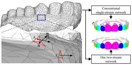
Recently, deep learning-based methods have been proposed to learn task-oriented feature representations for fully-automated tooth segmentation. Some of these methods Dental1; dental2 transformed mesh vertices/cells as ordered 2D image-like (or volumetric) inputs and then applied general convolutional neural networks (CNNs) to perform segmentation. Although straightforward, such operations tend to ignore the unordered nature of geometric data. They also incline to introduce additional computational costs and quantization errors during the potential voxelization stage. To avoid additional data pre-processing, more recent methods dental3; dental4; dental5 applied or extended existing point-cloud segmentation networks to perform vertex/cell-wise semantic labeling of 3D dental meshes. As the network inputs, the 3D coordinates and normal vectors (of mesh vertices/cells) are typically concatenated in these methods to train a single-stream network. However, considering that the coordinate indicates the cell spatial position, while the normal vector represents the cell morphological structure, directly combing these two completely different attributes as a single feature vector tends to weaken their geometric discrimination (e.g., an example is shown in Fig. 1). Hence, this would confuse those conventional single-stream networks in learning discriminative geometric features for cell classification, potentially resulting in isolated false predictions on the dental model.
To resolve these issues, we propose a two-stream graph convolutional network (TSGCNet) in this paper to learn multi-view geometric information for end-to-end tooth segmentation on 3D dental models. In order to eliminate the mutual confusion caused by mixed geometric inputs, our TSGCNet starts with two parallel branches, namely C-stream and N-stream, to learn independently multi-scale feature representations from coordinates and normal vectors, respectively. Besides, considering different geometric meanings of those attributes, the two streams are also constructed by different graph-learning strategies designed in an input-aware fashion. That is, C-stream adopts graph-attention convolutions Att2 to learn the coarse structures of different teeth from coordinates, while the N-stream adopts graph max-pooling to extract distinctive structural details Att2 from the normal vectors, which can further help C-stream to distinguish neighboring cells belonging to different classes (e.g., boundaries between adjacent teeth or between teeth and gingiva). These multi-scale geometric representations produced by the two parallel streams are further fused by the subsequent multi-layer perceptrons (MLPs) to learn complementary multi-view information for dense labeling of all cells on the mesh surface.
The main contributions of this paper can be summarized as follows:
- •
We propose a novel two-stream graph convolutional network that can independently process coordinates and normal vectors to learn more discriminative geometric features for 3D dental model segmentation.
- •
We design two different graph-based feature aggregation modules in an input-aware fashion to consume cell coordinates and normal vectors, respectively. That is, the C-stream adopts graph attention convolutions to capture the coarse structure of teeth from coordinates, while the N-stream extract distinctive structural details from normal vectors.
- •
Our TSGCNet is evaluated on a clinical dataset of 3D dental models for different orthodontic patients digitized by IOS. The experimental results show that our TSGCNet significantly outperform state-of-the-art 3D shape segmentation methods.
2 Related Work
2.1 3D Shape Segmentation
Diverse deep learning methods have been proposed for 3D shape classification and segmentation. Some of these approaches voxelized 3D shapes into regular 3D grids PV1; PV2; PV3; PV4; PV5; PV6; PV7; PV8 or rendered them into multi-view 2D images PM1; PM2; PM3; PM4; PM5, after which standard CNNs were applied to extract features. Such kinds of operations inevitably resulted in spatial information loss and quantization artifacts, inclining to hamper 3D shape segmentation accuracy.
A pioneering network, PointNet Pointnet consisting of successive MLPs and a symmetric function (e.g., global max-pooling), was proposed to learn directly translation-invariant geometric features from irregular 3D data (e.g., point clouds). Although achieving promising results in multiple tasks, PointNet ignored the local spatial relationships on 3D shapes as the architecture learns features for each cell independently. To address this limitation, PointNet++ Pointnet++ constructed a hierarchical architecture with successive sampling layers, grouping layers and PointNet modules. It explicitly captured and integrated local-to-global spatial information on 3D shapes, achieving better performance than the original PointNet in both the classification and segmentation tasks. Similarly, to model spatial dependencies of neighboring points, PointCNN pointcnn adopted an encoder-decoder architecture with -transformations of unordered points to perform general convolutional operations. More recent works further extended PointNet++ by integrating attention modules AM1; AM2, geometry sharing modules geometry and edge branches EdgeBranch. Although those PointNet-like methods can directly consume the raw 3D data for end-to-end inference, they usually missed detailed semantic information since the coarse modeling of local dependencies.
Considering that Graph CNNs have shown great success and flexibility in learning from data with irregular structures, some graph-based methods were also proposed for 3D shape recognition and segmentation. They usually defined the spatial relations between points/cells as a graph and then used spectral-based spectral1; spectral2 or spatial-based spatial1 graph convolutions to aggregate local information. To extract more detailed geometric features, some researchers Att1; Att2; Att3 additionally applied attention mechanism during the feature aggregation step.
2.2 3D Dental Model Segmentation
Conventional tooth segmentation methods using pre-selected geometric properties can be roughly grouped as curvature-based methods T1; T2; T3; T4; T5, contour-line-based methods T6; T7 and harmonic-field-based methods T8. Another commonly used strategy is to project the 3D dental models as 2D images, after which the teeth are segmented in 2D and reprojected back to 3D. Due to the typical requirement of manual steps and domain knowledge, the efficacy of such semi-automated methods heavily depends on the operator experience.
In recent years, several deep learning-based methods have been proposed for fully-automated tooth segmentation on dental models. Typically, Xu et al. dental2 proposed to reshape handcrafted geometric features as 2D image patches to train CNNs for classifying the mesh cells. Tian et al. Dental1 proposed to voxelize the dental model with a sparse octree partitioning PV4, after which 3D CNNs are applied for tooth segmentation. Although those methods using standard CNNs can learn task-oriented feature representations for segmentation, converting the original input into grid format either ignores the unordered nature of the geometric data dental2 or may introduce additional quantization errors during the voxelization step Dental1. To address this limitation, Zanjani et al. dental3 proposed an end-to-end network that integrates PointCNN pointcnn with a discriminator to directly segment the raw dental surfaces acquired by IOS. Lian et al. dental4 extended PointNet Pointnet by adding a multi-scale graph-constrained module to extract fine-grained local geometric features from dental mesh data. Instead of using solely the 3D coordinates (e.g., in dental3), Lian et al. dental4 combined 3D coordinates and normal vectors as the network input to improve the segmentation performance.
However, since coordinates and normal vectors are completely different geometric meanings of a 3D shape, directly combining these low-level features as a single-stream input would confuse the learning of discriminative geometric representations. Different from those methods, our TSGCNet adopts two graph-learning streams, designed in an input-aware, to independently learn feature representations from coordinates and normal vectors. This can eliminate the mutual confusion caused by mixed geometric inputs and extract.
3 The Proposed Method
3.1 Overview
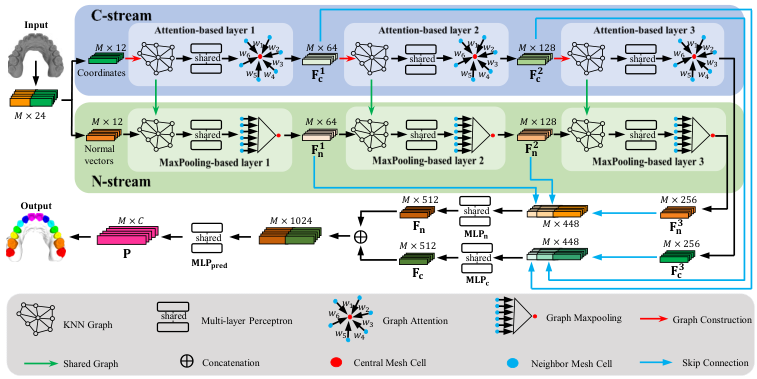
Given a 3D dental model with mesh cells, we define the input of our TSGCNet as a matrix. That is, each specific cell is described by a -dimensional vector, including the 3D coordinates ( elements) and normal vectors ( elements) of four points (i.e., the cell’s three vertices and its central point). As illustrated in Fig. 2, our TSGCNet starts with a two-stream architecture, which adopts a C-stream and a N-stream to learn more discriminative geometric representations from the coordinates and normal vectors, respectively. Thereafter, the features produced by these two complementary streams are further fused to learn higher-level representation for final prediction. The output of our TSGCNet is an matrix, with each row denoting the probabilities of the respective cell belonging to different classes.
3.2 Two-Stream Architecture
C-Stream.
Our C-stream is designed to learn the basic topology of a dental model. As shown in Fig. 2, given the input of a coordinate matrix, a series of graph-attention layers are successively applied in the forward path to extract multi-scale geometric features from the coordinate aspect. In each layer of the C-stream, a KNN graph is first constructed for the cells in terms of the input features. Specifically, for each cell (i.e., a central node), we find its nearest cells with the smallest Euclidean distance in feature space. Let the resulting graph be , where and represent the set of nodes (mesh cells) and the set of edges (defined by KNN connectivity), respectively. For each node , we denote its KNN as .
After building the KNN graph in each layer, a shared MLP is applied to learn embedded features on each . Let (e.g., in the first layer) denote the input feature vector of in the -th layer, and denotes the input feature vector of its -th nearest neighbor . We first calibrate local information for each center, by learning an updated nearest-neighbor representation in terms of and , as:
| (1) |
where indicates the channel-wise concatenation. In this way, the information provided by (encoded in ) can be more consistent with the specific central node , given the fact that could be a nearest neighbor of more than one center, i.e., might be shared by multiple centers.
Additionally, we adopt a graph attention mechanism to aggregate the calibrated neighborhood information to each center. Inspired by Att1; Att2, we choose a learning-based approach to estimate the attention weights for different neighbors. Compared with the strategy of using predefined weights Att3, learning the weights in a task-oriented fashion (e.g., by a lightweight network) can more flexibly capture local geometric characteristics of the dental model for the segmentation task. Specifically, we compute the attention weight of neighbor in the -th layer as:
| (2) |
where the function is implemented as a MLP in this work. It adopts both and as the input, where quantifies the dissimilarity between and while provides detailed neighbor information in the feature space. Finally, the feature aggregation in the -th layer is formulated as:
| (3) |
where indicates the updated feature of center , i.e., the input feature of the (+1)-th layer. In Eq. (3), and are defined by Eq. (2) and Eq. (1), respectively, and performs the element-wise production of two feature vectors.
N-Stream.
Although the C-stream can learn the basic structure of a dental model from the 3D coordinates, it cannot sensitively distinguish between adjacent cells belonging to different classes (e.g., boundaries of teeth). Therefore, as complementary to the C-stream for accurate teeth delineation, we further design a N-stream to extract fine-grained boundary representations from the aspect of normal vectors in local areas.
Our N-stream takes the matrix of normal vectors as input and consists of a series of graph max-pooling layers. Notably, we force each layer in the N-steam to share the same KNN graph with the respective layer in the C-stream. In this way, the graph max-pooling layers can focus on the learning of boundary representations in local regions, thereby avoiding the disturbance of distant cells that have similar normal vectors (but belonging to different classes). For simplicity, we still use the symbols and to denote the input features of a center node and its neighbor , respectively. Similar to the C-stream, the -th layer of the N-stream first uses a MLP to learn the calibrated feature representation for each , i.e., similar to Eq. (1). Thereafter, we apply the channel-wise max-pooling on all neighbors’ calibrated features to produce the boundary representation for the respective center, which can be formulated as:
| (4) |
It is worth mentioning that we use max-pooling (rather than graph attention) in the N-steam since the max operator can sensitively capture the most distinctive features presented at the tooth boundaries.
3.3 Feature Fusion
Considering that the C-stream and the N-stream learn completely different feature representations from two complementary views, fusing their outputs can enable the overall network to comprehensively understand the structure of a dental model. To this end, as shown in Fig. 2, for each stream, we first use skip connections to concatenate its multi-scale cell-wise features from different layers (i.e., or , where denotes the -th layer), yielding a hierarchical feature matrix encoding local-to-global information. A MLP (i.e., MLPc or MLPn) is then applied on this feature matrix to learn higher-level representations (i.e., or ) for the corresponding view (i.e, the C-stream or the N-stream), which can be formulated as follows:
| (5) |
| (6) |
Finally, the feature matrices from two complementary views are concatenated, which is followed by another MLP (i.e., MLPpred) to output an matrix , with each row denoting the probabilities of a specific cell belonging to different classes, which can be formulated as:
| (7) |
We train TSGCNet with cross-entropy segmentation loss, which can be formulated as:
| (8) |
where and denote the predicted and the ground-truth labeling probability for -th class, respectively.
3.4 Implementation Details
Network Details.
As shown in Fig. 2, the TSGCNet architecture consists of a C-stream, a N-stream, and a feature-fusion part. For each branch of the two streams, the MLPs in the first to the third layer contain one 1D Conv with 64 channels, 128 channels, and 256 channels, respectively. The number of each KNN graph is set as 32. We use MLP to implement the graph attention function , which is followed by the channel-wise softmax to normalize the output weights. In the feature fusion part, both MLPc and MLPn contain a 1D Conv with 512 channels, and MLPpred contains four successive 1D Convs, each with 512, 256, 128, and channels, respectively. All 1D Convs are followed by batch normalization and LeakyReLU, except the last one in MLPpred, which is followed by a tensor-reshape operation to output the probability matrix.
Training Details.
Our TSGCNet was trained by minimizing the cross-entropy segmentation loss on two NVIDIA GTX 1080 GPUs for 200 epochs. We use the Adam optimizer with the mini-batch size setting as 4. The initial learning rate was 1e-3, which was reduced by 0.5 decay for every 20 epochs.

| Method | OA | mIoU | T1 | T2 | T3 | T4 | T5 | T6 | T7 | BG |
|---|---|---|---|---|---|---|---|---|---|---|
| PointNetPointnet | 84.95 | 66.86 | 55.31 | 65.31 | 69.35 | 75.47 | 72.21 | 66.18 | 74.71 | 84.86 |
| PointCNNpointcnn | 88.61 | 72.86 | 61.72 | 66.45 | 68.10 | 78.98 | 78.57 | 70.51 | 72.15 | 86.39 |
| PointNet++Pointnet++ | 90.25 | 78.14 | 67.82 | 74.61 | 78.10 | 82.73 | 80.70 | 74.67 | 78.94 | 87.52 |
| DGCNNspatial1 | 91.93 | 84.30 | 82.18 | 79.95 | 82.09 | 87.88 | 86.24 | 80.14 | 84.26 | 91.65 |
| MeshSegNetdental4 | 93.11 | 84.47 | 81.31 | 83.65 | 82.15 | 82.87 | 84.81 | 81.93 | 87.10 | 91.94 |
| Ours | 95.25 | 88.99 | 86.01 | 87.48 | 89.38 | 90.44 | 89.54 | 85.99 | 89.32 | 93.76 |
4 Experimental Results
4.1 Dataset
The studied dataset consists of 80 3D dental models acquired by an IOS for different orthodontic patients. Each raw dental model roughly contains more than 100,000 meshes, which were downsampled to 16,000 (e.g. ) meshes through the reduction of redundant information, while preserving the original topology. The dataset was randomly split as a training set with 64 subjects, and a testing set with 16 subjects. Our target is to automatically segment each dental model as different semantic parts, including the central incisor (T1), lateral incisor (T2), canine/cuspid (T3), 1 premolar (T4), 2 premolar (T5), 1 molar (T6), 2 molar (T7), and background/gingiva (BG). The ground-truth annotations of all dental models were defined by an experienced orthodontist, with a typical example shown in Fig. 3.
4.2 Experimental Setup
Data Augmentation.
We augment the training set by the combination of 1) random translation, and 2) random rotation of each 3D dental model. Specifically, each training dental model is translated with a displacement randomly sampled between and rotated along the -axis with an angle randomly sampled between . In this way, we generate 64 new samples from the original dental models to enrich the diversity of the training set.
Competing Methods.
Our TSGCNet was compared with five state-of-the-art methods for both 3D shape segmentation (i.e., PointNet Pointnet, PointNet++ Pointnet++, PointCNN pointcnn, DGCNN spatial1) and 3D dental model segmentation (i.e., MeshSegNet dental4). All these five competing methods were implemented by their original codes and trained on the same dataset. For the grouping operations of PointNet++ Pointnet++, we deployed the 3D coordinates of the central point of each cell to compute the spatial distance. The overall segmentation performance (averaged over all classes) was quantitatively evaluated by two metrics, i.e., 1) Overall Accuracy (OA), and 2) mean Intersection-over-Union (mIoU). Besides, we also quantify the detailed IoU of each class.
4.3 Comparison with Competing Methods
The overall segmentation results are presented in Table 1. Results show that our method achieves the best performance in terms of both OA and mIoU metrics. In particular, when compared with the competing method in this specific task, MeshSegNet Att2, which directly consumes the combination of coordinates and normal vectors, the proposed TSGCNet still increases the segmentation accuracy by and on the OA and mIoU, respectively. Additionally, our method also significantly outperforms the graph based network DGCNN spatial1, demonstrating the effectiveness of the proposed two-stream mechanism that can learn more discriminative geometric feature representations for accurate tooth segmentation. Furthermore, despite the varying shape appearances of different types of teeth, our method is able to present consistent superior segmentation performance over other approaches by a large margin.
We also visualize the segmentation results (obtained by different methods) for four representative dental models in Fig. 4. In consistency with the quantitative evaluations, we can observe from Fig. 4 that our TSGCNet also qualitatively outperforms all the competing methods, especially for the challenging areas marked by the blue arrows and green dotted circles. Specifically, in the area of teeth misalignment (indicated by the blue arrows in the first two rows), PointNet Pointnet, PointNet++ Pointnet++ and PointCNN pointcnn either result in under-segmentation or over-segmentation. Graph-based competing methods (i.e., DGCNN spatial1 and MeshSegNet dental4) achieve better performance based on the extraction of detailed local spatial information. However, they still fail to capture the complete teeth structure. In contrast, due to the use of complementary information from the C-stream and N-stream, our TSGCNet achieves more accurate results than all the competing methods in these misaligned areas. Besides, from the third and fourth rows of Fig. 4, we can see that our proposed method can also better distinguish the boundaries between adjacent teeth, especially for the two adjacent incisors (indicated by the green dotted circles). Finally, when comparing our method with MeshSegNet dental4 in the fourth row, we can see that MeshSegNet dental4 produces many isolated false predictions on gingiva, even those mislabeled mesh cells are relatively far away from the real tooth area. This further suggests that the direct concatenation of normal vectors and coordinates as a single feature vector (e.g., in MeshSegNet) may confuse the learning of discriminative geometric features in some cases, while the two-stream structure (i.e., in our TSGCNet) is a more appropriate design.

5 Ablation Study
In this section, we conduct detailed ablation studies to evaluate the efficacy of the critical components of our TSGCNet.
5.1 Effectiveness of the Two-Stream Structure
In this series of experiments, we first evaluate the effectiveness of our two-stream structure. Specifically, we remove the N-stream (i.e., only adopting the C-stream with the coordinates as input) or the C-stream (i.e., only adopting the N-stream with the normal vectors as input) to generate two different variants of TSGCNet, which are denoted as TSGCNet-C and TSGCNet-N, respectively. In addition, we also build another single-stream variant of TSCGNet (denoted as TSGCNet-S) that directly learns from the combination of the coordinates and normal vectors. Note that TSGCNet-S has a similar structure to TSGCNet-C but with different input. We compare these three variants with the final TSGCNet, with the quantitative results listed in Table 2. It can been seen that TSGCNet-N and TSGCNet-C led to worse results than both TSGCNet-S and TSGCNet. This justifies the complementarity between the geometric information provided by the coordinates and normal vectors in delineating teeth on dental models. On the other hand, when compared with TSGCNet-S, the original TSGCNet further improves the segmentation accuracy, which suggests the effectiveness of our two-stream structure in extracting the complementary geometric information from the two different views.
| Structure | OA | mIoU |
|---|---|---|
| TSGCNet-C | 83.23 | 63.79 |
| TSGCNet-N | 55.42 | 20.77 |
| TSGCNet-S | 87.25 | 73.44 |
| TSGCNet | 95.25 | 88.99 |
5.2 Effectiveness of Feature-Aggregation Strategy
As described in Section 3.2, we use two different feature aggregation strategies in the C-stream and N-stream of our TSGCNet. Specifically, the graph attention aggregation is used in the C-stream, while the graph max-pooling aggregation in the N-stream. To evaluate the effectiveness of our design, we implement three variants of TSGCNet by changing the feature aggregation strategy in each stream, including 1) both streams use max-pooling, 2) both streams use attention, and 3) C-stream uses max-pooling while N-stream uses attention. For simplicity, we denote those three variants and the original TSGCNet as M+M, A+A, M+A, and A+M, respectively. We then compare the segmentation results of these variants in Table 3. From Table 3, we can see that using attention mechanisms in the C-stream can achieve better performance (please refers to A+M vs. M+M) when compares with the use of max-pooling, which suggests that graph attention aggregation can extract finer details of the tooth shape from coordinates. Besides, using max-pooling in the N-stream can further refine the segmentation results (please refers to A+M vs. A+A). This can be rationally explained by that max-pooling can extract more distinctive morphological features, which in return helps the network to capture difference between neighboring cells, especially at the tooth boundaries.
| Structure | OA | mIoU |
|---|---|---|
| M+M | 94.56 | 86.24 |
| A+A | 95.01 | 87.35 |
| M+A | 93.93 | 85.67 |
| A+M | 95.25 | 88.99 |
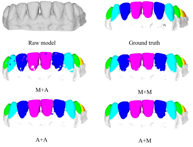
We also show the segmentation results of a typical example obtained by these variants in Fig. 5. In consistency with quantitative evaluations in Table 3, we can see that both M+A and M+M have more outliers than A+A and A+M, which further confirms that graph attention aggregation is more suitable for the C-stream. Besides, when comparing A+A with A+M, we also observe that A+M generates more precise segmentation on boundaries, which further confirms that graph max-pooling aggregation is more suitable for the N-stream.
5.3 Effectiveness of Feature-Fusion Strategy
As described in Section 3.3, the multi-scale high-level feature produced by C-stream and N-stream (i.e., and ) are fused to learn complementary information in our TSGCNet. To evaluate the effectiveness of this high-level feature fusion strategy, we compare the TSGCNet with another variant that is implemented by applying a low-level feature fusion strategy. Specifically, during the two-stream feature extraction stage, the output of the -th layer in both streams are concatenated (i.e., and are concatenated) as the input of the -th layer. This means that the C-stream and N-stream have the same input in the -th layer. We denote our original feature fusion strategy and the variant as H-fusion and L-fusion, respectively.
| Strategy | OA | mIoU |
|---|---|---|
| L-fusion | 93.28 | 85.49 |
| H-fusion | 95.25 | 88.99 |
We further compare the segmentation results of H-fusion and L-fusion, as shown in Table 4. From this table, it can be seen that the OA and mIoU of H-fusion is 1.97% and 3.50% higher than L-fusion, respectively. It is potentially because the premature feature fusion also confuses the learning of discriminative features. Besides, due to different properties between coordinates and normal vectors, the KNN graph built on the concatenated features may result in a random distribution of neighbors in real space, which tends to hamper the network to learn local-to-global information.
5.4 Limitations
Although our TSGCNet has achieved the leading performance in the task of 3D dental segmentation, it still has certain limitations. Most typically, TSGCNet cannot robustly handle special cases with 12 teeth. For example, we showed the segmentation result of one dental model with 12 teeth in Fig. 6, which can be seen that our TSGCNet generates many false predictions on T6 (indicated by the blue dotted circles). This can be possibly interpreted by the fact that the outermost tooth of 12-teeth dental models is annotated as T6, which is usually annotated as T7 in the normal dental models. To address this problem, including more 12-teeth cases as training samples would be considered in our future research.

6 Conclusion
A two-stream network, called TSGCNet, has been proposed in this paper to automatically segment individual tooth from 3D dental models acquired by intra-oral scanners. To eliminate the mutual confusion caused by mixed geometric inputs, the proposed TSGCNet apply two input-aware graph-learning streams to independently extract discriminative geometric features from coordinates and normal vectors, respectively. Feature representations produced by two different stream are then fused to learn complementary multi-view information for the end-to-end cell-wise prediction. An extensive comparison has been performed between our TSGCNet and other five state-of-the-art methods on a real-patient dataset, and the corresponding results demonstrate the superiority of our proposed method, especially for practically challenging cases.
References
- (1) Xiaozhi Chen, Huimin Ma, Ji Wan, Bo Li, and Tian Xia. Multi-view 3d object detection network for autonomous driving. In Proceedings of the IEEE Conference on Computer Vision and Pattern Recognition (CVPR), July 2017.
- (2) Angela Dai and Matthias Nießner. 3dmv: Joint 3d-multi-view prediction for 3d semantic scene segmentation. In Proceedings of the European Conference on Computer Vision (ECCV), 2018.
- (3) Ding, Xi, Liu, Shi-jian, Zou, Bei-ji, Liao, Sheng-hui, Liang, and Ye. Interactive tooth partition of dental mesh base on tooth-target harmonic field. Computers in Biology and Medicine, 56(Feb.):132–144, 4 2015.
- (4) Mingtao Feng, Liang Zhang, Xuefei Lin, Syed Zulqarnain Gilani, and Ajmal Mian. Point attention network for semantic segmentation of 3d point clouds. Pattern Recognition, 107:107446, 2020.
- (5) Farhad Ghazvinian Zanjani, David Anssari Moin, Bas Verheij, Frank Claessen, Teo Cherici, Tao Tan, and Peter H. N. de With. Deep learning approach to semantic segmentation in 3d point cloud intra-oral scans of teeth. volume 102 of Proceedings of Machine Learning Research, pages 557–571, London, United Kingdom, 08–10 Jul 2019. PMLR.
- (6) Benjamin Graham, Martin Engelcke, and Laurens van der Maaten. 3d semantic segmentation with submanifold sparse convolutional networks. In Proceedings of the IEEE Conference on Computer Vision and Pattern Recognition (CVPR), June 2018.
- (7) Li Jiang, Hengshuang Zhao, Shu Liu, Xiaoyong Shen, Chi-Wing Fu, and Jiaya Jia. Hierarchical point-edge interaction network for point cloud semantic segmentation. In Proceedings of the IEEE/CVF International Conference on Computer Vision (ICCV), October 2019.
- (8) Thomas Kronfeld, Thomas Kronfeld, David Brunner, David Brunner, Guido Brunnett, and Guido Brunnett. Snake-based segmentation of teeth from virtual dental casts. Computer-Aided Design and Applications, 7(2):221–233, 12 2010.
- (9) Yokesh Kumar, Ravi Janardan, Brent Larson, and Joe Moon. Improved segmentation of teeth in dental models. Computer-Aided Design and Applications, 8(2):211–224, 2011.
- (10) Truc Le, Giang Bui, and Ye Duan. A multi-view recurrent neural network for 3d mesh segmentation. Computers & Graphics, 66:103 – 112, 2017. Shape Modeling International 2017.
- (11) Truc Le and Ye Duan. Pointgrid: A deep network for 3d shape understanding. In Proceedings of the IEEE Conference on Computer Vision and Pattern Recognition (CVPR), June 2018.
- (12) Yangyan Li, Rui Bu, Mingchao Sun, Wei Wu, Xinhan Di, and Baoquan Chen. Pointcnn: Convolution on x-transformed points. In S. Bengio, H. Wallach, H. Larochelle, K. Grauman, N. Cesa-Bianchi, and R. Garnett, editors, Advances in Neural Information Processing Systems 31, pages 820–830. Curran Associates, Inc., 2018.
- (13) C. Lian, L. Wang, T. Wu, F. Wang, P. Yap, C. Ko, and D. Shen. Deep multi-scale mesh feature learning for automated labeling of raw dental surfaces from 3d intraoral scanners. IEEE Transactions on Medical Imaging, 39(7):2440–2450, 2020.
- (14) Chunfeng Lian, Li Wang, Tai-Hsien Wu, Mingxia Liu, Francisca Durán, Ching-Chang Ko, and Dinggang Shen. Meshsnet: Deep multi-scale mesh feature learning for end-to-end tooth labeling on 3d dental surfaces. In International Conference on Medical Image Computing and Computer-Assisted Intervention, pages 837–845. Springer, 2019.
- (15) Z. Liang, M. Yang, H. Li, and C. Wang. 3d instance embedding learning with a structure-aware loss function for point cloud segmentation. IEEE Robotics and Automation Letters, 5(3):4915–4922, 2020.
- (16) D. Maturana and S. Scherer. Voxnet: A 3d convolutional neural network for real-time object recognition. In 2015 IEEE/RSJ International Conference on Intelligent Robots and Systems (IROS), pages 922–928, 2015.
- (17) G. Pang and U. Neumann. 3d point cloud object detection with multi-view convolutional neural network. In 2016 23rd International Conference on Pattern Recognition (ICPR), pages 585–590, 2016.
- (18) Qi, Charles R., Su, Hao, Niessner, Matthias, Dai, Angela, Yan, Mengyuan, Guibas, and Leonidas J. Volumetric and multi-view cnns for object classification on 3d data. 3 2016.
- (19) Charles R. Qi, Hao Su, Kaichun Mo, and Leonidas J. Guibas. Pointnet: Deep learning on point sets for 3d classification and segmentation. In Proceedings of the IEEE Conference on Computer Vision and Pattern Recognition (CVPR), July 2017.
- (20) Charles Ruizhongtai Qi, Li Yi, Hao Su, and Leonidas J Guibas. Pointnet++: Deep hierarchical feature learning on point sets in a metric space. In I. Guyon, U. V. Luxburg, S. Bengio, H. Wallach, R. Fergus, S. Vishwanathan, and R. Garnett, editors, Advances in Neural Information Processing Systems 30, pages 5099–5108. Curran Associates, Inc., 2017.
- (21) Gernot Riegler, Ali Osman Ulusoy, and Andreas Geiger. Octnet: Learning deep 3d representations at high resolutions. In Proceedings of the IEEE Conference on Computer Vision and Pattern Recognition (CVPR), July 2017.
- (22) Chanjira Sinthanayothin and Wichit Tharanont. Orthodontics treatment simulation by teeth segmentation and setup. In 5th International Conference on Electrical Engineering/Electronics, Computer, Telecommunications and Information Technology (ECTI-CON 2008), vol.1, pages 81–84, Krabi, Thailand, 1 2008.
- (23) Kondo T., Foong K.W.C., and Ong S.H. Tooth segmentation of dental study models using range images. IEEE Transactions on Medical Imaging, 23(3):350–362, 5 2004.
- (24) Gusi Te, Wei Hu, Amin Zheng, and Zongming Guo. Rgcnn: Regularized graph cnn for point cloud segmentation. In Proceedings of the 26th ACM International Conference on Multimedia, MM ’18, page 746–754, New York, NY, USA, 2018. Association for Computing Machinery.
- (25) S. Tian, N. Dai, B. Zhang, F. Yuan, Q. Yu, and X. Cheng. Automatic classification and segmentation of teeth on 3d dental model using hierarchical deep learning networks. IEEE Access, 7:84817–84828, 2019.
- (26) Chu Wang, Babak Samari, and Kaleem Siddiqi. Local spectral graph convolution for point set feature learning. In Proceedings of the European Conference on Computer Vision (ECCV), September 2018.
- (27) Lei Wang, Yuchun Huang, Yaolin Hou, Shenman Zhang, and Jie Shan. Graph attention convolution for point cloud semantic segmentation. In Proceedings of the IEEE/CVF Conference on Computer Vision and Pattern Recognition (CVPR), June 2019.
- (28) Peng-Shuai Wang, Yang Liu, Yu-Xiao Guo, Chun-Yu Sun, and Xin Tong. O-cnn: Octree-based convolutional neural networks for 3d shape analysis. ACM Transactions on Graphics (SIGGRAPH), 36(4), 2017.
- (29) Yue Wang, Yongbin Sun, Ziwei Liu, Sanjay E. Sarma, Michael M. Bronstein, and Justin M. Solomon. Dynamic graph cnn for learning on point clouds. ACM Trans. Graph., 38(5), Oct. 2019.
- (30) Z. Wang and F. Lu. Voxsegnet: Volumetric cnns for semantic part segmentation of 3d shapes. IEEE Transactions on Visualization and Computer Graphics, 26(9):2919–2930, 2020.
- (31) Nonlapas Wongwaen and Chanjira Sinthanayothin. Computerized algorithm for 3d teeth segmentation. In 2010 International Conference on Electronics and Information Engineering. v.1, pages V1–277–V1–280, Kyoto, Japan, 1 2010. IEEE.
- (32) Kan Wu, Li Chen, Jing Li, and Yanheng Zhou. Tooth segmentation on dental meshes using morphologic skeleton. Computers & graphics, 38(Feb.):199–211, 5 2014.
- (33) Wenxuan Wu, Zhongang Qi, and Li Fuxin. Pointconv: Deep convolutional networks on 3d point clouds. In Proceedings of the IEEE/CVF Conference on Computer Vision and Pattern Recognition (CVPR), June 2019.
- (34) Zhirong Wu, Shuran Song, Aditya Khosla, Fisher Yu, Linguang Zhang, Xiaoou Tang, and Jianxiong Xiao. 3d shapenets: A deep representation for volumetric shapes. In Proceedings of the IEEE Conference on Computer Vision and Pattern Recognition (CVPR), June 2015.
- (35) Zhuyang Xie, Junzhou Chen, and Bo Peng. Point clouds learning with attention-based graph convolution networks. Neurocomputing, 402:245 – 255, 2020.
- (36) Xu, Xiaojie, Liu, Chang, Zheng, and Youyi. 3d tooth segmentation and labeling using deep convolutional neural networks. IEEE transactions on visualization and computer graphics, 25(7):2336–2348, 1 2019.
- (37) Mingye Xu, Zhipeng Zhou, and Yu Qiao. Geometry sharing network for 3d point cloud classification and segmentation. In AAAI, pages 12500–12507, 2020.
- (38) Ma Yaqi and Li Zhongke. Computer aided orthodontics treatment by virtual segmentation and adjustment. In 2010 International Conference on Image Analysis and Signal Processing (IASP 2010), pages 336–339, Zhejiang, China, 1 2010. IEEE.
- (39) Haoxuan You, Yifan Feng, Rongrong Ji, and Yue Gao. Pvnet: A joint convolutional network of point cloud and multi-view for 3d shape recognition. In Proceedings of the 26th ACM International Conference on Multimedia, MM ’18, page 1310–1318, New York, NY, USA, 2018. Association for Computing Machinery.
- (40) Tianran Yuan, Wenhe Liao, Ning Dai, Xiaosheng Cheng, and Qing Yu. Single-tooth modeling for 3d dental model. International Journal of Biomedical Imaging, 2010, 2010.
- (41) Mingxi Zhao, Lizhuang Ma, Wuzheng Tan, and Dongdong Nie. Interactive tooth segmentation of dental models. In 2005 IEEE Engineering in Medicine and Biology 27th Annual Conference, pages 654–657. IEEE, 2006.