Alternative experimental ways to access entropy production

We first review the measures of irreversibility established within the so-called quantum Jarzynski’s protocol An2015; Huber2008; Campisi2011; Batalhao2014; Heyl2012; Dorner2013; Mazzola2013, schematically presented in Fig. 1(a). After having thermalized with a heat reservoir at temperature $T$, a quantum system starts in the thermal equilibrium state $\zeta$ with inverse temperature $\beta=\left(k_{\text{B}}T\right)^{-1}$, also known as thermodynamic beta, where $k_{\text{B}}$ is the Boltzmann’s constant. The system is first driven out of equilibrium through a unitary operation $U$, to the non-equilibrium state $\rho_{\text{f}}$ (here and in the following the subscript f labels quantities at the end of the evolution). To be treated as a unitary, $U$ is assumed to be performed swiftly compared to the system relaxation. Then, the system relaxes back to the thermal state $\zeta$. This last step causes the whole process to be irreversible. The entropy production ${\Sigma}$ is proportional to the amount of heat $Q$ dissipated by the system along its thermalization, ${\Sigma}=\beta Q$. It is shown to equal the relative entropy $D(\rho_{\text{f}}||\zeta)$, also known as quantum divergence, quantifying the non-negative distance between the two states. For states $\rho$ and $\sigma$, it is defined as $D(\rho||\sigma)=-\mathrm{Tr}[\rho\ln\sigma]-S(\rho)$, where $S(\rho)$ is the von Neumann entropy of state $\rho$ Vedral2002. This provides a first intuitive flavour for the EP: the farther the system is brought away from equilibrium, the larger the entropy production.

Another meaning for the EP is acquired by the attempt to reverse the forward evolution $U$. For this purpose we complete the above protocol with the time-reversed unitary operation $\tilde{U}$. In general, unitary operations are considered as reversible: from an operational point of view this presupposes the ability to generate the backward evolution $U^{\dagger}=\tilde{U}$ (here and in the following the symbol $\sim$ denotes the backward quantities). In the absence of the intermediate thermalization, this backward evolution would bring the system back to its initial state. The presence of the intermediate irreversible thermalization is the reason why the process cannot be reversed. EP is shown to equal the relative entropy $D(\zeta||\tilde{\rho}_{\text{f}})$ of the initial thermal state with respect to the final state $\tilde{\rho}_{\text{f}}$ of this backward evolution. This is also intuitive: the lower our ability to time-reverse the evolution, the larger the entropy production.

Finally, the concept of EP can be extended at the level of single realizations, that corresponds to two-point quantum trajectories in the present quantum Jarzynski’s protocol. Each trajectory $\gamma$ is defined by the outcomes of energy measurements performed at the beginning and at the end of the forward protocol, while $\tilde{\gamma}$ stands for its time-reversed counterpart, as introduced in the pioneering two-point energy measurement (TPEM) scheme (Esposito2009; Campisi2011; Binderbook2018). The stochastic EP is defined as ${\sigma}[\gamma]=\ln(p(\gamma)/p(\tilde{\gamma}))$ and compares the probability $p(\gamma)$ for $\gamma$ to be realized in the forward protocol and the probability $p(\tilde{\gamma})$ for the corresponding $\tilde{\gamma}$ in the backward protocol Landi2020. This expression provides us with another intuitive way to quantify irreversibility at the level of single trajectories. Although ${\sigma}[\gamma]$ can take negative values, its average ${\Sigma}$ over all possible trajectories is non-negative by convexity of the exponential, in agreement with the SLT.

From this brief review, it appears that EP can be captured owing to various operational resources and, in particular, to the ability to access average or stochastic physical quantities as well as to run an evolution forward and backward. In what follows, we systematically employ these different approaches of EP to a basic protocol of an information-powered fridge. More specifically, the system is measured by a controller (readout $R$) and its further unitary evolution $U^{(k)}$ is set by the readout outcome $k$, thus leading to several different evolution branches of the feedback-controlled system, see Fig. 1(b). Along with the two measurements forming the TPEM scheme the readout outcome also contributes to the definition of the quantum trajectories. For the sake of clarity, we first detail the non-autonomous description of the protocol, where the feedback uses information encoded on a classical memory of the external controller. Then, we focus on the autonomous description, i.e., for a fully closed system as reported in Ref. Luis2020.

Figure 2 illustrates a non-autonomous description of the Maxwell’s demon experiment studied in this paper. We consider a qubit Q and a cavity C. Their interaction is controlled by a third system further dubbed demon and denoted by D. In this description, D features a classical entity, performing a local projective measurement on Q in its energy basis and storing its result in a classical memory. The two measurement outcomes are then exploited in the feedback loop (readout followed by feedback), that conditionally acts on the joint QC system. Namely, they trigger a unitary system evolution $U^{(1)}=V$ for $k=1$ and no interaction, i.e., the identity $U^{(0)}=\mathbb{I}$, for $k=0$. All the EP expressions derived in this and the next section are also valid for more general settings, with two arbitrary systems Q and C.

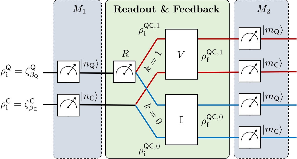
We first consider the average evolution of the joint QC system and use the density matrix approach to describe its state. Initially, Q and C start at the local thermal equilibrium state $\rho_{\text{i}}^{\textsf{QC}}=\zeta_{\beta_{\textsf{Q}}}^{\textsf{Q}}\otimes\zeta_{\beta_{\textsf{C}}}^{\textsf{C}}$, where $\zeta_{\beta_{j}}^{j}=\exp[-\beta_{j}\left(H^{j}-F^{j}\right)]$ are the Gibbs states. For each system $j\in\{\textsf{Q},\textsf{C}\}$, $H^{j}$ is the local Hamiltonian and $F^{j}=-(1/\beta_{j})\ln\text{Tr}\big[e^{-\beta_{j}H^{j}}\big]$ is the equilibrium free energy. The internal energy of system $j$ in state $\rho^{j}$ is given by $\mathcal{U}^{j}=\text{Tr}_{j}\left[H^{j}\rho^{j}\right]$. Next, D performs a projective measurement (i.e., demon readout) on the system. The measurement outcome $k$ projects QC onto the state $\rho_{\text{i}}^{\textsf{QC},k}$ with probability $p(k)$. Then, D stores the outcome $k$ and induces the unitary feedback operation $U^{(k)}$ between Q and C depending on $k$. There are thus several distinct branches, labelled by $k$, of the possible unitary evolution of the system. The final QC states and their average over all measurement outcomes read $\rho_{\text{f}}^{\textsf{QC},k}=U^{(k)}\rho_{\text{i}}^{\textsf{QC},k}[U^{(k)}]^{\dagger}$ and $\rho_{\text{f}}^{\textsf{QC}}=\sum_{k}p(k)\rho_{\text{f}}^{\textsf{QC},k}$, respectively. The relaxation of the non-equilibrium state $\rho_{\text{f}}^{\textsf{QC}}$ towards the initial thermal product state gives rise to the entropy production. The demon’s memory, on the other hand, does not relax and hence does not produce entropy. This leads to our first expression of EP:

where $\Delta\beta={\beta_{\textsf{C}}}-{\beta_{\textsf{Q}}}$, $Q^{\textsf{C}}=\sum_{k}p(k)\Delta\mathcal{U}^{\textsf{C},k}$ is the heat absorbed by C, $\Delta\mathcal{U}^{\textsf{C},k}$ is the energy change of C during the feedback operation in branch $k$, and ${\langle{I}\rangle}=H[p(k)]=-\sum_{k}p(k)\ln p(k)$ is the Shannon entropy of the readout measurement. We use the fact that ${Q^{\textsf{Q}}}=-{Q^{\textsf{C}}}$ for a closed system and an energy-preserving readout, see Appendix A. If there was no feedback action ($U^{(1)}=\mathbb{I}$), ${\Sigma_{1}}$ would reduce to the well-known classical expression ${\Sigma}=\Delta\beta{Q}$ (Landi2020), quantifying the entropic counterpart of the heat exchanged between two systems. In addition to this exchange term, Eq.(1) explicitly involves an informational contribution. This is in agreement with the pioneering expressions of the SLT in the presence of a feedback control that were obtained by explicitly taking the demon’s physical memory into account (Sagawa2008; Sagawa2009; Maruyama2009).

An alternative, second expression for the EP can be obtained starting from the following identity for an arbitrary state $\rho$: $D(\rho||\zeta)=\beta[\mathcal{U}(\rho)-F]-S(\rho)$. Writing the heat in (1) in terms of the quantum divergence we obtain

where $\rho_{\text{f}}^{\textsf{QC},k}$ is the final QC state conditioned on $k$, see Appendix A. This expression can be interpreted as follows. The entropy production for a thermalization process is known to be given by the quantum divergence of the initial state with respect to the final thermal one (Deffner2011). For a given $k$, the entropy produced during the thermalization equals $D\!\left(\rho_{\text{f}}^{\textsf{QC},k}||\zeta_{\beta_{\textsf{Q}}}^{\textsf{Q}}\otimes\zeta_{\beta_{\textsf{C}}}^{\textsf{C}}\right)$. The total EP is, therefore, the average of such a conditional EP, associated to each branch $k$, over all readout outcomes.

The expressions ${\Sigma_{1}}$ and ${\Sigma_{2}}$ rely on the physical quantities provided by the forward protocol only. A third expression containing information also from the backward protocol can be obtained as well. For each branch $k$, the backward process is defined by the application of the time-reversed unitary $\tilde{U}^{(k)}=[U^{(k)}]^{\dagger}$ on the state after the thermalization, while the demon’s memory remains unchanged. Thus, the probability of applying $\tilde{U}^{(k)}$ is given by the probability $p(k)$ of ending up in the forward branch $k$. Starting from (2) we show in Appendix A that

where $\tilde{\rho}_{\text{f}}^{\textsf{QC},k}$ is the QC state of the backward protocol of the branch $k$ after the backward evolution $\tilde{U}^{(k)}$. This expression for the EP also comes in the form of the average over the outcomes of the readout measurement. It is a generalization of the equation obtained in Ref. (Batalhao2015), where there is no feedback control being considered.

The system evolution can also be described stochastically by means of individual quantum trajectories. All thermodynamic quantities become trajectory-dependent, providing a finer description of the system dynamics. In the spirit of the TPEM scheme, the definition of our quantum trajectories involve the initial and final energy states of the joint QC system, respectively denoted $\ket{{n_{\textsf{Q}}},{n_{\textsf{C}}}}$ and $\ket{{m_{\textsf{Q}}},{m_{\textsf{C}}}}$. In the present case where the dynamics generates no coherence in the energy basis, these states can be accessed by two energy measurements $M_{1}$ and $M_{2}$ respectively performed at the beginning and at the end of the feedback loop, of respective outcomes $\{{n_{\textsf{Q}}},{n_{\textsf{C}}}\}$ and $\{{m_{\textsf{Q}}},{m_{\textsf{C}}}\}$.

The probability of the measurement outcomes $\{{n_{\textsf{Q}}},{n_{\textsf{C}}}\}$ is $p({n_{\textsf{Q}}},{n_{\textsf{C}}})=p({n_{\textsf{Q}}})p({n_{\textsf{C}}})$, where the probabilities $p(n_{j})$ are the Boltzmann weights of the initial uncorrelated thermal states. The demon readout R of outcome $k$ conditions the QC evolution $U^{(k)}$ between $M_{1}$ and $M_{2}$. For the ideal readout, the state $\ket{{n_{\textsf{Q}}}}$ deterministically sets the value of $k$. In a more general case, we can consider a conditional probability $p(k|{n_{\textsf{Q}}})$ of the readout outcome $k$ accounting for possible readout limitations, such as non-projective measurement or detection errors. Eventually, the trajectory $\gamma$ is defined by a unique set of the initial states $\ket{{n_{\textsf{Q}}},{n_{\textsf{C}}}}$, the system evolution branch $k$, and the final state $\ket{{m_{\textsf{Q}}},{m_{\textsf{C}}}}$. The forward trajectory probability distribution $p(\gamma)$ is given by the probability of getting the set of outcomes $\gamma=\{{n_{\textsf{Q}}},k,{n_{\textsf{C}}},{m_{\textsf{Q}}},{m_{\textsf{C}}}\}$ and it explicitly reads

The total number of all possible trajectories is $d_{\textsf{Q}}^{2}\times d_{\textsf{C}}^{2}\times d_{\textsf{Q}}$, where $d_{j}$ is the size of the Hilbert space of the system $j$. The last contribution, $d_{\textsf{Q}}$, comes from the fact that the external controller (demon) must contain $d_{\textsf{Q}}$ distinguishable states to encode the measurement outcomes.

We now turn our attention to the distribution of the backward trajectories. As mentioned above, the backward process in each reverse branch $k$ is generated by the time-reversed unitary $\tilde{U}^{(k)}$. The backward trajectory $\tilde{\gamma}$ is defined by the set of parameters $\{{n_{\textsf{Q}}},k,{n_{\textsf{C}}},{m_{\textsf{Q}}},{m_{\textsf{C}}}\}$ and is the counterpart of the forward trajectory $\gamma$ labelled by the same indices. Similarly to the forward protocol, the probability distribution of the backward trajectories is given by

where ${p_{\text{b}}}({n_{\textsf{Q}}},{n_{\textsf{C}}}|{m_{\textsf{Q}}},k,{m_{\textsf{C}}})$ is the conditional probability of the final backward state. The initial backward probabilities ${p_{\text{b}}}({m_{\textsf{Q}}})$ and ${p_{\text{b}}}({m_{\textsf{C}}})$ are determined from the corresponding initial Gibbs states. The probability $p(k)$ of the backward branch $k$ equals the probability of the readout outcome $k$ in the forward protocol.

Given the probabilities of the forward trajectory $\gamma$ and of the corresponding backward trajectory $\tilde{\gamma}$, the stochastic EP is defined as $\sigma[\gamma]=\ln\big(p(\gamma)/p(\tilde{\gamma})\big)$. The average EP computed over all $\gamma$’s is then given by (Landi2020)

where the relative entropy $D$ is computed between probability distributions $p(\gamma)$ and $p(\tilde{\gamma})$. Note that for classical distributions $p_{n}$ and $q_{n}$, $D$ is defined by the Kullback-Leibler divergence: $D\left(p||q\right)=\sum_{n}p_{n}\ln\left(p_{n}/q_{n}\right)$ (Coverbook2006), which is equivalent to the quantum divergence between two states whose density matrices are diagonal in the same basis. The expression ${\Sigma_{4}}$ quantifies the irreversibility by comparing the stochastic trajectories of the forward and backward protocols. Notably, its computation requires no knowledge on the actual physical states defining the trajectories, but needs only the ability to distinguish different trajectories in order to properly access their probabilities.

We define as $p\left(\sigma\right)=\sum_{\gamma}p\left(\gamma\right)\delta_{\sigma,\sigma\left[\gamma\right]}$ and ${p_{\text{b}}}(\sigma)=\sum_{\gamma}p\left(\tilde{\gamma}\right)\delta_{\sigma,\sigma\left[\gamma\right]}$ the total probability of the forward and backward trajectories, respectively, contributing to the value $\sigma$ of EP, where $\delta_{a,b}$ is the Kronecker delta. With these two probability distributions one can easily show the detailed fluctuation relation: $\exp(\sigma)=p(\sigma)/{p_{\text{b}}}(\sigma)$. By averaging over all possible values of $\sigma$ we obtain

The stochastic entropy production $\sigma[\gamma]$ for each trajectory $\gamma$, required for computing ${\Sigma_{5}}$, can be obtained as

see Appendix A. Here, $Q^{j}[\gamma]$ is the stochastic heat received by the system $j\in\{\textsf{Q},\textsf{C}\}$ and $I[\gamma]=-\ln p(k)$ is the stochastic information extracted from the readout measurement. On the contrary to ${\Sigma_{4}}$, the expression ${\Sigma_{5}}$ compares the forward and backward probability contributions to the EP, even if $\sigma[\gamma]$ is degenerate for some trajectories. Thus, despite the obvious similarity of the mathematical expressions, ${\Sigma_{4}}$ and ${\Sigma_{5}}$ differ appreciably with respect to the information required for their computation.

In the non-autonomous description the demon D has been treated as a classical feedback loop, involving a measurement and a conditional action on the QC system. The demon’s influence has been taken into account through the measurement outcome probability $p(k)$ quantifying the information extracted by D from the system Q. Alternatively, we can also consider a global QDC system incorporating D with the demon feedback action being part of a global unitary evolution of this closed system. For the remainder of this section we apply to our experiment the autonomous demon description reported in Ref. Luis2020. The equivalent quantum circuit for the forward protocol corresponding to a two-level (qubit) system Q is depicted in Fig. 4. The demon, also assumed to be a qubit without loss of generality, starts in the pure reference state $\ket{1_{\textsf{D}}}$. Both the readout and the feedback operations are dynamically implemented by means of global unitaries on the total QDC system. The projective readout in the energy basis of Q is replaced by a controlled NOT (CNOT) gate. It transforms the initial state of D into $\ket{0_{\textsf{D}}}$ if the state of Q is $\ket{0_{\textsf{Q}}}$. After the CNOT gate, a controlled unitary operation between Q and C is performed to appropriately implement the feedback action. As expected, the reduced QC state after this operation is $\sum_{k}p(k)\rho_{\text{f}}^{\textsf{QC},k}$, which is the average final state $\rho_{\text{f}}^{\textsf{QC}}$ of the protocol described in Sec. II.3.

Our final expression for the EP comes from the analysis of the closed QDC system with the demon D explicitly included as a third quantum system. We show in Appendix A that

where $I^{\textsf{QC}:\textsf{D}}=D\left(\rho^{\textsf{QDC}}||\rho^{\textsf{QC}}\!\otimes\!\rho^{\textsf{D}}\right)$ is the mutual information between QC and D, while $\Delta_{\text{fb}}$ denotes the information change during the feedback step, i.e., before and after the controlled unitary gate. We consider here the ideal readout, i.e., $p(k|{n_{\textsf{Q}}})=\delta_{k,{n_{\textsf{Q}}}}$. This relation is a generalization to our current protocol of the expression first derived in Ref. (Luis2020). It comes directly from the entropy conservation of the global QDC system for the closed evolution depicted in Fig. 4.

Since the correlations before the feedback step are given by the Shannon entropy $H[p(k)]$, substituting (9) into (1) we obtain

It clearly shows that the EP has two contributions. The divergence quantifies the entropy produced in the thermalization process for the QC system starting in the state $\rho_{\text{f}}^{\textsf{QC}}$. The final mutual information between the two subsystems QC and D quantifies the amount of entropy produced by erasing all correlations between them, due to the thermalization. This result evidences that there is an entropic cost for erasing correlations Landi2020; Camati2021.

Table 1 summarizes the six alternative expressions for the entropy production along with additional information on the underlying protocols and the statistical nature of the required physical quantities. Expressions $\Sigma_{1}$, $\Sigma_{2}$ and $\Sigma_{6}$ are based on the data extracted exclusively from the forward protocol. The other expressions require the execution and analysis of the backward protocol as well. We can distinguish three types of physical quantities showing up in different expressions: expressions $\Sigma_{1}$ and $\Sigma_{6}$ can be computed using information on the average initial and final states of the system (“averaged”). Expressions $\Sigma_{2}$ and $\Sigma_{3}$ are based on data averaged over different readout outcomes, thus requiring the discrimination of different evolution branches (“branched”). Finally, to compute expressions $\Sigma_{4}$ and $\Sigma_{5}$ we have to resolve individual trajectories (“stochastic”).

Describing the same physical quantity, all these expressions are equivalent under the restriction of ideal unitary evolutions and ideal projective measurements, which have been used for their derivation. In the presence of realistic deviations from the idealized scenario, they start to differ, as will be shown in the next Section. For diagonal states, as considered here, only the expressions $\Sigma_{2}$ and $\Sigma_{6}$ stay mathematically identical and provide the same EP value irrespective of the evolution imperfections, see Appendix B.

We measure the entropy production in the Maxwell’s demon system described by the quantum circuit in Fig. 4 and realized in a cavity QED setup Luis2020. Qubit Q and two-level demon D are simultaneously encoded into three adjacent circular Rydberg states of a single Rubidium atom A (with principle quantum numbers $49$, $50$ and $51$ corresponding to atomic states $\ket{f}$, $\ket{g}$ and $\ket{e}$, respectively). The mapping between the logical states of the QD system and the physical states of A is the following: $\ket{1_{\textsf{Q}},\!1_{\textsf{D}}}=\ket{e}$, $\ket{0_{\textsf{Q}},\!1_{\textsf{D}}}=\ket{g}$, and $\ket{0_{\textsf{Q}},\!0_{\textsf{D}}}=\ket{f}$. According to the Maxwell’s demon circuit, see Fig. 4, the state $\ket{0_{\textsf{Q}},\!1_{\textsf{D}}}$ is never populated and does not need to be encoded in a particular physical state of A. The system C is realized with a high-quality superconducting microwave cavity resonant with the atomic $\ket{g}$–$\ket{e}$ transition at $51$ GHz and far detuned from the $\ket{g}$–$\ket{f}$ transition at $54$ GHz.

The basic experimental setup is schematically presented in Fig. 5. Individual flying Rydberg atoms exit the preparation zone B in the state $|g\rangle$. To prepare the state $|e\rangle$ a resonant microwave pulse is applied in R${}_{\textsf{Q}}$ by means of the microwave source S_eg. Its amplitude and duration are adjusted to realize a Rabi $\pi$-pulse between $|g\rangle$ and $|e\rangle$. The demon readout is implemented by deterministically flipping the atomic states $\ket{g}$ and $\ket{f}$ before A enters C. This operation is induced by the microwave source S_gf resonant with the $\ket{g}$–$\ket{f}$ transition and adjusted to maximize the atomic population transfer.

The atom-cavity interaction is controlled by an electric field applied across C by the voltage source V via Stark-tuning the atomic frequency. The demon feedback is implemented by a resonant interaction between A and C based on the adiabatic passage technique. It allows for the efficient population transfer between the AC states $\ket{e,n}$ and $\ket{g,n+1}$ independent of the cavity photon number $n$. Energy conservation prevents the coupling of the joint ground state $\ket{g,0}$ to other states.

The atomic states are directly measured by a field-ionisation detector M providing us with the final qubit and demon states, $\ket{{m_{\textsf{Q}}}}$ and $\ket{{m_{\textsf{D}}}=k}$, respectively. The cavity photon-number state $\ket{{m_{\textsf{C}}}}$ is probed by a sequence of several tens of atoms interacting with C in the dispersive regime and performing a quantum non-demolition (QND) measurement of its photon number Guerlin07.

Each of the six EP expressions can be experimentally accessed by running the Maxwell’s demon circuit and measuring physical quantities entering these expressions using measurement strategies properly adapted to each quantity. For instance, the cavity energy change $Q^{\textsf{C}}$, required to compute ${\Sigma_{1}}$, can be obtained by comparing the average initial and final photon number in the cavity without the need to resolve different numbers. However, in order to significantly reduce the overall data acquisition time and to address all expressions at once we have decided to record the complete statistics of individual trajectories in the forward and backward protocols of the Maxwell’s demon circuit. Knowing the initial and final states of each trajectory as well as their occurrence probability allows us to compute any physical quantity appearing in the EP expressions, as will be shown below.

In order to get the EP for any initial temperature of Q and C without increasing the overall experimental time, we have decided to replace the combination of the initial thermal state preparation and the first projective measurement of the TPEM scheme with the direct preparation of the QDC system in the pure energy eigenstate $\ket{{n_{\textsf{Q}}},1_{\textsf{D}},{n_{\textsf{C}}}}$. The different thermal states are then taken into account by using the corresponding theoretical probability distributions $p({n_{\textsf{Q}}})$ and $p({n_{\textsf{C}}})$. We have shown in Ref. Luis2020 that the experimental Gibbs’ states of Q and C of given temperatures ${\beta_{\textsf{Q}}}$ and ${\beta_{\textsf{C}}}$ can be experimentally prepared and measured to be in good agreement with the theoretical distributions $p({n_{\textsf{Q}}})$ and $p({n_{\textsf{C}}})$.

Summarizing, in our basic experimental sequence we initially prepare the QDC system in the pure energy eigenstate $\ket{{n_{\textsf{Q}}},1_{\textsf{D}},{n_{\textsf{C}}}}$ and measure the probability of its final state $\ket{{m_{\textsf{Q}}},k,{m_{\textsf{C}}}}$ after the feedback evolution. In this way we obtain the conditional probability $p({m_{\textsf{Q}}},k,{m_{\textsf{C}}}|{n_{\textsf{Q}}},{n_{\textsf{C}}})$ of the trajectory $\gamma=\{{n_{\textsf{Q}}},k,{n_{\textsf{C}}},{m_{\textsf{Q}}},{m_{\textsf{C}}}\}$. Note that the initial demon state is always $\ket{1_{\textsf{D}}}$ and thus does not enter into the trajectory definition. Finally, for any temperature ${\beta_{\textsf{Q}}}$ and ${\beta_{\textsf{C}}}$ with the corresponding $p({n_{\textsf{Q}}})$ and $p({n_{\textsf{C}}})$ we compute $p(\gamma)$ using Eq. (4).

In this work we consider, without loss of generality, the constant cavity temperature of $2.8$ K and the qubit temperature varying such that the relative inverse temperature $\delta\tilde{\beta}=1-{\beta_{\textsf{Q}}}/{\beta_{\textsf{C}}}\in[-6,6]$. Since the populations of the photon-number states larger than 3 are negligible for this temperature (the mean thermal photon number is $0.71$), we restrict ${n_{\textsf{C}}}$ to values from $0$ to $3$ only.

The vacuum state $\ket{{n_{\textsf{C}}}=0}$ of C is prepared by sending through its mode a beam of resonant atoms in state $\ket{g}$. They absorb all photons from C thus cooling it into the vacuum. The state $\ket{{n_{\textsf{C}}}=1}$ with one photon is excited from the vacuum by using one atom in state $\ket{e}$ and forcing it to resonantly emit a photon into C. The preparation of larger photon-number states are realized by the QND projection of a small coherent field Guerlin07. We first inject into C a coherent field with about $3$ photons on average. Then, we perform the QND measurement, randomly resulting in different photon-number states. Finally, we post-select and sort all trajectories with the initial projected states $\ket{{n_{\textsf{C}}}=2}$ and $\ket{{n_{\textsf{C}}}=3}$.

The final QDC state is measured independently on each ensemble of quantum trajectories with the same initial state $\ket{{n_{\textsf{Q}}},{n_{\textsf{C}}}}$. The final detection of A gives us the conditional probability $p({m_{\textsf{Q}}},k|{n_{\textsf{Q}}},{n_{\textsf{C}}})$. The cavity photon-number probability is reconstructed on the ensemble of trajectories Metillon19 with the same initial and final QD state. In this way we obtain the conditional distribution $p({m_{\textsf{C}}}|{n_{\textsf{Q}}},{n_{\textsf{C}}},{m_{\textsf{Q}}},k)$ and compute $p({m_{\textsf{Q}}},k,{m_{\textsf{C}}}|{n_{\textsf{Q}}},{n_{\textsf{C}}})=p({m_{\textsf{C}}}|{n_{\textsf{Q}}},{n_{\textsf{C}}},{m_{\textsf{Q}}},k)\,p({m_{\textsf{Q}}},k|{n_{\textsf{Q}}},{n_{\textsf{C}}})$. The procedure of the state preparation and detection, along with all measured probabilities, is presented in detail in Appendix D. The probability of the trajectory $\gamma=\{{n_{\textsf{Q}}},{n_{\textsf{C}}},{m_{\textsf{Q}}},k,{m_{\textsf{C}}}\}$ for each ${\beta_{\textsf{Q}}}$ then equals $p(\gamma)=p({m_{\textsf{Q}}},k,{m_{\textsf{C}}}|{n_{\textsf{Q}}},{n_{\textsf{C}}})\,p({n_{\textsf{Q}}})\,p({n_{\textsf{C}}})$. A similar procedure is realized to obtain the probability distribution $p(\tilde{\gamma})$ of the backward trajectories. The set of probabilities $\{p(\gamma)\}$ and $\{p(\tilde{\gamma})\}$ are used in the following to compute all expressions for the entropy production, as explained below for each EP expression.

Figure 6 shows the temperature dependence of the entropy production ${\Sigma}$ computed from the six expressions. Dotted lines correspond to the theoretical values for the ideal QDC system as presented by the quantum circuit in Fig. 4. As expected, they coincide for all expressions, showing their fundamental equivalence. For large negative $\delta\tilde{\beta}$ (i.e., the qubit state close to $\ket{0_{\textsf{Q}}}$), the probability for Q to be in $\ket{1_{\textsf{Q}}}$ is small making the QC interaction after the demon readout unlikely. In this limit, the QC state stays almost unchanged reducing the entropy production to zero. For large positive $\delta\tilde{\beta}$ (i.e., the qubit state close to $\ket{1_{\textsf{Q}}}$), ${\Sigma}$ linearly increases with $\delta\tilde{\beta}$, see Appendix C. Since Q is mostly in $\ket{1_{\textsf{Q}}}$, the QC interaction is extremely likely, pushing the QC state further away from the initial thermal one and, consequently, producing more entropy.

The solid lines in Fig. 6 are computed from the experimental results using the expressions ${\Sigma_{1}}$ to ${\Sigma_{6}}$ for panels (a) to (f), respectively. The deviation from the ideal curves is due to experimental imperfections. The most significant imperfections are the preparation error ${\epsilon_{\text{prep}}}$ of the initial atomic states, the errors of the readout (${\epsilon_{\text{read}}}$) and feedback (${\epsilon_{\text{feed}}}$) operations and the discrimination error ${\epsilon_{\text{meas}}}$ of the atomic state measurement, see Appendix E for details. The errors ${\epsilon_{\text{read}}}$ and ${\epsilon_{\text{feed}}}$ modify the system evolution. They change the entropy production and influence equally all experimentally obtained ${\Sigma}$. Namely, the imperfect readout allows for the non-negligible QC interaction even for Q prepared in $\ket{0_{\textsf{Q}}}$ resulting in the non-zero ${\Sigma}$ for $\delta\tilde{\beta}\ll 0$. On the other hand, the imperfect feedback reduces the probability for the QC interaction for Q prepared in $\ket{1_{\textsf{Q}}}$, thus decreasing ${\Sigma}$ for $\delta\tilde{\beta}\gg 0$. The errors ${\epsilon_{\text{prep}}}$ and ${\epsilon_{\text{meas}}}$ mix the labels of the detected quantum trajectories. Since different expressions are based on different combinations of experimental data, these errors have, in general, a different effect on the different expressions of ${\Sigma}$. Other imperfections, like atom and cavity relaxations, have a minor effect on the TPEM scheme and are listed in Appendix F.

The computation of the first expression, ${\Sigma_{1}}$, given by (1) and presented in Fig. 6(a), starts by computing the stochastic heat change $Q^{\textsf{Q}}[\gamma]$ of Q for each trajectory $\gamma$. By averaging over all trajectories we get $Q^{\textsf{Q}}$. The probability $p(k=1)$ is given by the probability to finally detect D in the state $\ket{1_{\textsf{D}}}$ and equals the sum of $p(\gamma)$ over all trajectories with $k=1$. Here, we have used only the data from the atomic state detection of the forward protocol (i.e., no information on the cavity state is required). It is also noteworthy that the measured ${\Sigma_{1}}$ is higher than ${\Sigma}$ based on other expressions. Ideally, the Shannon entropy ${\langle{I}\rangle}$ goes to zero for large negative and positive $\delta\tilde{\beta}$ when the demon state after the readout is a pure quantum state, $\ket{1_{\textsf{D}}}$ or $\ket{0_{\textsf{D}}}$, respectively. However, due to the imperfect atomic state measurement ${\epsilon_{\text{meas}}}$, ${\langle{I}\rangle}$ is bound from below by $H[{\epsilon_{\text{meas}}}]$ thus shifting ${\Sigma_{1}}$ up, as seen in Fig. 6(a).

The state $\rho_{\text{f}}^{\textsf{QC},k}$ in the expression ${\Sigma_{2}}$ is obtained from the final probability distribution $p({m_{\textsf{Q}}},k,{m_{\textsf{C}}})$. The product Gibbs state $\zeta_{\beta_{\textsf{Q}}}^{\textsf{Q}}\otimes\zeta_{\beta_{\textsf{C}}}^{\textsf{C}}$ is set by temperatures ${\beta_{\textsf{Q}}}$ and ${\beta_{\textsf{C}}}$. The probability $p(k)$ is obtained in the same way as for ${\Sigma_{1}}$. Therefore, the current expression is based solely on the forward protocol after averaging the quantum trajectories into $\rho_{\text{f}}^{\textsf{QC},k}$. The experimental temperature dependence of ${\Sigma_{2}}$ is shown in Fig. 6(b).

Figure 6(c) presents the expression ${\Sigma_{3}}$ based on the analysis of the backward protocol with two branches, $k\!=\!0$ and $k\!=\!1$. It mainly relies on the backward trajectories, except for the value of $p(k)$ for the demon state extracted from the forward protocol. This expression shows the largest deviation from the ideal case for $\delta\tilde{\beta}\gg 0$, which can be explained by the use of the backward trajectories and the divergent properties of $D$. The relative entropy $D(\rho||\sigma)$ is very sensitive to the smallest state variations if the support of the matrix $\sigma$ does not include the support of $\rho$, hence the second name “divergence” for $D$. In the expression ${\Sigma_{2}}$ the support of the reference state $\zeta_{\beta_{\textsf{Q}}}^{\textsf{Q}}\otimes\zeta_{\beta_{\textsf{C}}}^{\textsf{C}}$ is the whole Hilbert space of the QC system, making this expression less sensitive to the small state variations. For the expression ${\Sigma_{3}}$, however, the situation is radically different: both states appearing in the function $D$ have limited supports making its evaluation more sensitive to most experimental imperfections than all other expressions (see Appendix E for details).

The expression ${\Sigma_{4}}$ in (6) is directly computed from the sets of $\{p(\gamma)\}$ and $\{p(\tilde{\gamma})\}$ and is shown in Fig. 6(d). It is the only expression based on all data measured in the forward and backward protocols with no additional transformation or averaging.

Figure 6(e) shows the relative entropy ${\Sigma_{5}}$ obtained from (7). We first compute, for each trajectory $\gamma$, the stochastic entropy production $\sigma[\gamma]$ from its initial and final state using (8). Then, we calculate the probabilities $p(\sigma)$ and ${p_{\text{b}}}(\sigma)$ from the set of all values of $\sigma$ detected in the forward and backward protocols and obtain ${\Sigma_{5}}$. This expression uses all experimental data after having grouped trajectories with the same $\sigma$.

Finally, the expression ${\Sigma_{6}}$ defined in (10) is shown in Fig. 6(f). The state $\rho_{\text{f}}^{\textsf{QC}}$ is computed from the joint QDC state $\rho_{\text{f}}^{\textsf{QDC}}$, based on the distribution $p({m_{\textsf{Q}}},k,{m_{\textsf{C}}})$, by tracing out D. The mutual information between QC and D is computed directly on $\rho_{\text{f}}^{\textsf{QDC}}$. Remarkably, the value of ${\Sigma_{6}}$ perfectly coincides with that of ${\Sigma_{2}}$. We show in Appendix B that these two expressions are mathematically identical and are based on the same set of the experimentally obtained physical quantities.

The dashed lines in Fig. 6 are the entropy productions computed from simulated data obtained by taking into account all mentioned experimental imperfections. The good agreement between the measurement and the simulation allows us to test and confirm the influence of various system’s errors onto different ways to experimentally access the entropy production ${\Sigma}$. Some errors perturb quantum trajectories for particular temperature ranges. For instance, ${\epsilon_{\text{read}}}$ manifests itself for $\delta\tilde{\beta}\ll 0$, while ${\epsilon_{\text{prep}}}$ and ${\epsilon_{\text{feed}}}$ are noticeable mainly for $\delta\tilde{\beta}\gg 0$. The detection error ${\epsilon_{\text{meas}}}$ is influential for the qubit temperatures with very different populations in $\ket{0_{\textsf{Q}}}$ and $\ket{1_{\textsf{Q}}}$, i.e., for $|\delta\tilde{\beta}|\gg 1$. The influence of other sources of errors on the discrepancy between the ideal and realistic cases depend on a particular expression for ${\Sigma}$ and on the way it is measured experimentally. In general, the errors increase ${\Sigma}$ for $\delta\tilde{\beta}\ll 0$ and decrease it for $\delta\tilde{\beta}\gg 0$ relative to the ideal case.

References

- (1) A. Bejan, Advanced Engineering Thermodynamics, 4th edition (John Wiley & Sons, Inc., New Jersey, 2016).
- (2) M. Esposito,U. Harbola,and S. Mukamel, Nonequilibrium fluctuations, fluctuation theorems, and counting statistics in quantum systems, Rev. Mod. Phys. 81, 1665 (2009).
- (3) M. Campisi, P. Hänggi, and P. Talkner, Colloquium: Quantum fluctuation relations: Foundations and applications, Rev. Mod. Phys. 83, 771 (2011).
- (4) F. Binder, L. A. Correa, C. Gogolin, J. Anders, and G. Adesso, Thermodynamics in the Quantum Regime: Fundamental aspects and New Directions (Springer Nature Switzerland, 2018).
- (5) G. T. Landi and M. Paternostro, Irreversible entropy production, from quantum to classical, arXiv:2009.07668v2 [quant-ph] (2020).
- (6) C. Elouard, D. A. Herrera-Martí, M. Clusel and Alexia Auffèves, The role of quantum measurement in stochastic thermodynamics, npj Quantum Inf. 3, 9 (2017).
- (7) J. C. Maxwell, Theory of Heat (Longmans, Green, and Co., London, 1875), p. 328-329.
- (8) A. Rex, Maxwell’s Demon — A Historical Review, Entropy 19, 240 (2017).
- (9) H. S. Leff and A. F. Rex (eds), Maxwell’s Demon: Entropy, Information, Computing (Princeton Univ. Press, 1990).
- (10) T. B. Batalhão, A. M. Souza, R. S. Sarthour, I. S. Oliveira, M. Paternostro, E. Lutz, and R. M. Serra, Irreversibility and the Arrow of Time in a Quenched Quantum System, Phys. Rev. Lett. 115, 190601 (2015).
- (11) M. Brunelli, L. Fusco, R. Landig, W. Wieczorek, J. Hoelscher-Obermaier, G. Landi, F.L. Semião, A. Ferraro, N. Kiesel, T. Donner, G. De Chiara, and M. Paternostro, Experimental Determination of Irreversible Entropy Production in out-of-Equilibrium Mesoscopic Quantum Systems, Phys. Rev. Lett. 121, 160604 (2018).
- (12) P. A. Camati, J. P. S. Peterson, T. B. Batalhão, K. Micadei, A. M. Souza, R. S. Sarthour, I. S. Oliveira, and R. M. Serra, Experimental Rectification of Entropy Production by Maxwell’s Demon in a Quantum System, Phys. Rev. Lett. 117, 240502 (2016).
- (13) Y. Masuyama, K. Funo, Y. Murashita, A. Noguchi, S. Kono, Y. Tabuchi, R. Yamazaki, M. Ueda, and Y. Nakamura, Information-to-work conversion by Maxwell’s demon in a superconducting circuit quantum electrodynamical system, Nat. Comm. 9, 1291 (2018).
- (14) J. V. Koski, A. Kutvonen, I. M. Khaymovich, T. Ala-Nissila, and J. P. Pekola, On-Chip Maxwell’s Demon as an Information-Powered Refrigerator, Phys. Rev. Lett. 115, 260602 (2015).
- (15) B.-L. Najera-Santos, P. A. Camati, V. Métillon, M. Brune, J.-M. Raimond, A. Auffèves, and I. Dotsenko, Autonomous Maxwell’s demon in a cavity QED system, Phys. Rev. Research 2, 032025(R) (2020).
- (16) S. An, J.-N. Zhang, M. Um, D. Lv, Y. Lu, J. Zhang, Z.-Q. Yin, H. T. Quan, and K. Kim, Experimental test of the quantum Jarzynski equality with a trapped-ion system, Nat. Physics 11, 193-199 (2015).
- (17) G. Huber, F. Schmidt-Kaler, S. Deffner, and E. Lutz, Employing trapped cold ions to verify the quantum Jarzynzki equality, Phys. Rev. Lett. 101, 070403 (2008).
- (18) T. Batalhao, A. M. Souza, L. Mazzola, R. Auccaise, R. S. Sarthour, I. S. Oliveira, J. Goold, G. De Chiara, M. Paternostro, and R. M. Serra, Experimental reconstruction of work distribution and verification of fluctuation relations at the full quantum level, Phys. Rev. Lett. 113, 140601 (2014).
- (19) M. Heyl and S. Kehrein, Crooks relation in optical spectra: Universality in work distributions for weak local quenches, Phys. Rev. Lett. 108, 190601 (2012).
- (20) R. Dorner, S. R. Clark, L. Heaney, R. Fazio, J. Goold, and V. Vedral, Extracting quantum work statistics and fluctuation theorems by single qubit interferometry, Phys. Rev. Lett. 110, 230601 (2013).
- (21) L. Mazzola, G. D. Chiara, and M. Paternostro, Measuring the characteristic function of the work distribution, Phys. Rev. Lett. 110, 230602 (2013).
- (22) V. Vedral, The role of relative entropy in quantum information theory, Rev. Mod. Phys. 74, 197 (2002).
- (23) K. Maruyama, F. Nori, and V. Vedral, Colloquium: The physics of Maxwell’s demon and information, Rev. Mod. Phys. 81, 1 (2009).
- (24) T. Sagawa and M. Ueda, Minimal Energy Cost for Thermodynamic Information Processing: Measurement and Information Erasure, Phys. Rev. Lett. 102, 250602 (2009).
- (25) T. Sagawa and M. Ueda, Second Law of Thermodynamics with Discrete Quantum Feedback Control, Phys. Rev. Lett. 100, 080403 (2008).
- (26) S. Deffner and E. Lutz, Nonequilibrium Entropy Production for Open Quantum Systems, Phys. Rev. Lett. 107, 140404 (2011).
- (27) T. M. Cover and J. A. Thomas, Elements of Information Theory, 2nd ed. (John Wiley & Sons, Inc., New Jersey, 2006).
- (28) P. A. Camati, Z. Tan, G. Cœuret Cauquil, M. Brune, J.-M. Raimond, A. Auffèves, and I. Dotsenko, in preparation.
- (29) C. Guerlin, J. Bernu, S. Deléglise, C. Sayrin, S. Gleyzes, S. Kuhr, M. Brune, J.-M. Raimond, and S. Haroche, Progressive field-state collapse and quantum non-demolition photon counting, Nature (London) 448, 889 (2007).
- (30) V. Métillon, S. Gerlichcorrections, M. Brune, J.M. Raimond, P. Rouchon, and I. Dotsenko, Benchmarking maximum-likelihood state estimation with an entangled two-cavity state, Phys. Rev. Lett. 123, 060404 (2019).
- (31) S. Haroche and J.M. Raimond, Exploring the Quantum: atoms, cavities and photons, Oxford University Press, Oxford (2006).
- (32) B. Peaudecerf, C. Sayrin, X. Zhou, T. Rybarczyk, S. Gleyzes, I. Dotsenko, J. M. Raimond, M. Brune, and S. Haroche, Quantum feedback experiments stabilizing Fock states of light in a cavity, Phys. Rev. A 87, 042320 (2013).