Implicit Feature Pyramid Network for Object Detection

Tiancai Wang Xiangyu Zhang Thanks: Corresponding author. This work is supported by The National Key Research and Development Program of China (No.2017YFA0700800) and Beijing Academy of Artificial Intelligence (BAAI). Jian Sun Affiliation: MEGVII Technology Email: {wangtiancai,zhangxiangyu,sunjian}@megvii.com

Abstract

In this paper, we present an implicit feature pyramid network (i-FPN) for object detection. Existing FPNs stack several cross-scale blocks to obtain large receptive field. We propose to use an implicit function, recently introduced in deep equilibrium model (DEQ) bai2019deq; bai2020mdeq, to model the transformation of FPN. We develop a residual-like iteration to updates the hidden states efficiently. Experimental results on MS COCO dataset show that i-FPN can significantly boost detection performance compared to baseline detectors with ResNet-50-FPN: +3.4, +3.2, +3.5, +4.2, +3.2 mAP on RetinaNet, Faster-RCNN, FCOS, ATSS and AutoAssign, respectively.

1 Introduction

A typical CNN-based object detector consists of three parts: backbone, neck and head bochkovskiy2020yolov4. The backbone part (e.g., VGG Simonyan2014VGG, ResNet He2016Resnet or EfficientNet tan2019efficientnet), usually pretrained on ImageNet Russakovsky2015ImageNet, is employed to extract basic features from input images. The neck part is used to produce features of high-level receptive field and semantics. The features from neck part are input to detection head for the final classification and regression.

Figure 1: (a) given the backbone features (green), FPN approaches are modeled explicitly by stacking several (weight-independent) cross-scale connection blocks. (b) our i-FPN generates an equilibrium feature pyramid based on fixed point iteration. By constructing an implicit function, i-FPN employs a feature solver to produce optimized feature pyramid (orange).

For the neck part, most existing methods lin2017fpn; liu2018panet; Tan2020bifpn; Ghiasi2019nasfpn; qiao2020detectors build feature pyramid networks (FPNs) to fuse multi-scale features and expand receptive field. The FPN design follows an explicit manner by stacking cross-scale connection blocks. As shown in Fig. 1 (a), the multi-scale features from backbone network are fed into several weight-independent blocks. Each block builds cross-scale connections to fuse features from different levels. For instance, FPN lin2017fpn introduces a top-down pathway to fuse features gradually. Based on FPN, PANet liu2018panet adds an extra bottom-up pathway to deliver lower-level features to high levels. NAS-FPN Ghiasi2019nasfpn leverages neural architecture search (NAS) to obtain a optimal connection topology. EfficientDet Tan2020bifpn proposes to repeatedly stack BiFPN blocks, which simplify PANet and add bidirectional cross-scale connections. To summarize, the explicit FPN can be expressed as:

P=(f^{0}_{\theta}\circ f^{1}_{\theta}\cdots f^{T}_{\theta})(B),

(1)

where $B$ is the multi-scale feature from backbone network. $f^{t}_{\theta}$ is the $t$ -th cross-scale connection block. $P$ is the resulting feature pyramid.

While improving the detection performance, the explicit FPNs mentioned above tend to obtain limited receptive field. Simply increasing the number of blocks will result in large parameter burden and memory consumption. For example, EfficientDet Tan2020bifpn stacks seven weight-independent BiFPN blocks to fuse features from different levels. One simple way to reduce parameters is the weight-sharing of all cross-scale connection blocks (which means $f^{t}_{\theta}=f_{\theta},{\forall}t$ in Eq. 1). When the number of stacked blocks towards infinity, the output of such weight-sharing block tends to converge to a fixed point, which is pretty similar to the findings in machine translation dabre2019recurrent and sequence modeling dehghani2018universal; bai2019trellisnet; bai2019deq. If the fixed point does exists, then it should satisfy:

P^{*}=F_{\theta}(P^{*};B),

(2)

where $P^{*}$ is the equilibrium feature pyramid. $F_{\theta}$ is the nonlinear transformation with parameters $\theta$ , which is shared across all stacked blocks. We call the procedure of solving the fixed point implicit FPN.

To solve the fixed point $P^{*}$ that satisfies Eq. 2, two kinds solver can be employed. One is unrolling the weight-sharing blocks. However it will also result in extremely large memory burden. As an alternative, black-box root-finding methods, such as the Broyden solver Broyden1965 introduced in DEQ bai2019deq, can be adopted to directly produce the equilibrium feature pyramid $P^{*}$ . The later approach has two advantages: it simulates the case of stacking infinite blocks while only containing parameters of a single block; it generates the equilibrium features of global (very large) receptive field, which benefits object detection task.

The implicit function in DEQ bai2019deq; bai2020mdeq adopts a complex interaction design, where the hidden sequence interacts with the input sequence in a complicated manner. The interactions might result in the vanishing gradient problem and make the fixed point of implicit function hard to be solved by the root-finding methods. In this paper, we further develop a residual-like iteration for FPN design, which simplifies the complex design. The backbone feature directly adds with the initial pyramid feature and the summed feature is input to the nonlinear transformation. Similar to ResNet He2016Resnet, the residual-like iteration benefits from the residual learning and makes the information propagation smooth He2016Identity, enhancing the feature learning of i-FPN.

The i-FPN we introduced is simple and effective. Experimental results on MS COCO dataset coco14 show that our i-FPN can significantly boost detection performance compared to baseline detectors with ResNet-50-FPN: i-FPN improves the detection AP by +3.4, +3.2, +3.5, +4.2, +3.2 mAP on RetinaNet Lin2017RetinaNet, Faster-RCNN fasterrcnn2015, FCOS Tian2019FCOS, ATSS zhang2020atss and AutoAssign zhu2020autoassign, respectively. Equipped with state-of-the-art detectors, i-FPN outperforms existing explicit-modeling object detectors.

To summarize, our contributions are:

•

We propose an implicit feature pyramid network for object detection. Different from explicit FPNs that stack cross-scale blocks forwardly, our i-FPN directly produces equilibrium features of global receptive field based on fixed point iteration.
•

A recurrent mechanism, called residual-like iteration, is introduced to efficiently update the hidden states for feature pyramid design. Additionally, the nonlinear transformation is well constructed by introducing more nonlinearity component and effective cross-scale connection.

2 Related Work

Object Detection: Generally, CNN-based object detectors can be divided into one-stage WLiu16ssd; Redmon16YOLOv1; bochkovskiy2020yolov4; liu2018rfbnet; zhang2020atss and two-stage approaches fasterrcnn2015; cai2018cascade; singh2018snip; he2017maskrcnn. Two-stage object detectors first generate the object proposal candidates and then the selected proposals are further classified and regressed in the second stage. On the other hand, one-stage approaches directly classify and regress the default anchors set in each position. Among one-stage approaches, anchor-free methods Tian2019FCOS; duan2019centernet; kong2020foveabox; zhou2019extremenet; law2018cornernet aim to get rid of the requirement of pre-defined anchors. FCOS Tian2019FCOS defines all points within object boxes as the positive samples while CenterNet zhou2019objects and CornerNet law2018cornernet pose the object detection as the keypoint estimation problem. Recently, DETR carion2020detr introduces the transformer-based architecture and bipartite matching to achieve one-to-one matching. Essentially, it is an end-to-end detector that removes the need for hand-designed anchor and non-maximum suppression (NMS) process.

Pyramidal Representations: Multi-scale feature representation is an efficient way of detecting objects of various scales. The cross-scale connections in the neck part are employed to improve the receptive field and semantic level. FPN lin2017fpn introduces a top-down routing to fuse features. Based on the FPN, PANet liu2018panet adds an extra bottom-up path on the top of FPN. Bi-FPN Tan2020bifpn simplifies the PANet and proposes a new cross-scale connection in an efficient way. Despite these hand-designed architectures, NAS-FPN Ghiasi2019nasfpn obtains the optimal feature topology leveraging neural architecture search. Except those modifications in the neck part, CBNet liu2020cbnet employs composite connections between the adjacent backbones to assembles multiple backbones, resulting in a strong backbone. While achieving promising detection results, these methods tend to expand the receptive field by stacking cross-scale blocks explicitly. In this paper, we develop an implicit feature pyramid network for object detection.

Implicit Modeling: The implicit models have been explored for several decades el2019implicitdl. RBP pineda1988rbp1; almeida1990rbp2; liao2018rbp3 trains the recurrent system implicitly by differentiation techniques. Neural ODE chen2018neuralode; haber2017stable employs black-box ODE solvers to model recursive residual block implicitly while simard1989fixed analyzes the stability properties of the recurrent neural network (RNN). Recently, implicit methods have attracted attention again. For sequence modeling, TrellisNet bai2019trellisnet stacks a large number of layers in a weight-tied way while DEQ bai2019deq simulates an infinite-depth network by fixed point iteration. Similar to TrellisNet, RAFT teed2020raft employs a lot of modified GRU blocks to obtain a fixed flow field. Based on DEQ, MDEQ bai2020mdeq develops a backbone network for classification and segmentation. Whereas our i-FPN shares similarities with MDEQ, some major differences include: 1) multi-scale backbone features are served as the strong prior information for the effective learning of the hidden states. 2) residual-like iteration is proposed to update the hidden states efficiently and avoid the vanishing gradient problem. 3) effectiveness of i-FPN is validated on the challenging object detection task while MDEQ mainly focuses on the relatively simple classification problem.

3 Methods

In this section, the deep equilibrium model (DEQ) bai2019deq is first revisited in detail. Then the implicit feature pyramid network is presented together with the residual-like iteration. At last, the overall optimization process is given.

3.1 Revisiting Deep Equilibrium Model

In general, the deep sequence model can be formulated as:

h^{k+1}=f^{k}_{\theta}(h^{k};x),k=0,1,2,\dots,L-1

(3)

where $L$ is the number of transformation blocks. $x$ is the input sequence with length $T$ . Hidden sequence $h^{k+1}$ is the output of the $k$ -th transformation $f^{k}_{\theta}$ with parameters $\theta$ .

Recent works dabre2019recurrent; dehghani2018universal; bai2019trellisnet show that employing the same transformation in each block still achieve comparable performance, which means:

f^{k}_{\theta}=f_{\theta},

(4)

The output of such weight-sharing block tends to converge to a fixed point when stacking infinite times, reaching an equilibrium $h^{*}$ .

\lim_{k\to\infty}h^{k+1}=\lim_{k\to\infty}f_{\theta}(h^{k};x)=f_{\theta}(h^{*};x)=h^{*},

(5)

Based on this formulation, DEQ is further proposed to directly compute the fixed point $h^{*}$ of the following nonlinear system:

h^{*}=f_{\theta}(h^{*};x),

(6)

The fixed point corresponds to the output of eventual transformation block of an infinite-depth network. Instead of stacking infinite blocks explicitly, DEQ proposes to solve the fixed point $h^{*}$ with the black-box root-finding methods. Theoretically, any black-box root-finding methods can be employed to access the fixed point, given an initial hidden states $h^{0}$ .

Figure 2: Overall architecture of object detector with implicit feature pyramid network. The ResNet He2016Resnet pretrained on ImageNet Russakovsky2015ImageNet is employed as the backbone network to produce backbone features. The initial pyramid features, which are all initialized to zeros, together with the backbone features are input to the implicit FPN. In implicit FPN, the nonlinear transformation

G_{\theta}

is used to construct the implicit function and the equilibrium feature solver is then employed to solve the fixed point (namely equilibrium feature pyramid) of implicit function. Consequently, the equilibrium feature pyramid is injected into detection head to generate the final detection predictions.

3.2 Implicit Feature Pyramid Network

In this section, we first describe the overall architecture of object detector with i-FPN and then introduce the residual-like iteration, the explicit form of our i-FPN. Afterwards, we describe the nonlinear transformation, representing the implicit function. The overall architecture is shown in Fig. 2. It consists of basis feature extraction, implicit feature pyramid network and detection head. For the basis feature extraction, we employ standard ResNet He2016Resnet as the backbone to generate backbone feature $B=\{B_{1},B_{2},...,B_{n}\}$ . For the i-FPN, the initial pyramid feature $P^{0}=\{P^{0}_{1},P^{0}_{2},...,P^{0}_{n}\}$ is initialized to zeros and adds with basis feature $B$ . Then the summed feature $Z=\{Z_{1},Z_{2},...,Z_{n}\}$ is input to the nonlinear transformation $G_{\theta}$ , which serves as the implicit function. The equilibrium feature solver is further employed to produce the equilibrium feature pyramid $P^{*}=\{P^{*}_{1},P^{*}_{2},...,P^{*}_{n}\}$ by solving the fixed point of the implicit model. Consequently, the equilibrium feature pyramid produced are injected into detection head to generate the final classification and regression predictions.

3.2.1 Residual-Like Iteration

Here, we present the residual-like iteration, the explicit form of our i-FPN, to simulate FPN with infinite depth. As shown in Fig. 3, the backbone feature $B$ is first summed with the initialized feature $P^{0}$ and the resulting feature is further input to the nonlinear transformation $G_{\theta}$ to generate intermediate feature $P^{1}$ . Then intermediate feature together with the original backbone feature pass through the process above repeatedly. As $G_{\theta}$ refines the summed features, iterating this process towards infinite times brings smaller and smaller contribution until the network reaches an equilibrium feature pyramid $P^{*}$ . In this way, we can summarize the residual-like iteration and reformulate the Eq. 2 as:

P^{*}=G_{\theta}(P^{*}+B),

(7)

whose fixed point $P^{*}$ can be obtained by the unrolling solver or the Broyden solver in DEQ bai2019deq. Similar to ResNet He2016Resnet, the residual-like iteration also benefits from the residual learning by shortcut connection. The backbone feature, served as the strong prior, guides the residual learning of nonlinear transformation $G_{\theta}$ . Therefore, the residual-like iteration can prevent the i-FPN suffering from the vanishing gradient problem and theoretically result in an infinite-depth FPN.

Different from the complex interactive design in MDEQ bai2020mdeq, our residual-like iteration is simple and effective. The simple design makes the information propagation smooth He2016Identity, enhancing the feature learning of i-FPN.

Figure 3: The pipeline of residual-like iteration. The feature from backbone network (green circle) is first summed with the initial pyramid feature, which is initialized to zeros. Then the resulting feature is input to the nonlinear transformation

G_{\theta}

to produce the intermediate feature. The intermediate feature together with original backbone feature passes through the process above repeatedly. The process can be theoretically iterated infinite times to produce equilibrium feature pyramid (orange circle).

Figure 4: Different architectures of the nonlinear transformation.(a) Following the feature fusion module in HR-Net wang2020hrnet, Dense FPN can be constructed where each output feature is connected with input features of all levels. (b) Based on the structure in (a), input feature of each level is first injected into a basic residual block to increase the nonlinearity before Dense-FPN. (c) Instead of building the cross-scale connections in a dense way, pyramid convolution Wang2020sepc is further employed to merge the features from adjacent levels.

3.2.2 Nonlinear Transformation $\bm{G_{\theta}}$

As discussed earlier, the nonlinear transformation $G_{\theta}$ is used to construct the implicit function of i-FPN. Therefore, the structure of $G_{\theta}$ determines the representation power of implicit-modeling. For the design of $G_{\theta}$ , several strategies existing in literature wang2020hrnet; Wang2020sepc; Tan2020bifpn may be adopted.

Similar to the feature fusion module in HRNet wang2020hrnet, one straight way is to build a dense FPN (see Fig. 4(a)). Each output feature is connected with all input features. If the input feature is of the same level with the output feature, then the connection denotes the lateral connection (purple line), which can be implemented by a $1\times 1$ convolution layer. If the input level is higher than the output one, the input feature are processed by the operations including a $1\times 1$ convolution followed by the nearest upsampling (blue line). For lower input level, the input feature is downsampled by several $3\times 3$ convolutions with stride 2 (yellow line).

Though output feature of each level gathers information from all input levels, the non-linearity of each level is far from satisfactory. To alleviate this situation, input feature from each level is first injected into a basic residual block (’Res-Block’ in Fig. 4(b)) in He2016Resnet, followed by the dense FPN mentioned above. The basic residual block of each level includes a shortcut connection and two $3\times 3$ convolutions followed by the group normalization (GN) in wu2018groupnorm.

In view of the features from backbone are only of high correlation with adjacent levels, we further employ pyramid convolution Wang2020sepc (see the dash lines in Fig. 4(c)) to reduce the computation redundancy and efficiently fuse cross-scale features. Therefore, the nonlinear transformation in i-FPN can be formulated as,

O_{i}=\sum_{j=i-1}^{i+1}W_{ij}(R_{j}(Z_{j})),

(8)

where $Z_{j}$ denotes the input feature of the $j$ -th level. $R_{j}$ is the basic residual block of the $j$ -th level. If $i=j$ , $W_{ij}$ denotes a single $3\times 3$ convolution layer. If $i<j$ , $W_{ij}$ represents the operations including a $3\times 3$ convolution layer followed by the bilinear upsampling. The integrated BN Wang2020sepc and deformable kernel can be used in $W_{ij}$ .

3.3 Optimization

The fixed point of Eq. 7 can be obtained by unrolling or black-box solvers. For unrolling solver, the whole optimization process follows the chain rule. The parameters of backbone network and nonlinear transformation are updated by the gradients. In this section, we mainly describe the optimization process when employing the black-box solvers.

For black-box solvers, the overall optimization process of i-FPN includes forward solving and backward propagation. Given the nonlinear transformation $G_{\theta}$ introduced above, the forward solving solves the fixed point of Eq. 7, representing the equilibrium feature pyramid of i-FPN. Afterwards, parameters of backbone network and $G_{\theta}$ are updated by backward propagation based on the equilibrium feature pyramid solved.

Forward Solving: We employ the modified Broyden solver introduced in DEQ bai2019deq to solve the fixed point. Here, we define the function $Q_{\theta}$ as,

Q_{\theta}=G_{\theta}(P+B)-P\,,

(9)

Thus the fixed point of Eq. (7) equals to the zero of $Q_{\theta}$ . Given the backbone feature $B$ , the root of $Q_{\theta}=0$ can be solved by the Broyden’s method:

P^{i+1}=P^{i}-\alpha(J^{-1}_{Q_{\theta}}|_{P^{i}})Q_{\theta}(P^{i}+B);P^{0}=0\,,

(10)

where $J^{-1}_{G_{\theta}}$ is the Jacobian inverse and $\alpha$ is the step size. However, the Jacobians are usually extremely large and hard to compute in object detection because of the high dimension of inputs. Therefore, an efficient Broyden’s method can be further employed:

P^{i+1}=P^{i}-\alpha\cdot M^{i}Q_{\theta}(P^{i}+B);P^{0}=0\,,

(11)

where $M^{i}$ is a low-rank approximation of Jacobian inverse. For more details about the Broyden solver, please refer to DEQ bai2019deq and MDEQ bai2020mdeq.

Backward Propagation: Different from the backward propagation in conventional CNNs that follows the chain rule, as an alternative, we refer to the update rule in bai2019deq to update the parameters of backbone and $G_{\theta}$ based on the equilibrium feature pyramid $P^{*}$ :

\frac{\partial L}{\partial\theta}=\frac{\partial L}{\partial P^{*}}(-J^{-1}_{Q_{\theta}}|_{P^{*}})\frac{\partial G_{\theta}(P^{*}+B)}{\partial\theta}\,,

(12)

\frac{\partial L}{\partial B}=\frac{\partial L}{\partial P^{*}}(-J^{-1}_{Q_{\theta}}|_{P^{*}})\frac{\partial G_{\theta}(P^{*}+B)}{\partial B}\,,

(13)

where $L$ is the overall loss function of any object detectors, including the classification and regression losses. It can be calculated by,

L(p,y)=L(H(P^{*}),y),

(14)

where $p$ is the final prediction and $y$ is the ground-truth. $H$ represents the detection head of any object detectors. Note that parameters of the detection head are updated following the chain rule.

4 Experiments

We validate the effectiveness of our i-FPN on the MS-COCO dataset. In this section, we first describe this dataset and then provide the implementation details of object detector with i-FPN. We also conduct comprehensive ablation study and compare the performance with state-of-the-art methods.

4.1 Dataset

MS COCO coco14: The MS COCO 2017 dataset with 80 object categories includes 118k training images, 5k validation images and 40k test-dev images. The model training is conducted on the 118k training images and the evaluation is performed on the validation or test-dev sets. We follow the standard COCO protocol where average precision (AP) is measured by averaging over multiple IoU thresholds to evaluate the performance.

4.2 Implementation Details

For the basis feature extraction, we use ResNet He2016Resnet, which is pretrained on the ImageNet Russakovsky2015ImageNet, as the backbone. The parameters of nonlinear transformation and detection head are all randomly initialized. The equilibrium features are initialized to zeros. We follow the same settings as all the baseline detectors for model optimization. The shorter side of input images is resized to 800 and the maximum size is restricted within 1333. We adopt 8 Tesla V100 GPUs with a batch size of 16 (2 per GPU) for training. For 1x training schedule, there are 90 $k$ iterations in total. The learning rate is initially set to 0.01 and gradually decreases to 0.001 and 0.0001 at 60 $k$ and 80 $k$ iterations. Warm-up strategy adopted for the first 1 $k$ iterations to stabilize the training process. For the Broyden solver, the iterations are set to 15 for both forward solving and backward propagation. To keep the stability of convergence to the fixed point, variational dropout yarin2016dropout and weight normlization tim2016weightnorm are applied to $G_{\theta}$ . Unless otherwise stated, the aforementioned training details are used in the experiments.

4.3 Main Results on Object Detectors

We first validate the effectiveness of our proposed i-FPN on five state-of-the-art object detectors, including one-stage and two-stage approaches. Tab. 1 compares the performance of those detectors employing FPN lin2017fpn and our i-FPN, respectively. For all given object detectors, our i-FPN outperforms original FPN by a large margin. More specially, i-FPN improves the average AP by +3.4, +3.2, +3.5, +4.2, +3.2 mAP on RetinaNet, Faster-RCNN, FCOS, ATSS and AutoAssign, respectively. These results demonstrate the strong effectiveness of i-FPN even when applying on state-of-the-art object detectors. More importantly, the improvement on large-size objects is larger than small objects. For instance, AutoAssign with i-FPN improves +7.1% on large objects ( $AP_{l}$ ) while only improving +2.2% on small objects ( $AP_{s}$ ) compared to AutoAssign with original FPN, which demonstrates that i-FPN can greatly benefit from the equilibrium features of global receptive field.

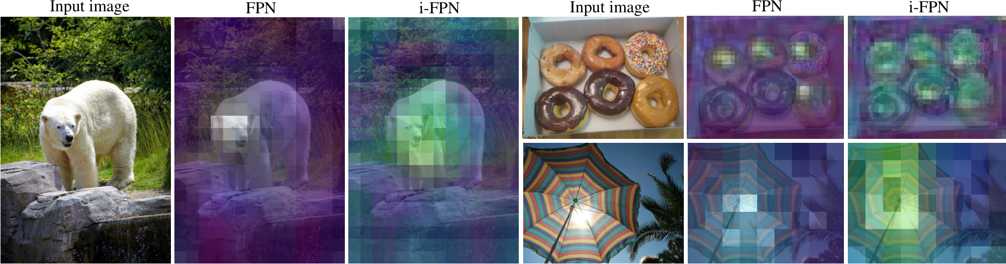
Fig. 5 further shows the comparison between the feature maps obtained using FPN and our i-FPN on several example images from the COCO2017-val dataset. From the visualization results, we can easily find that feature maps produced by FPN are of limited receptive field. In contrast, the feature maps obtained by our i-FPN are of global receptive field and focus on relatively larger regions of interest compared to the feature of the same level from FPN.

Methods	$AP$	$AP_{50}$	$AP_{75}$	$AP_{s}$	$AP_{m}$	$AP_{l}$
RetinaNetLin2017RetinaNet	36.3	56.1	39.1	21.3	40.1	47.9
+ i-FPN	39.7	59.3	42.9	22.9	43.8	52.5
Faster-RCNN fasterrcnn2015	37.7	58.8	41.0	22.0	41.1	49.2
+ i-FPN	40.9	60.4	44.8	25.1	43.8	52.4
FCOS Tian2019FCOS	38.6	57.8	41.7	23.2	42.4	49.7
+ i-FPN	42.1	60.3	45.7	25.7	45.6	54.7
ATSS zhang2020atss	39.3	57.5	42.7	22.9	42.9	51.2
+ i-FPN	43.5	61.0	47.4	26.0	47.5	57.2
AutoAssign zhu2020autoassign	40.5	59.8	43.9	23.1	44.7	52.9
+ i-FPN	43.7	61.4	47.2	25.3	47.4	58.3

Table 1: Performance comparison between FPN lin2017fpn and our i-FPN on some typical one-stage and two-stage object detectors, evaluated on COCO2017-val dataset. ResNet-50 He2016Resnet is employed as the backbone network and 1x training strategy is adopted. For all given object detectors, our i-FPN outperforms original FPN by a large margin.

Refer to caption — Figure 5: Comparison of feature maps obtained using FPN lin2017fpn and i-FPN on example images from the COCO2017-val dataset. The features are extracted from P5-P7 levels and compared with corresponding levels. Features obtained by our i-FPN are of global receptive field compared to the FPN baseline.

4.4 Ablation Study

We perform a thorough ablation study in this section. All the ablation experiments are conducted with ResNet-50 backbone and evaluated on COCO2017-val dataset.

Effect of two different solvers: We firstly explore the effect of using two different solvers, unrolling and Broyden solvers. Tab. 2 shows the performance comparison on AutoAssign, where $G_{\theta}$ adopts the network in Fig. 4(b). The baseline is the AutoAssign without FPN, producing 38.8 box AP. For the unrolling solver, when the weight-sharing block is unrolled with one iteration, the i-FPN achieves 41.2 AP with +2.4% improvement. Increasing the unrolled iteration from 1 to 2 can further improves the box AP by 1.2%. If we continue increasing the iterations, less improvement is achieved. For example, four iterations only improves 0.1% compared to two iterations. On the contrary, our i-FPN with the Broyden solver in bai2019deq directly produces 42.8 AP since it simulates the case of infinite residual-like iterations.

Solver	Iters	$AP$	$AP_{50}$	$AP_{75}$	$AP_{s}$	$AP_{m}$	$AP_{l}$
Unrolling	0	38.8	57.5	42.0	20.5	42.5	52.0
	1	41.2	59.8	44.7	23.2	45.0	53.8
	2	42.4	60.7	45.7	24.4	46.2	55.5
	4	42.5	60.4	46.1	23.5	46.1	56.0
Broyden	$\infty$	42.8	60.8	46.2	24.2	46.4	56.7

Table 2: Analyzing the impact of unrolling and the Broyden solvers. AutoAssign without FPN serves as the baseline detector. Unrolling solver achieves saturated detection performance when the iteration is greater than two. The modified Broyden solver in bai2019deq simulates stacking infinite weight-sharing blocks, which achieves the best performance.

Impact of integrating different components: As mentioned above, the nonlinear transformation $G_{\theta}$ consists of the res-block (RBL) and cross-scale connection (CSC). Here, we conduct experiments on ATSS to analyze the effect of them. As shown in Tab. 3, the standard ATSS without FPN provides a detection AP score of 35.2. Integrating the RBL significantly improves the AP score of 38.0 AP. The large gain in performance shows the impact of RBL on compensating for the non-linearity component of $G_{\theta}$ . Integrating our CSC improves the overall performance from 35.2 to 40.3, which demonstrates the significant importance of cross-scale feature fusion. Further, integrating both the RBL and CSC into the detector significantly boosts the performance from 40.3 to 43.5. Thus, RBL and CSC are two key factors in $G_{\theta}$ : RBL introduces more non-linearity to the implicit function while CSC fuses the features from different levels efficiently.

no FPN	RBL	CSC	$AP$	$AP_{50}$	$AP_{75}$	$AP_{s}$	$AP_{m}$	$AP_{l}$
✓			35.2	51.4	38.0	15.9	37.6	51.2
✓	✓		38.0	54.2	41.4	19.7	40.5	53.2
✓		✓	40.3	57.8	44.1	24.1	44.4	53.4
✓	✓	✓	43.5	61.0	47.4	26.0	47.5	57.2

Table 3: Impact of integrating different components (res-block(RBL) and cross-scale connection(CSC)) in the standard ATSS without FPN. Our final detection framework improves the performance with an overall gain of 8.3% over the ATSS without FPN.

Design of cross-scale connection: Here, we analyze different design choices taken into consideration during the construction of CSC. Tab. 4 reports the detection performance when employing different FPN blocks as the CSC. The baseline is ATSS zhang2020atss without CSC (the second row of Tab. 3). Employing Bi-FPN Tan2020bifpn or NAS-FPN Ghiasi2019nasfpn as the CSC produces a decent performance with the AP score of 41.5 while Dense-FPN provides more improvements by 0.9%. Further, integrating the pyramid convolution Wang2020sepc into Dense-FPN, called Pyramid-FPN, achieves 43.5 AP with 1.1% improvements. Therefore, the hand-crafted or searched basic blocks for explicit FPNs may not be the best choice for the design of CSC in implicit FPN.

Types	$AP$	$AP_{50}$	$AP_{75}$	$AP_{s}$	$AP_{m}$	$AP_{l}$
no CSC	38.0	54.2	41.4	19.7	40.5	53.2
Bi-FPN Tan2020bifpn	41.5	59.2	44.8	24.9	45.1	53.7
NAS-FPN Ghiasi2019nasfpn	41.5	58.9	44.7	24.6	45.2	53.8
Dense-FPN wang2020hrnet	42.4	59.9	45.8	25.7	46.0	55.9
Pyramid-FPN Wang2020sepc	43.5	61.0	47.4	26.0	47.5	57.2

Table 4: Performance comparison between different design choices of cross-scale connection, including Bi-FPN, NAS-FPN Ghiasi2019nasfpn, Dense-FPN wang2020hrnet and Pyramid-FPN Wang2020sepc on ATSS. The Pyramid-FPN produces the best performance.

Effect of Residual-Like Iteration: As mentioned in Sec. 3.2.1, our proposed residual-like iteration(RLIter) is simple and effective compared to the implicit function defined in MDEQ bai2020mdeq. Here, we conduct experiments on RetinaNet Lin2017RetinaNet to verify the effectiveness of our RLIter. We first implement our i-FPN with the implicit function introduced in MDEQ and then simply replace the complex interactive design with our RLIter. As shown in Tab. 5, our RLIter achieves +0.8 mAP improvement compared to the MDEQ approach, which shows the effect of our RLIter benefiting from the simple residual-like design.

Types	$AP$	$AP_{50}$	$AP_{75}$	$AP_{s}$	$AP_{m}$	$AP_{l}$
MDEQ bai2020mdeq	37.2	56.8	40.0	21.3	41.1	49.6
RLIter	38.0	57.3	40.9	21.4	42.0	50.8

Table 5: Performance comparison between our residual-like iteration and the implicit function defined in MDEQ bai2020mdeq. Our residual-like iteration is simple and effective, which improves the performance with an overall gain of 0.8% over the complex interactive design in MDEQ.

Methods	Backbone	Iterations	$AP$	$AP_{50}$	$AP_{75}$	$AP_{s}$	$AP_{m}$	$AP_{l}$
Two-Stage Detector:
R-FCN dai2016rfcn	ResNet-101	280k	29.9	51.9	-	10.8	32.8	45.0
Faster RCNN w FPN lin2017fpn	R-101	100k	36.2	59.1	39.0	18.2	39.0	48.2
Mask R-CNN he2017maskrcnn	X-101	120k	39.8	62.3	43.4	22.1	43.2	51.2
Cascade R-CNN cai2018cascade	R-101	135k	42.8	62.1	46.3	23.7	45.5	55.2
TridentDet li2019tridentnet	R-101-DCN	270k	46.8	67.6	51.5	28.0	51.2	60.5
CBNet liu2020cbnet	Dual-X152	130k	50.0	68.8	54.6	-	-	-
CBNet liu2020cbnet	Triple-X152	130k	50.7	69.8	55.5	-	-	-
Single-Stage Detector:
RetinaNet Lin2017RetinaNet	R-101	180k	39.1	59.1	42.3	21.8	42.7	50.2
CornerNet law2018cornernet	HG-104	500k	40.5	56.5	43.1	19.4	42.7	53.9
CenterNet zhou2019objects	HG-104	750k	42.1	61.1	45.9	24.1	45.5	52.8
RepPoints yang2019reppoints	R-101-DCN	180k	45.0	66.1	49.0	26.6	48.6	57.5
FSAF zhu2019fsaf	X-64x4d-101	180k	42.9	63.8	46.3	26.6	46.2	52.7
FreeAnchor zhang2019freeanchor	X-64x4d-101	180k	44.9	64.4	48.4	26.5	48.0	56.5
FCOS Tian2019FCOS	X-64x4d-101	180k	43.2	62.8	46.6	26.5	46.2	53.3
ATSS zhang2020atss	X-64x4d-101-DCN	180k	47.7	66.5	51.9	29.7	50.8	59.4
BorderDet qiu2020borderdet	X-64x4d-101-DCN	180k	48.0	67.1	52.1	29.4	50.7	60.5
AutoAssign zhu2020autoassign	X-64x4d-101-DCN	180k	48.3	67.4	52.7	29.2	51.0	60.3
PAA kim2020paa	X-64x4d-101-DCN	180k	49.0	67.8	53.3	30.2	52.8	62.2
PAA kim2020paa	X-32x8d-152-DCN	180k	50.8	69.7	55.1	31.4	54.7	65.2
Our i-FPN w/ ATSS:
ATSS w/ i-FPN	X-64x4d-101-DCN	180k	49.1	67.3	53.1	32.0	52.9	63.5
ATSS w/ i-FPN	X-32x8d-152-DCN	180k	49.9	68.4	54.0	32.0	53.6	64.2
Our i-FPN w/ Autoassign:
AutoAssign w/ i-FPN	X-64x4d-101-DCN	180k	50.6	69.4	54.9	31.2	53.3	63.7
AutoAssign w/ i-FPN	X-32x8d-152-DCN	180k	52.2	70.9	56.5	32.5	55.1	65.8

Table 6: Performance comparison with state-of-the-art methods on MS COCO test-dev set. All the results are obtained by single-model and single-scale testing. Bold text means the best performance. AutoAssign equipped with our proposed i-FPN outperforms both two-stage and single-stage object detectors.’R’: ResNet. ’X’: ResNeXt. HG: Hourglass.

4.5 State-of-the-art Comparison

In this section, we compare our approach to state-of-the-art object detectors on the COCO2017 test-dev dataset. We follow the training strategies from previous works Tian2019FCOS; zhang2020atss, where the shorter side of images is randomly resized to a scale between 640 to 800. In addition, we adopt the 2x training schedule, where the learning rate is reduced by 10x at 120 $k$ and 160 $k$ iterations with a overall 180 $k$ iterations. Other settings are the same as those mentioned in Sec. 4.2.

As shown in Tab. 6, we report the performance of our i-FPN equipped with anchor-free detectors, ATSS zhang2020atss and AutoAssign zhu2020autoassign. Note that all the results are obtained by single-model and single-scale testing. The strong baseline, ATSS zhang2020atss with ResNeXt-64x4d-101-DCN backbone, provides the detection performance with AP score of 47.7. Equipped with our i-FPN, ATSS achieves 49.1 AP with 1.4% improvement, which is better than those detectors with the same backbones. The overall AP can be further improved to 49.9 by introducing larger backbone, ResNeXt-32x8d-152-DCN. Similar conclusion can be drawn from AutoAssign. Compared to the strong baseline AutoAssign with ResNeXt-64x4d-101-DCN backbone, i-FPN can boost the performance from 48.3 to 50.6, with 2.3% AP improvements. The 50.6 AP result surpasses all anchor-free and anchor-based detectors with the same backbone and is better than the state-of-the-art approach, PAA kim2020paa with 1.6%. For further comparison with PAA, we also conduct experiments with the ResNeXt-32x8d-152-DCN backbone. AutoAssign with our i-FPN achieves 52.2 AP on a single model with single-scale testing, outperforming the PAA by 1.4% under the same condition. Also, our best model with 52.2 AP is even better than the two-stage detectors, such as CBNet liu2020cbnet and TridentDet li2019tridentnet.

5 Limitation and Future Work

Though our proposed i-FPN significantly boosts the performance of object detectors, the new design for FPN also comes with some drawbacks. The employment of unrolling solver still results in large memory burden with the increase of iterations though it achieves weight-sharing of all unrolled blocks. For the Broyden solver, it takes another 15 Broyden iterations to obtain the equilibrium feature pyramid for each iteration of object detector. Therefore, it takes almost 6x time for the detector learning compared to the detectors with explicit FPN even though it only requires memory of a single block. During testing stage, we find that same detection result can be obtained when the Broyden iterations reduce to 7. Developing an efficient solver is one of important future topics.

References

(1) Luis B Almeida. A learning rule for asynchronous perceptrons with feedback in a combinatorial environment. In Artificial neural networks, 1990.
(2) Shaojie Bai, J. Zico Kolter, and Vladlen Koltun. Deep equilibrium models. In NeurlPS, 2019.
(3) Shaojie Bai, J. Zico Kolter, and Vladlen Koltun. Trellis networks for sequence modeling. In ICLR, 2019.
(4) Shaojie Bai, Vladlen Koltun, and J. Zico Kolter. Multiscale deep equilibrium models. arXiv preprint arXiv:2006.08656, 2020.
(5) Alexey Bochkovskiy, Chien-Yao Wang, and Hong-Yuan Mark Liao. Yolov4: Optimal speed and accuracy of object detection. arXiv preprint arXiv:2004.10934, 2020.
(6) Charles G Broyden. A class of methods for solving nonlinear simultaneous equations. Mathematics of computation, 1965.
(7) Zhaowei Cai and Nuno Vasconcelos. Cascade r-cnn: Delving into high quality object detection. In CVPR, 2018.
(8) Nicolas Carion, Francisco Massa, Gabriel Synnaeve, Nicolas Usunier, Alexander Kirillov, and Sergey Zagoruyko. End-to-end object detection with transformers. In ECCV, 2020.
(9) Ricky TQ Chen, Yulia Rubanova, Jesse Bettencourt, and David K Duvenaud. Neural ordinary differential equations. In NeurlPS, 2018.
(10) Raj Dabre and Atsushi Fujita. Recurrent stacking of layers for compact neural machine translation models. In AAAI, 2019.
(11) Jifeng Dai, Yi Li, Kaiming He, and Jian Sun. R-fcn: Object detection via region-based fully convolutional networks. In Advances in neural information processing systems, 2016.
(12) Mostafa Dehghani, Stephan Gouws, Oriol Vinyals, Jakob Uszkoreit, and Lukasz Kaiser. Universal transformers. In ICLR, 2018.
(13) Kaiwen Duan, Song Bai, Lingxi Xie, Honggang Qi, Qingming Huang, and Qi Tian. Centernet: Keypoint triplets for object detection. In CVPR, 2019.
(14) Laurent El Ghaoui, Fangda Gu, Bertrand Travacca, and Armin Askari. Implicit deep learning. arXiv preprint arXiv:1908.06315, 2019.
(15) Yarin Gal and Zoubin Ghahramani. A theoretically grounded application of dropout in recurrent neural networks. In NeurlPS, 2016.
(16) Golnaz Ghiasi, Tsung-Yi Lin, Ruoming Pang, and Quoc V. Le. Nas-fpn: Learning scalable feature pyramid architecture for object detection. In CVPR, 2019.
(17) Eldad Haber and Lars Ruthotto. Stable architectures for deep neural networks. Inverse Problems, 2017.
(18) Kaiming He, Gorgia Gkioxari, Piotr Dollár, and Ross Girshick. Mask r-cnn. In ICCV, 2017.
(19) Kaiming He, Xiangyu Zhang, Shaoqing Ren, and Jian Sun. Deep residual learning for image recognition. In CVPR, 2016.
(20) Kaiming He, Xiangyu Zhang, Shaoqing Ren, and Jian Sun. Identity mappings in deep residual networks. In ECCV, 2016.
(21) Kang Kim and Hee Seok Lee. Probabilistic anchor assignment with iou prediction for object detection. In ECCV, 2020.
(22) Tao Kong, Fuchun Sun, Huaping Liu, Yuning Jiang, Lei Li, and Jianbo Shi. Foveabox: Beyound anchor-based object detection. TIP, 2020.
(23) Hei Law and Jia Deng. Cornernet: Detecting objects as paired keypoints. In ECCV, 2018.
(24) Yanghao Li, Yuntao Chen, Naiyan Wang, and Zhaoxiang Zhang. Scale-aware trident networks for object detection. In ICCV, 2019.
(25) Renjie Liao, Yuwen Xiong, Ethan Fetaya, Lisa Zhang, KiJung Yoon, Xaq Pitkow, Raquel Urtasun, and Richard Zemel. Reviving and improving recurrent back-propagation. In ICML, 2018.
(26) Tsung-Yi Lin, Piotr Dollar, Ross Girshick, Kaiming He, Bharath Hariharan, and Serge Belongie. Feature pyramid networks for object detection. In CVPR, 2017.
(27) Tsung-Yi Lin, Priya Goyal, Ross Girshick, Kaiming He, and Piotr Dollár. Focal loss for dense object detection. In ICCV, 2017.
(28) Tsung-Yi Lin, Michael Maire, Serge Belongie, James Hays, Pietro Perona, Deva Ramanan, Piotr Dollár, and C. Lawrence Zitnick. Microsoft coco: Common objects in context. In ECCV, 2014.
(29) Songtao Liu and Di Huang. Receptive field block net for accurate and fast object detection. In ECCV, 2018.
(30) Shu Liu, Lu Qi, Haifang Qin, Jianping Shi, and Jiaya Jia. Path aggregation network for instance segmentation. In CVPR, 2018.
(31) Wei Liu, Dragomir Anguelov, Dumitru Erhan, Christian Szegedy, Scott Reed, Cheng-Yang Fu, and Alexander C. Berg. SSD: Single shot multibox detector. In ECCV, 2016.
(32) Yudong Liu, Yongtao Wang, Siwei Wang, TingTing Liang, Qijie Zhao, Zhi Tang, and Haibin Ling. Cbnet: A novel composite backbone network architecture for object detection. In AAAI, 2020.
(33) Fernando J Pineda. Generalization of back propagation to recurrent and higher order neural networks. In NeurlPS, 1988.
(34) Siyuan Qiao, Liang-Chieh Chen, and Alan Yuille. Detectors: Detecting objects with recursive feature pyramid and switchable atrous convolution. arXiv preprint arXiv:2006.02334, 2020.
(35) Han Qiu, Yuchen Ma, Zeming Li, Songtao Liu, and Jian Sun. Borderdet: Border feature for dense object detection. In ECCV, 2020.
(36) Joseph Redmon, Santosh Divvala, Ross Girshick, and Ali Farhadi. You only look once: Unified, real-time object detection. In CVPR, 2016.
(37) Shaoqing Ren, Kaiming He, Ross Girshick, and Jian Sun. Faster R-CNN: Towards real-time object detection with region proposal networks. In NeurlPS, 2015.
(38) Olga Russakovsky, Jia Deng, Hao Su, Jonathan Krause, Sanjeev Satheesh, Sean Ma, Zhiheng Huang, Andrej Karpathy, Aditya Khosla, Michael Bernstein, Alexander C. Berg, and Li Fei-Fei. Imagenet large scale visual recognition challenge. In IJCV, 2015.
(39) Tim Salimans and Durk P. Kingma. Weight normalization: A simple reparameterization to accelerate training of deep neural networks. In NeurlPS, 2016.
(40) Patrice Y Simard, Mary B Ottaway, and Dana H Ballard. Fixed point analysis for recurrent networks. In NeurlPS, 1989.
(41) Karen Simonyan and Andrew Zisserman. Very deep convolutional networks for large-scale image recognition. In NIPS, 2014.
(42) Bharat Singh and Larry S Davis. An analysis of scale invariance in object detection snip. In CVPR, 2018.
(43) Mingxing Tan and Quoc Le. Efficientnet: Rethinking model scaling for convolutional neural networks. In ICML, 2019.
(44) Mingxing Tan, Ruoming Pang, and Quoc V. Le. Efficientdet: Scalable and efficient object detection. In CVPR, 2020.
(45) Zachary Teed and Jia Deng. Raft: Recurrent all-pairs field transforms for optical flow. In ECCV, 2020.
(46) Zhi Tian, Chunhua Shen, Hao Chen, and Tong He. Fcos: Fully convolutional one-stage object detection. In ICCV, 2019.
(47) Jingdong Wang, Ke Sun, Tianheng Cheng, Borui Jiang, Chaorui Deng, Yang Zhao, Dong Liu, Yadong Mu, Mingkui Tan, Xinggang Wang, et al. Deep high-resolution representation learning for visual recognition. TPAMI, 2020.
(48) Xinjiang Wang, Shilong Zhang, Zhuoran Yu, Litong Feng, and Wayne Zhang. Scale-equalizing pyramid convolution for object detection. In CVPR, 2020.
(49) Yuxin Wu and Kaiming He. Group normalization. In ECCV, 2018.
(50) Ze Yang, Shaohui Liu, Han Hu, Liwei Wang, and Stephen Lin. Reppoints: Point set representation for object detection. In ICCV, 2019.
(51) Shifeng Zhang, Cheng Chi, Yongqiang Yao, Zhen Lei, and Stan Z Li. Bridging the gap between anchor-based and anchor-free detection via adaptive training sample selection. In CVPR, 2020.
(52) Xiaosong Zhang, Fang Wan, Chang Liu, Rongrong Ji, and Qixiang Ye. Freeanchor: Learning to match anchors for visual object detection. In NeurlPS, 2019.
(53) Xingyi Zhou, Dequan Wang, and Philipp Krähenbühl. Objects as points. arXiv preprint arXiv:1904.07850, 2019.
(54) Xingyi Zhou, Jiacheng Zhuo, and Philipp Krahenbuhl. Bottom-up object detection by grouping extreme and center points. In CVPR, 2019.
(55) Benjin Zhu, Jianfeng Wang, Zhengkai Jiang, Fuhang Zong, Songtao Liu, Zeming Li, and Jian Sun. Autoassign: Differentiable label assignment for dense object detection. arXiv preprint arXiv:2007.03496, 2020.
(56) Chenchen Zhu, Yihui He, and Marios Savvides. Feature selective anchor-free module for single-shot object detection. In CVPR, 2019.