Scalarization-like mechanism through spacetime anisotropic scaling symmetry

A remarkable characteristic of the black hole solutions in Einstein’s gravity is the fact that, despite the complexity involved, each configuration is defined by a reduced set of parameters. For asymptotically flat spacetimes, Israel initiated in the pursue of the so-called uniqueness theorems five decades ago [1]. In short, they state that the most general stationary and axisymmetric electrovacuum black holes with a positive mass reduce to the Kerr-Newman class [2]. In the same line the emergence of no-hair conjectures, first hinted by Ruffini and Wheeler [3], takes care of sorting out the type of matter fields allowed to exist around regular black holes. As a result, increasing the number of effectively independent parameters is restricted to very specific circumstances. In more detail, the classical no-hair theorems later formalized by Bekenstein [4] provide arguments — independent of the gravitational dynamics — asserting that black holes are characterized only by conserved charges subject to Gauss-like laws such as the mass, angular momentum and electromagnetic charge. Coupling a scalar field (either massless or massive), a Proca field or a massive spin-2 field around a stationary black hole is shown to fail. Further refinement on the arguments [5] and extensions to explore different asymptotes and matter self-interactions appeared over the years, see [6] for a few examples. However, the reach and efficacy of no hair theorems are heavily dependent on the assumptions under which forged. Therefore, alongside the derivation of such conjectures, many counter examples of black holes or compact objects supporting nongauge fields in their exterior have been reported, the so-called hairy configurations.

When a field not associated to a conservation law is regular everywhere in the exterior of the black hole, it is called a hair. The first and most celebrated candidates to be hairy configurations were found not much after the no-hair conjectures were introduced. In [7], a conformal coupling between a scalar field and the curvature proved an effective mechanism to evade the conjecture’s axioms. Similarly, in [8] and later in [9] a family of so-called colored back holes were reported. In these cases, the spherical solutions are supported by a $\displaystyle SU(2)$ Yang-Mills field. It was afterwards shown that both a priori appealing solutions suffer from undesirable properties such as instabilities under linear perturbations, [10] and [11] respectively. Further, an ADM mass formula for the solitons of the Einstein-Yang-Mills system in terms of black hole horizon properties was obtained by using the isolated horizon formalism [12]. These models for colored black holes settled the basis for general strategies to overcome the no-hair impossibilities previously established. This fact, together with new theoretical frameworks, gave rise to a very active search for genuinely hairy black holes. For a nice review on the recent progress, we refer the reader to [13].

Closely related to the hairy scenario, a more recent phenomenon has gained plenty of attention from the community: spontaneous scalarization. Originally discussed in the context of neutron stars [14, 15], it was noted that a tensor-scalar configuration could become nontrivial for a specific range of parameters — the total mass in that particular case. Furthermore, the finite scalar configuration turned to be preferable, energetically speaking, as compared to the scalar-free case. A detailed analysis and review can be found in [16]. It was spotted in the original works [14] that spontaneous scalarization can leave the weak gravity limit untouched and be fitted to manifests itself only in strong gravity processes. This means of course that the standard solar system tests would be blind to it. Actually, the machinery is ready to compare and probe the possible scalarized nature of black holes. For instance, forthcoming gravitational wave interferometry — the LISA observatory in particular — seems capable of shedding some light on the issue [17]. In a similar fashion, the new achievements in black hole shadow imaging can, in principle, provide evidence on possible scalar imprints [18].

Spontaneously scalarized spacetimes are field configurations that are smoothly connected with a scalar-free solution to a given theory. A generic characteristic of such setups is that over the scalar-free background, the propagation of the scalar field would exhibit a tachyonic mode. The mechanisms driving spontaneous scalarization come from an effective nonminimal coupling between the scalar field and either additional (matter) fields, the geometry or both. Such a setup is well captured by the action,

$\displaystyle\displaystyle S[g_{\mu\nu},\phi,\Psi]=\int{d^{D}x\sqrt{-g}\left[\frac{R-2\lambda}{2\kappa}+\mathcal{L}_{\text{SF}}\left(g_{\mu\nu},\phi,\nabla_{\mu}\phi\right)+h(\phi)\mathcal{I}\left(g_{\mu\nu},\Psi,R^{\alpha}_{\beta\mu\nu}\right)\right]},$

(1.1)

defined over $\displaystyle D$ spacetime dimensions in the presence of a cosmological constant $\displaystyle\lambda$ and where $\displaystyle\kappa$ is the Einstein’s gravitational constant. The function $\displaystyle\mathcal{I}$ can depend on a standard Lagrangian for the fields $\displaystyle\Psi$ and the curvature, and the arbitrary function $\displaystyle h$ measures the nonminimal coupling between the scalar field and it. Notice that the dynamics of the scalar can be as generic as desired and it is given by the Lagrangian $\displaystyle\mathcal{L}_{\text{SF}}$. During the past two decades numerous examples fitting in (1.1) have been reported. To mention a few of the most notorious, when $\displaystyle\mathcal{I}$ is taken as the Gauss-Bonnet term, static spherical black holes have been shown to scalarize for various nonminimal coupling functions [19] as well as rotating configuration[20]. More related to this work is the case when $\displaystyle\mathcal{I}$ is a function of the Maxwell term, thus exhibiting scalarization when the scalar field is nonminimally coupled to a gauge field [21, 22, 23]. As a particular application, in [24] it was argued that spontaneous scalarization in compact objects (polytropic fluids) is accompanied by a spontaneous violation of the weak energy condition. However, in [25] it was further shown that the negativeness of such energy densities is not generic of scalar-tensor theories of gravity by using realistic models of dense matter. Further examples and a review on the topic can be found in [26] and [27] respectively.

Very recently, in [28] the idea of achieving spontaneous scalarization through breaking scale invariance was worked out. There, quantum corrections to the Einstein-Maxwell theory are added in the form of a quartic term in the field strength, breaking thus the natural Weyl invariance of Maxwell’s theory. In this work, we find that a similar effect — yet not identical, as later made precise — can be achieved by breaking the spacetime isotropy, that is, the scaling symmetry between the timelike and spatial directions. Backgrounds with this property are called anisotropic, and the most iconic example is the Lifshitz spacetime which we proceed to describe.

A good motivation to delve into anisotropic spaces is the cornerstone problem of the quantization of gravity. There are various problems arising in the UV regimes of gravitational theories. Among them, the dimensions carried by the coupling (Newton’s) constant $\displaystyle[G_{D=4}]\sim L^{2}$ spoil its renormalizability [29]. This can be corrected to the case of dimensionless coupling at the cost of introducing an scaling asymmetry between time and space, as explored in Horava-like gravities [30]. The natural setup for it to take place is a Lifshitz spacetime. Originally introduced in [31], it is understood as a gravitational dual to non-Lorentz invariant quantum field theories. Therein, the deviation from spacetime isotropy is measured by the so-called critical dynamical exponent $\displaystyle z$. The metric of a Lifshitz spacetime takes the form

$\displaystyle\displaystyle g_{\text{Lifshitz}}=-\left(\dfrac{r}{l}\right)^{2z}dt^{2}+\dfrac{dr^{2}}{\left(\dfrac{r}{l}\right)^{2}}+\left(\dfrac{r}{l}\right)^{2}\sum^{D-2}_{k=1}dx^{2}_{k}.$

(1.2)

In these coordinates, it turns out to be invariant under the anisotropic scaling transformations $\displaystyle D_{z},$

$$t\mapsto\lambda^{z}t,\qquad\,\quad r\mapsto\dfrac{r}{\lambda},\qquad\,\quad x_{k}\mapsto\lambda x_{k},$$

(1.3)

as well as under space and time translations and spatial rotations:

	$\displaystyle\displaystyle H:$		$\displaystyle\displaystyle\,\,\,t\longrightarrow\,\,\,t^{\prime}=t+a;$
	$\displaystyle\displaystyle P^{i}:$		$\displaystyle\displaystyle x^{i}\longrightarrow x^{{}^{\prime}i}=x^{i}+a^{i};$		(1.4)
	$\displaystyle\displaystyle L^{ij}:$		$\displaystyle\displaystyle x^{i}\longrightarrow x^{{}^{\prime}i}=L^{i}_{j}x^{j}.$

Lifshitz spacetimes are anisotropic generalizations of anti-de Sitter (AdS) that also have constant negative curvature and share many of the geometrical and physical properties. For instance, the existence of a boundary and the corresponding confining character as well as a Breitenlohner-Freedman (BF) bound for the energy — or mass spectrum — of fields dynamically coupled to gravity. We shall consider the parameter $\displaystyle z\geq 1$ to be continuous for the purposes of our work. Inviting to us, the idea that Lorentz invariance is the low energy effect of a more fundamental anisotropic theory has been entertained [32]. In the same line of thought, we can consider that the anisotropic parameter $\displaystyle z$ that encodes the measure of Lorentz symmetry violation, achieves the relativistic limit when $\displaystyle z=1$, recovering the isotropy between space and time scaling transformations.

Naturally, while breaking the Lorentzian symmetry, Lifshitz backgrounds are not expected solutions to standard gravitational theories. Therefore, the occurrence of nontrivial gravitational phenomena such as black holes requires either a modification on the dynamics or an enhancement through additional matter fields. For example, the first asymptotically Lifshitz back holes were reported in [33, 34, 35], one in the context of Einstein-Maxwell-Dilaton theory and the latter in gravities with quadratic corrections.

In the present manuscript, we show how the spacetime anisotropy can be supplemented by a more generic matter arrangement than the Maxwell-Dilaton case. By assuming a simple static Lifshitz ansatz, we find a novel exact charged black hole configuration. A nontrivial scalar field configuration manifests itself as one deviates from the isotropic case; i.e., $\displaystyle z>1$. As we will explore in detail, these solutions are thermodynamically favorable under the existence of the scalar field. In this sense, we argue on favor of a scalarization phenomenom akin to the spontaneous scalarization reviewed above.

Organization of the paper.   In Sec. 2 we introduce the theoretical framework describing the nonminimal coupling between the scalar and a Maxwell field. For it, we find a four-dimensional solution shown to accommodate an event horizon in Sec. 2.2. Later, in Sec. 3 we extend the result to a higher dimensional black hole and prove in Sec. 3.3 that it fulfils the scalarization conditions. The conserved charges and corresponding thermodynamics are provided in Sec. 4. With these results, we finally discuss thermodynamical arguments favoring the scalarized (anisotropic) configuration in Sec. 5. We conclude with some important remarks and a discussion in Sec. 6.

The existence of scalarized solutions conceded by an adequate source term in the scalar field equation. This source originates from the nonminimal coupling between the scalar mode and either additional matter or the curvature, as depicted in (1.1). For our purposes, we will track down the first possibility. In particular, we will introduce a vector field $\displaystyle A_{\mu}$ such that $\displaystyle\mathcal{I}$ is chosen as the Maxwell’s kinetic term. Being the nonminimal coupling function arbitrary, our starting point results in a generalization of the standard Einstein-Maxwell-Dilaton theory in four spacetime dimensions¹¹ 1 Pioneer research on black hole solutions to Dilaton gravity is reported in [36, 37]. Also relevant in this context is the Lifshitz solution in [33, 34, 35]. . Namely, the action of our framework reads

$\displaystyle\displaystyle S\left[g_{\mu\nu},A_{\mu},\phi\right]=\int{d^{4}x\sqrt{-g}\Big(\frac{R-2\lambda}{2\kappa}-\frac{1}{2}\partial_{\mu}\phi\partial^{\mu}\phi-\frac{h(\phi)}{4}F_{\mu\nu}F^{\mu\nu}\Big)},$

(2.1)

where $\displaystyle F_{\mu\nu}:=\nabla_{\mu}A_{\nu}-\nabla_{\nu}A_{\mu}$ is the field strength and we recall that $\displaystyle h(\phi)$ is a nonminimal coupling function. The coupling does not carry derivatives of the scalar so that the number of degrees of freedom is trivially preserved. Following the standard notation, $\displaystyle R$ is the scalar curvature, $\displaystyle\lambda$ is a cosmological constant, and $\displaystyle\kappa$ is the Einstein’s gravitational constant. Notice that in order to preserve an smooth decoupling limit between the scalar and the vector, the minimal requirement is that $\displaystyle h(\phi_{0})=\text{const}$ for a trivial (ground) value $\displaystyle\phi_{0}$ of the scalar field. When $\displaystyle h(\phi)=e^{-\alpha\phi}$, with $\displaystyle\alpha$ and arbitrary constant, the Einstein-Maxwell-Dilaton theory is recovered.

The field equations derived from (2.1) through the action principle read

$\displaystyle\displaystyle\mathcal{E}_{\mu\nu}:=R_{\mu\nu}-\frac{1}{2}Rg_{\mu\nu}+\lambda g_{\mu\nu}-\kappa T_{\mu\nu}=0,\qquad\,\,\nabla_{\nu}\left(hF^{\mu\nu}\right)=0,\qquad\,\,\Box\phi-\frac{1}{4}\frac{dh}{d\phi}F_{\mu\nu}F^{\mu\nu}=0,$

(2.2)

where the total energy-momentum tensor contains information from both matter fields and it is conformed by

$\displaystyle\displaystyle T_{\mu\nu}=T^{\phi}_{\mu\nu}+hT^{A}_{\mu\nu},\qquad\qquad\nabla_{\mu}T^{\mu\nu}=0,$

(2.3)

with $\displaystyle T^{\phi}_{\mu\nu}$ the free scalar field energy-momentum tensor and $\displaystyle T^{A}_{\mu\nu}$ the one for the Maxwell field, i.e,

$\displaystyle\displaystyle T^{\phi}_{\mu\nu}=\partial_{\mu}\phi\partial_{\nu}\phi-\frac{1}{2}(\partial_{\alpha}\phi\partial^{\alpha}\phi)g_{\mu\nu},\qquad\quad\ T^{A}_{\mu\nu}=F_{\mu\alpha}{F_{\nu}}^{\alpha}-\frac{1}{4}F_{\alpha\beta}F^{\alpha\beta}g_{\mu\nu}.$

(2.4)

We point out that the first scrutiny of this system in the context of scalarization was in [21]. There, it was first observed that the nonminimal coupling between the scalar field and the Maxwell invariant can trigger the spontaneous scalarization of the asymptotically flat Reissner-Nordström black hole. In this section, we will follow a similar approach by exploring solutions with the difference that we will build upon an asymptotically Lifshitz background.

The action in Eq. (2.1) can be straightforwardly generalized to an arbitrary dimension,

$\displaystyle\displaystyle S[g,A,\phi]=\int{d^{D}x\sqrt{-g}\Big(\frac{R-2\lambda}{2\kappa}-\frac{1}{2}\partial_{\mu}\phi\partial^{\mu}\phi-\frac{h(\phi)}{4}F_{\mu\nu}F^{\mu\nu}\Big)}.$

(3.1)

On its own merit, higher dimensional gravities are worth attention. Yet, a more interesting motivation is their connection with the gauge/gravity duality connecting a bulk $\displaystyle D$ dimensional theory with a $\displaystyle D-1$ boundary conformal theory. The canonical example is the celebrated AdS/CFT correspondence [41], where the gravitational dual resides in a type IIB string theory over $\displaystyle AdS_{5}\times S^{5}$. From the Lifshitz anisotropic side, the breaking of the Lorentz invariance allows one to relate through duality nonrelativistic quantum systems as those pertinent for condensed matter physics [42]. Therefore, higher-dimensional Lifshitz gravities open a window that extends the applicability of the gauge/gravity duality to a wide plethora of quantum systems under the so-called gravity/condensed matter theory correspondence [43]. From now on we will focus only in the gravitational side and expect to push ahead the understanding of the dual quantum field theory side.

The thermodynamics of black holes with different to flat asymptotics has been a major field of investigation. For our concrete case of interests, a Lifshitz asymptote, the study of the thermodynamics was initiated in[51] and vastly developed later [52]. In these works, it is determined how the critical dynamical exponent plays a major role in the form of the conserved charges. As a consequence, the first law and other relevant thermodynamical properties get modified by the spacetime anisotropy.

We proceed to compute the quantities characterizing the horizon. The Hawking temperature, defined in terms of the surface gravity $\displaystyle\tilde{\kappa}$, is given by means of the relation

$$T_{H}\equiv\frac{\tilde{\kappa}}{2\pi},\qquad\text{with}\qquad\tilde{\kappa}^{2}=-\frac{1}{2}\left(\nabla_{\mu}\chi_{\nu}\right)\left(\nabla^{\mu}\chi^{\nu}\right),$$

(4.1)

where $\displaystyle\chi=\chi^{\mu}\partial_{\mu}=\partial_{t}$ is the generator of the event horizon. Accordingly, the Hawking temperature associated with the $\displaystyle D$-dimensional configuration (3.1) reads

$$T_{H}=\frac{1}{4\pi}\frac{(z+D-2)r_{H}^{z}-b(z+D-4)r_{H}^{-(z+2D-6)}}{\ell^{z+1}},$$

(4.2)

whereas the Wald entropy results proportional to the event horizon area $\displaystyle\mathcal{A}$ and takes the form,

$$\mathcal{S}\equiv\frac{\mathcal{A}}{4G_{D}}=\dfrac{V_{D-2}}{4G_{D}}\left(\dfrac{r_{H}}{\ell}\right)^{D-2},$$

(4.3)

where $\displaystyle G_{D}=\kappa/8\pi$ is the $\displaystyle D$-dimensional gravitational constant and $\displaystyle V_{D-2}$ represents the Euclidean volume of the spatial sector.
The electric charge can be computed through a Gaussian integral over a spatial hypersurface $\displaystyle\Sigma$ at asymptotic infinity

$$Q_{\text{e}}=\int_{\Sigma}d^{D-2}x\sqrt{|\gamma|}n^{\mu}u^{\nu}h(\phi)F_{\mu\nu}=QV_{D-2},$$

(4.4)

where $\displaystyle\gamma$ is the induced metric on $\displaystyle\Sigma$, with $\displaystyle u$ and $\displaystyle n$ its timelike and spacelike normal unit vectors

$$u^{\mu}=\dfrac{1}{\sqrt{f(r)}}\left(\dfrac{l}{r}\right)^{z},\qquad\quad n^{\mu}=\sqrt{f(r)}\,\dfrac{r}{l}.$$

(4.5)

The electrostatic potential associated with the Maxwell field is defined as

$$\Phi_{e}:=A(r_{H})=\dfrac{1}{4lQ\kappa}\left[(z-1)\left(\dfrac{r_{H}}{l}\right)^{z+D-2}-(D-2)\dfrac{b}{l^{2(z+D-3)}}\left(\dfrac{r_{H}}{l}\right)^{4-z-D}\right].$$

(4.6)

Next, in order to compute the total energy carried by our black hole configuration we exploit the so-called generalized ADT quasilocal method, foremost introduced in [53]. This method has been implemented and proved to be well suited in the construction of conserved charges in higher order gravity theories (see, for instance, [54, 55, 56, 57]), as well as Einstein-Maxwell-Dilaton theories [58]. In this method, the conserved charge corresponding to a killing vector field $\displaystyle\xi$ is given by

$$\mathcal{Q}(\xi)=\int d^{D-2}x_{\mu\nu}\left(\Delta K^{\mu\nu}(\xi)-2\xi^{[\mu}\int_{0}^{1}ds\Theta^{\nu]}(\xi,s)\right),$$

(4.7)

with $\displaystyle d^{D-2}x_{\mu\nu}:=\frac{\epsilon_{\mu\nu\mu_{1}\mu_{2}\ldots\mu_{D-2}}}{2(D-2)!}dx^{\mu_{1}}\wedge\ldots\wedge dx^{\mu_{D-2}}$. Here $\displaystyle\epsilon_{\mu\nu\mu_{1}\mu_{2}\ldots\mu_{D-2}}$ corresponds to the totally antisymmetric Levi-Civita symbol in $\displaystyle D-2$ dimensions. On the other hand, $\displaystyle s$ stands for a parameter allowing an interpolation of the black hole configuration between the solution of interest ($\displaystyle s=1$) and the asymptotic one ($\displaystyle s=0$). Furthermore, $\displaystyle\Delta K^{\mu\nu}(\xi)=K^{\mu\nu}_{s=1}(\xi)-K^{\mu\nu}_{s=0}(\xi)$ stands for the total difference of the Noether potentials between the two end points of the path, $\displaystyle s=[0,1]$. Finally, $\displaystyle\Theta^{\nu}$ is the surface term usually disregarded during the variation of the action but that has an instrumental role in the construction of the off shell Noether current [53]. In general, it has a nontrivial contribution to the quasilocal global charges and it is particularly important in our calculations of the mass. The Noether potential and the surface terms associated to our model are found to be

	$\displaystyle\displaystyle K^{\mu\nu}(\xi)$	$\displaystyle\displaystyle=2\sqrt{-g}\left[\frac{\nabla^{[\mu}\xi^{\nu]}}{2\kappa}-\frac{1}{2}\frac{\partial\mathcal{L}}{\partial(\partial_{\mu}A_{\nu})}\xi^{\sigma}A_{\sigma}\right],$		(4.8)
	$\displaystyle\displaystyle\Theta^{\mu}(\delta g,\delta\phi,\delta A)$	$\displaystyle\displaystyle=2\sqrt{-g}\left(\frac{g^{\alpha[\mu}\nabla^{\beta]}\delta g_{\alpha\beta}}{2\kappa}+\frac{1}{2}\frac{\partial\mathcal{L}}{\partial(\partial_{\mu}A_{\nu})}\delta A_{\nu}+\frac{1}{2}\frac{\partial\mathcal{L}}{\partial(\partial_{\mu}\phi)}\delta\phi\right).$		(4.9)

To compute the mass according to (4.7), the timelike Killing vector takes the form $\displaystyle\eta=\eta^{\mu}\partial_{\mu}=\partial_{t}$. This expression, together with the nontrivial contributions coming from (4.8) and (4.9), lead subsequently to

$$\mathcal{M}=\frac{V_{D-2}}{2\kappa\ell}(D-2)\left[1+b\,r_{H}^{-2(z+D-3)}\right]\left(\dfrac{r_{H}}{\ell}\right)^{z+D-2}.$$

(4.10)

By making use of the expressions (4.10), (4.2), (4.3), (4.6), and (4.4), it is easy to check that the first law of thermodynamics is satisfied

$$d\mathcal{M}=T_{H}d\mathcal{S}+\Phi_{e}dQ_{e},$$

(4.11)

where there is no effective contribution from the electric work since $\displaystyle Q_{e}$ is independent of $\displaystyle r_{H}$.²² 2 The Gibbs free energy ($\displaystyle\mathcal{G}$) representation of the first law $\displaystyle d\mathcal{G}=Q_{e}d\Phi_{e}-SdT_{H}$, indeed has an explicit electrical contribution. However, it will be relevant for the Smarr-like formula below. The following integral relation between the thermodynamical quantities holds

$$\mathcal{M}-\left(\dfrac{D-2}{z+D-2}\right)T\mathcal{S}=b\,\dfrac{(D-2)(z+D-3)}{(z+D-2)}\dfrac{V_{D-2}}{\kappa l^{z+D-1}}r_{H}^{-(z+D-4)},$$

(4.12)

which reduces to the previously reported [33, 58] when the parameter $\displaystyle b$ goes to zero. The last expression can be translated to a Smarr-like formula,

$$\mathcal{M}=\dfrac{D-2}{D-z}\left(T_{H}S-4Q_{\text{e}}\Phi_{\text{e}}\right).$$

(4.13)

One must observe that there is no contribution of a scalar charge neither in the first law or the Smarr formula, contrary to similar reported results [44]. This is consequence of the nondecaying character of our field, but a more subtle analysis is needed since we are not in an asymptotically flat case.

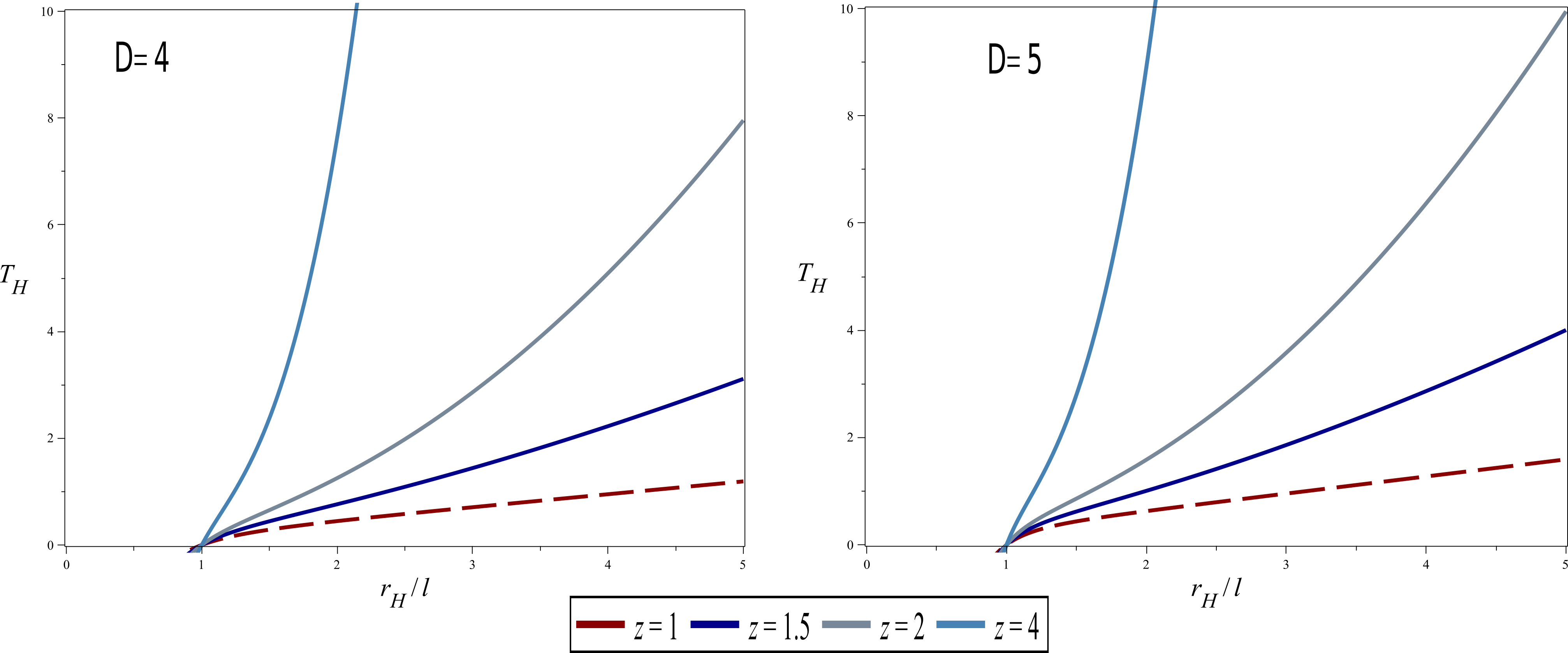
Since the horizon radius is chosen as an independent and arbitrary parameter, there are no further reality or positivity restrictions to impose. Thus, the charge $\displaystyle Q_{\text{e}}$, mass $\displaystyle\mathcal{M}$ or the coupling $\displaystyle b$ need not obey further restrictions. Nonetheless, thermodynamical quantities still need to satisfy reasonable conditions such as a positive temperature and an always increasing entropy. In terms of $\displaystyle r_{H}$, the later condition, the second law is well posed according to (4.3). On the other hand, demanding a non-negative temperature puts a bound to the possible values of $\displaystyle r_{H}$, giving then a sense of domain of existence for physically meaningful black holes. From (4.2), we have that the condition,

$\displaystyle\displaystyle T_{H}\geq 0,\qquad\,\,\left(z+D-2\right)\left[\left(\frac{r_{H}}{l}\right)^{2(z+D-3)}-1\right]\geq 0,$

(4.14)

implies that the domain of existence corresponds to $\displaystyle r_{H}\in[l,\infty)$. This region is depicted in Fig. 1. Notice that the temperature is nondecreasing with the radius regardless of the dimension for $\displaystyle z\geq 1$.

In Sec. 3.3 we showed how our solution meets the sufficient conditions to be a scalarized version of the planar Reissner-Nordstrom-AdS black hole. This phenomenon can be further explored and made evident by the comparison of the thermodynamics of the scalar-free and hairy configurations. For the following discussion, recall that the scalarized and scalar-free black holes are connected through the continuous limit $\displaystyle z\rightarrow 1$.

We will consider the relevant thermodynamical quantities $\displaystyle\left(T,S,M\right)$ as given in (4.2), (4.3) and (4.10) respectively. For simplicity, we will take scale factor $\displaystyle l$ and the integration volume $\displaystyle V$ as being fixed to a unitary value. Bear in mind that the coupling constant $\displaystyle b$ has to satisfy the smoothness condition (3.11). The idea is to determine the effect of the dynamical critical exponent in the evolution of the thermodynamical variables; thus, we will leave $\displaystyle z$ as the parameter characterizing the thermodynamics.

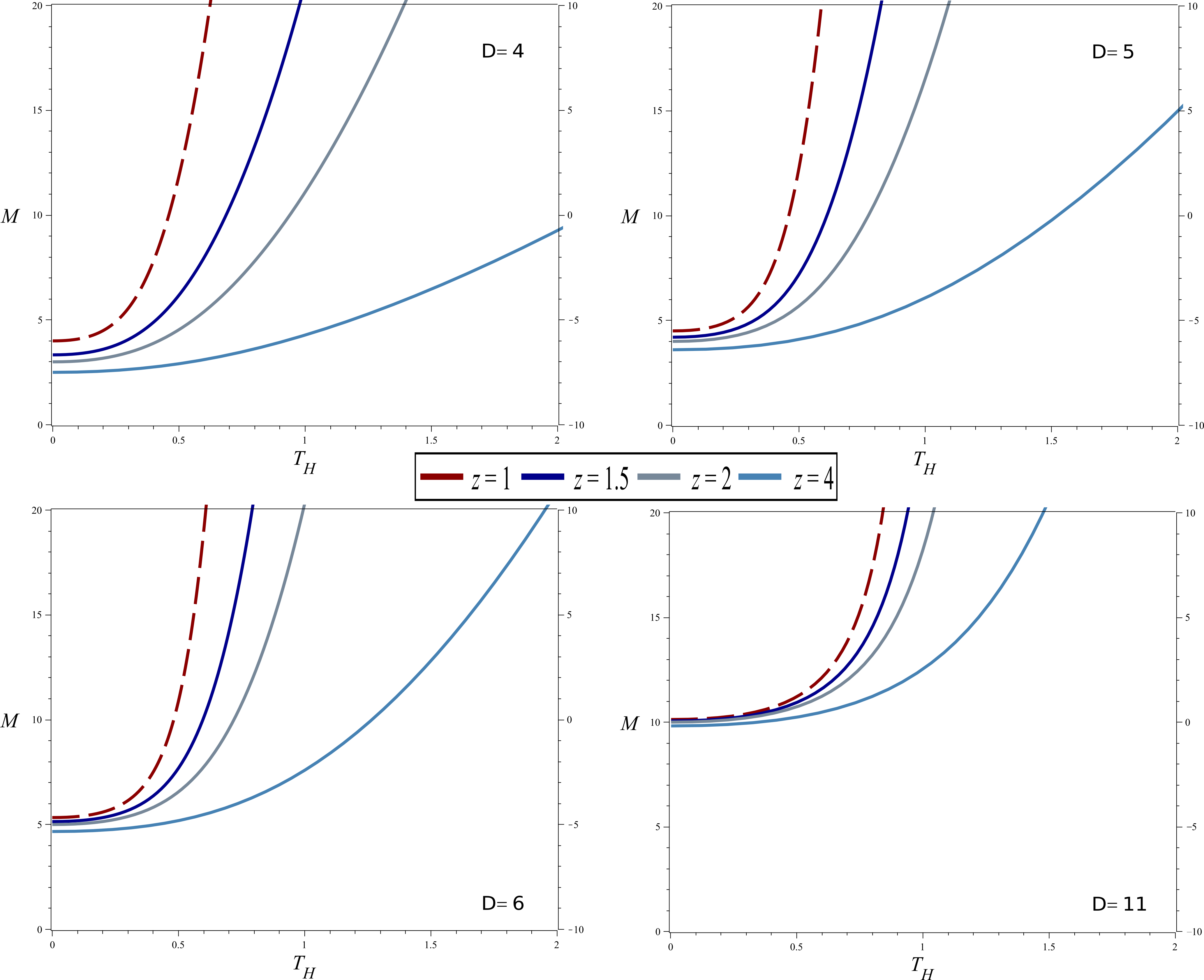
First, in Fig. 2 we display the curves of energy versus temperature for different values of $\displaystyle z$ and different dimensions. The most remarkable information provided by this plot is the fact that the energy for a given temperature value — with the rest of the variables fixed — is always higher for the isotropic (scalar-free) black hole with respect to any other scalarized ($\displaystyle z>1$) configuration.

$\displaystyle\displaystyle\mathcal{M}(T;z=1)>\mathcal{M}(T;z>1).$

(5.1)

An extension of the plot Fig. 2 to the region of negative temperatures displays a crossing point below which, the behavior is the inverse. Of course, we discard this region in compliance with the third law.

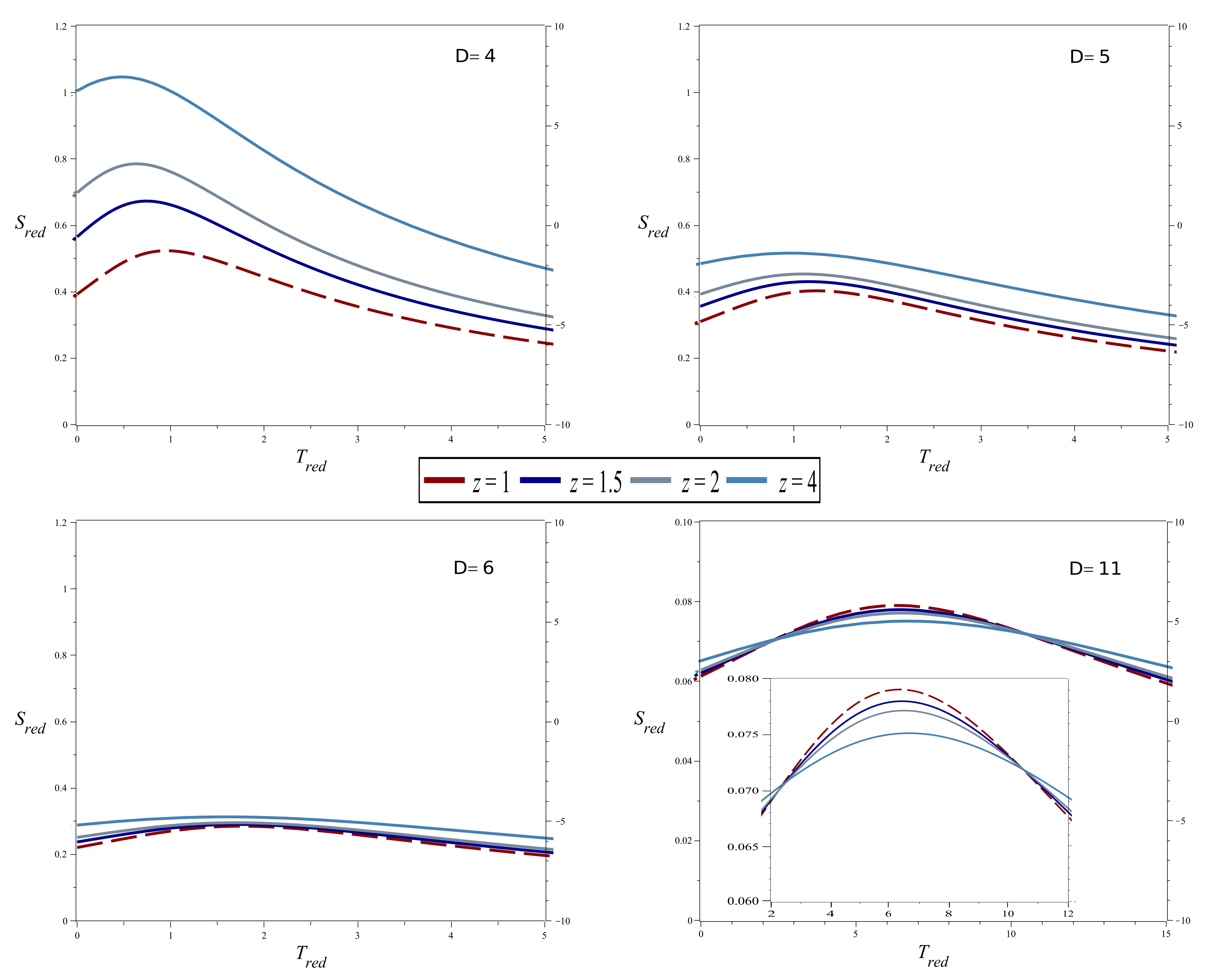
Looking for supplementary evidence, we portray the curves of reduced entropy versus reduced temperature in Fig. 3, similarly as done in [22, 44]. These quantities are defined as

$\displaystyle\displaystyle T_{\text{red}}:=\mathcal{M}T_{H},\qquad\quad S_{\text{red}}:=\frac{S}{\mathcal{M}^{2}}.$

(5.2)

Probing different dimensions, we realized that for $\displaystyle D=4,5,6$ the reduced entropy at given value of the reduced temperature is always higher in the scalarized (anisotropic) configuration compared to the scalar-free. This result is in agreement with the qualitative behavior of the energy curves, indicating that the anisotropic configuration are preferred,

$\displaystyle\displaystyle\mathcal{S_{\text{red}}}(T_{\text{red}};z=1)<\mathcal{S_{\text{red}}}(T_{\text{red}};z>1).$

(5.3)

However, the plot in $\displaystyle D=11$ shows an exchange region where the behavior is interchanged but it is recovered soon after. The crossing places of all different curves correspond to a single point which suggest a physical transition that urges for a deeper analysis.

The lower dimensional solution $\displaystyle D=3$ is left aside of the scalarization discussion. There is a main drawback in that case originated by the possible degeneracy of the scalar-free solution as discussed in Sec.3.2. Actually, it is reflected in the smoothness condition (3.11), which breaks down in said dimension and for $\displaystyle z=1$. Therefore, the comparison of the thermodynamical quantities for isotropic and anisotrpic configurations might be not well posed.

As a solution to a generalized Einstein-Maxwell-Dilaton theory, we have constructed a new family of exact Lifshitz black hole configurations. In such configurations, the existence of a nontrivial scalar field is a direct consequence of breaking the isotropic scaling symmetry between space and time ($\displaystyle z>1$). The scalar field trivializes at $\displaystyle z=1$ and becomes imaginary for $\displaystyle z<1$. The scalar-vector nonminimal coupling is mediated by the function (3.5), which is the most general for the given setup: a one-function static metric ansatz, and a purely electric vector potential. The obtained coupling can be understood as a nonlinear deviation from the standard dilaton coupling measured by the order of the new parameter $\displaystyle b$. In contrast to the limiting solution [33], the generalized dilaton coupling upholds a second horizon in our black hole, allowing then extremal configurations. It turns out that this solution passes the minimal tests to exhibit (spontaneous) scalarization at the cost of fixing the value of $\displaystyle b$ according to the smoothness condition (3.11). If it is imposed, the dilaton limit is lost and the effective couplings of the action obtain an unavoidable dependence on the critical exponent.

We have shown how the anisotropic black hole with a nontrivial scalar is energetically favored and, for a certain parameter region, it is also entropically favored as compared to the gravitating configuration with no scalar field. The region where the configurations are physically meaningful follows from the imposition of positive temperature, which exclude undesired thermodynamical behavior such as ill-defined physical quantities. Both cases, the one with a nontrivial scalar and the scalar-free black holes are continuously connected through the limit $\displaystyle z\rightarrow 1$. The other way around, the sudden emergence of a scalar field and a preferred thermodynamics are driven by a deviation from the isotropic scaling symmetry measured by $\displaystyle z>1$. More precisely, the amplitude of the scalar field and the entropy grow with a larger critical exponent. This phenomenon is remarkably similar to that of spontaneous scalarization where the evolution of the parameter into a threshold region triggers the transition of the configuration to a scalarized one. However the analogy is not exact. To speak of spontaneous scalarization, the smoothness condition should be fulfilled, and therefore $\displaystyle z$ will be effectively introduced in the action. As a result, varying the critical exponent means also changing the theory, and the scalarization process would not take place in the same moduli space.

Likewise, by regarding the dynamical exponent $\displaystyle z$ as a continuous parameter that can be varied towards the critical relativistic value $\displaystyle z=1$ — in which the scalar field vanishes — one can span several nonrelativistic quantum field theories with different physical properties. Since the scalarization phenomenon involves the emergence of a second order phase transition for the perturbations of the scalar field, it is interesting to explore its implications within the framework of the gravity/condensed matter theory correspondence. Work is currently in progress to elucidate the field theory physical meaning of this remarkable effect.

Despite the subtlety impeding the identification of the presented result as an analytical example of spontaneous black hole scalarization, our result suggests that breaking the isotropic scaling can be also a source for this effect such as rotation [20] or the violation of conformal invariance [28]. Of course, there are many directions to be explored as possible candidates capable of making compatible such scenarios. The most immediate one would be generalizing the scalar field dynamics, with the easiest case of including a self-interaction potential. This additional freedom could in principle remove the $\displaystyle z$ dependence from the action and allow the coexistence of both the scalarized and the scalar-free solution for a fixed coupling function.

Some words are in order relating to the stability of the quite general family of scalarizing asymptotically Lifshitz black hole configurations here constructed. In this regard, in [59] the authors studied real scalar field fluctuations about a $\displaystyle D$-dimensional family of black holes with Lifshitz asymptotics and generic critical exponent $\displaystyle z$. They showed that the latter are stable under scalar field perturbations for suitable boundary conditions. The study was performed by assuming a stationary separable ansatz for a probe scalar field in the background of an asymptotically Lifshitz black hole. The strategy was to compute the quasinormal mode frequencies and to impose incoming modes boundary conditions at the horizon and Dirichlet boundary conditions — equivalent to a vanishing scalar field — at infinity. It turns out that the imaginary part of these frequency modes always becomes negative, yielding a damping-off scalar field perturbation, provided a suitable Breitenlohner-Freedman bound is satisfied. Thus the stability of Lifshitz black holes is secured under this kind of perturbations. A similar result was accomplished in [60] for $\displaystyle D$-dimensional dilaton Lifshitz black holes coupled to Born-Infeld electrodynamics. Moreover, in [61] the authors numerically probed the stability of a $\displaystyle D=z=3$ Lifshitz black hole under both scalar and spinorial perturbations making use of quasinormal mode frequencies. Our asymptotically Lifshitz black hole field configuration possesses the required properties to ensure the kind of stability proved in [59] since our scalar field effective mass also obeys a Breitenlohner-Freedman bound. However, a complete stability analysis of asymptotically Lifshitz black hole spacetimes requires addressing the tensor perturbations as well, an interesting open question that deserves further attention. In this sense, we would like to mention that it seems feasible to carry out such an enterprise given that our gravitational action is simply the Einstein-Hilbert term. The task would become more arduous when considering higher-curvature terms, involving ghost fields, that have been considered previously in the literature.

All authors thank SNI for support. All authors are indebted to U. Nucamendi, E. Ayón-Beato, and M. Hassaïne for useful discussions. JAMZ thanks valuable comments from M. Lüben. AHA and DFHB acknowledge financial support by a CONACYT Grant No. A1-S-38041. DFHB is also grateful to CONACYT for a Postdoc por Mexico Grant No. 372516. JAMZ is supported by a grant of the Max Planck Society.

References

- [1] W. Israel, Phys. Rev. 164, 1776-1779 (1967); W. Israel and G. A. Wilson, J. Math. Phys. 13, 865-871 (1972).
- [2] D. C. Robinson, Phys. Rev. Lett. 34, 905-906 (1975); P. O. Mazur, J. Phys. A 15, 3173-3180 (1982); A. J. Amsel, G. T. Horowitz, D. Marolf and M. M. Roberts, Phys. Rev. D 81, 024033 (2010) [arXiv:0906.2367 [gr-qc]]; A. K. M. Masood-ul-Alam, [arXiv:1407.5381 [gr-qc]].
- [3] R. Ruffini and J. A. Wheeler, Phys. Today 24, no.1, 30 (1971) doi:10.1063/1.3022513
- [4] J. D. Bekenstein, Phys. Rev. D 5, 1239-1246 (1972); J. D. Bekenstein, Phys. Rev. D 5, 2403-2412 (1972); J. D. Bekenstein, Phys. Rev. Lett. 28, 452-455 (1972).
- [5] M. Heusler, Helv. Phys. Acta 69, no.4, 501-528 (1996) [arXiv:gr-qc/9610019 [gr-qc]]. J. D. Bekenstein, [arXiv:gr-qc/9605059 [gr-qc]]; E. Ayon-Beato, [arXiv:gr-qc/0210001 [gr-qc]].
- [6] A. Lahiri, Mod. Phys. Lett. A 8, 1549-1556 (1993) [arXiv:gr-qc/9207008 [gr-qc]]. J. D. Bekenstein, Phys. Rev. D 51, no.12, 6608 (1995) A. E. Mayo and J. D. Bekenstein, Phys. Rev. D 54, 5059-5069 (1996) [arXiv:gr-qc/9602057 [gr-qc]]. S. Bhattacharya and A. Lahiri, Phys. Rev. Lett. 99, 201101 (2007) [arXiv:gr-qc/0702006 [gr-qc]]. S. Bhattacharya and A. Lahiri, Phys. Rev. D 83, 124017 (2011) [arXiv:1102.0053 [gr-qc]].
- [7] K. A. Bronnikov, Acta Phys. Polon. B 4, 251-266 (1973) J. D. Bekenstein, Annals Phys. 82, 535-547 (1974) J. D. Bekenstein, Annals Phys. 91, 75-82 (1975)
- [8] P. Bizon, Phys. Rev. Lett. 64, 2844-2847 (1990); H. P. Kuenzle and A. K. M. Masood- ul- Alam, J. Math. Phys. 31, 928-935 (1990).
- [9] M. S. Volkov and D. V. Gal’tsov, Phys. Rept. 319, 1-83 (1999) [arXiv:hep-th/9810070 [hep-th]].
- [10] K. A. Bronnikov and Y. N. Kireev, Phys. Lett. A 67, 95-96 (1978)
- [11] P. Bizon and R. M. Wald, Phys. Lett. B 267, 173-174 (1991); Z. h. Zhou and N. Straumann, Nucl. Phys. B 360, 180-196 (1991).
- [12] A. Corichi, U. Nucamendi, and D. Sudarsky, Phys. Rev. D 62, 044046 (2000) [arXiv:gr-qc/0002078 [gr-qc]]; ibid. Phys. Rev. D 64, 107501 (2001) [arXiv:gr-qc/0106084 [gr-qc]].
- [13] A. Anabalon, Springer Proc. Phys. 157, 3-10 (2014) [arXiv:1211.2765 [gr-qc]]. C. A. R. Herdeiro and E. Radu, Int. J. Mod. Phys. D 24, no.09, 1542014 (2015) [arXiv:1504.08209 [gr-qc]].
- [14] Damour T, Esposito-Farèse G Class.Quant.Grav. 9 2176 (1992); T. Damour and G. Esposito-Farese, Phys. Rev. Lett. 70, 2220-2223 (1993) T. Damour and G. Esposito-Farese, Phys. Rev. D 54, 1474-1491 (1996) [arXiv:gr-qc/9602056 [gr-qc]].
- [15] T. Harada, Prog. Theor. Phys. 98, 359-379 (1997) doi:10.1143/PTP.98.359 [T. Harada, Phys. Rev. D 57, 4802-4811 (1998) doi:10.1103/PhysRevD.57.4802 [arXiv:gr-qc/9801049 [gr-qc]]; J. Novak, Phys. Rev. D 57, 4789-4801 (1998) [arXiv:gr-qc/9707041 [gr-qc]].
- [16] M. Salgado, D. Sudarsky and U. Nucamendi, Phys. Rev. D 58, 124003 (1998) [arXiv:gr-qc/9806070 [gr-qc]].
- [17] E. Berti, E. Barausse, V. Cardoso, L. Gualtieri, P. Pani, U. Sperhake, L. C. Stein, N. Wex, K. Yagi and T. Baker, et al. Class. Quant. Grav. 32, 243001 (2015) [arXiv:1501.07274 [gr-qc]]; E. Barausse, E. Berti, T. Hertog, S. A. Hughes, P. Jetzer, P. Pani, T. P. Sotiriou, N. Tamanini, H. Witek and K. Yagi, et al. Gen. Rel. Grav. 52, no.8, 81 (2020) doi:10.1007/s10714-020-02691-1 [arXiv:2001.09793 [gr-qc]].
- [18] P. V. P. Cunha, C. A. R. Herdeiro, E. Radu and H. F. Runarsson, Phys. Rev. Lett. 115, no.21, 211102 (2015) [arXiv:1509.00021 [gr-qc]]; M. Khodadi, A. Allahyari, S. Vagnozzi and D. F. Mota, JCAP 09, 026 (2020) [arXiv:2005.05992 [gr-qc]].
- [19] D. D. Doneva and S. S. Yazadjiev, Phys. Rev. Lett. 120, no.13, 131103 (2018) [arXiv:1711.01187 [gr-qc]]; H. O. Silva, J. Sakstein, L. Gualtieri, T. P. Sotiriou and E. Berti, Phys. Rev. Lett. 120, no.13, 131104 (2018) [arXiv:1711.02080 [gr-qc]]; G. Antoniou, A. Bakopoulos and P. Kanti, Phys. Rev. Lett. 120, no.13, 131102 (2018) [arXiv:1711.03390 [hep-th]].
- [20] A. Dima, E. Barausse, N. Franchini and T. P. Sotiriou, Phys. Rev. Lett. 125, no.23, 231101 (2020) [arXiv:2006.03095 [gr-qc]]; C. A. R. Herdeiro, E. Radu, H. O. Silva, T. P. Sotiriou and N. Yunes, [arXiv:2009.03904 [gr-qc]].
- [21] C. A. R. Herdeiro, E. Radu, N. Sanchis-Gual and J. A. Font, Phys. Rev. Lett. 121, no.10, 101102 (2018) [arXiv:1806.05190 [gr-qc]];
- [22] P. G. S. Fernandes, C. A. R. Herdeiro, A. M. Pombo, E. Radu and N. Sanchis-Gual, Class. Quant. Grav. 36, no.13, 134002 (2019) [erratum: Class. Quant. Grav. 37, no.4, 049501 (2020)] [arXiv:1902.05079 [gr-qc]].
- [23] Y. Brihaye and B. Hartmann, Phys. Lett. B 792, 244-250 (2019) [arXiv:1902.05760 [gr-qc]].
- [24] A. W. Whinnett and D.F. Torres, Astrophys. J. Lett. ApJ 603, L133 (2004) [arXiv:astro-ph/0401521 [astro-ph]].
- [25] M. Salgado, D. Sudarsky, and U. Nucamendi, Phys. Rev. D 70, 084027 (2004) [arXiv:gr-qc/0402126 [gr-qc]].
- [26] T. P. Sotiriou and V. Faraoni, Phys. Rev. Lett. 108, 081103 (2012) [arXiv:1109.6324 [gr-qc]]; V. Cardoso, I. P. Carucci, P. Pani and T. P. Sotiriou, Phys. Rev. Lett. 111, 111101 (2013) [arXiv:1308.6587 [gr-qc]]; V. Cardoso, I. P. Carucci, P. Pani and T. P. Sotiriou, Phys. Rev. D 88, 044056 (2013) [arXiv:1305.6936 [gr-qc]]; B. Kleihaus, J. Kunz and S. Yazadjiev, Phys. Lett. B 744, 406-412 (2015) [arXiv:1503.01672 [gr-qc]].
- [27] C. A. R. Herdeiro and E. Radu, Int. J. Mod. Phys. D 24, no.09, 1542014 (2015) [arXiv:1504.08209 [gr-qc]].
- [28] C. A. R. Herdeiro and E. Radu, Phys. Rev. D 99, no.8, 084039 (2019) [arXiv:1901.02953 [gr-qc]].
- [29] G. ’t Hooft and M. J. G. Veltman, Ann. Inst. H. Poincare Phys. Theor. A 20, 69-94 (1974); S. Weinberg, World Scientific (1993) 586 pp.
- [30] P. Horava, Phys. Rev. D 79, 084008 (2009) [arXiv:0901.3775 [hep-th]]; D. Blas, O. Pujolas and S. Sibiryakov, Phys. Rev. Lett. 104, 181302 (2010) [arXiv:0909.3525 [hep-th]]; H. Lu, J. Mei and C. N. Pope, Phys. Rev. Lett. 103, 091301 (2009) [arXiv:0904.1595 [hep-th]]; T. P. Sotiriou, J. Phys. Conf. Ser. 283, 012034 (2011) [arXiv:1010.3218 [hep-th]].
- [31] S. Kachru, X. Liu and M. Mulligan, Phys. Rev. D 78, 106005 (2008) [arXiv:0808.1725 [hep-th]].
- [32] S. Chadha and H. B. Nielsen, Nucl. Phys. B 217, 125-144 (1983)
- [33] M. Taylor, [arXiv:0812.0530 [hep-th]].
- [34] E. Ayon-Beato, A. Garbarz, G. Giribet and M. Hassaine, Phys. Rev. D 80, 104029 (2009) [arXiv:0909.1347 [hep-th]].
- [35] E. Ayon-Beato, A. Garbarz, G. Giribet and M. Hassaine, JHEP 04, 030 (2010) [arXiv:1001.2361 [hep-th]].
- [36] G. W. Gibbons and K. Maeda, Nucl. Phys. B 298, 741-775 (1988)
- [37] D. Garfinkle, G. T. Horowitz and A. Strominger, Phys. Rev. D 43, 3140 (1991) [erratum: Phys. Rev. D 45, 3888 (1992)]
- [38] A. Chamblin, R. Emparan, C. V. Johnson and R. C. Myers, Phys. Rev. D 60, 064018 (1999) [arXiv:hep-th/9902170 [hep-th]].
- [39] G. T. Horowitz (Ed.), “Black holes in higher dimensions,” Cambridge University Press (2012) 436.
- [40] A. Qadir and A. A. Siddiqui, Int. J. Mod. Phys. D 15, 1419-1440 (2006); R. Beig and A. A. Siddiqui, Class. Quant. Grav. 24, 5435-5439 (2007) [arXiv:1009.0586 [gr-qc]].
- [41] J. M. Maldacena, Int. J. Theor. Phys. 38, 1113-1133 (1999) [arXiv:hep-th/9711200 [hep-th]]; E. Witten, Adv. Theor. Math. Phys. 2, 253-291 (1998) [arXiv:hep-th/9802150 [hep-th]].
- [42] E. J. Brynjolfsson, U. H. Danielsson, L. Thorlacius and T. Zingg, J. Phys. A 43, 065401 (2010) [arXiv:0908.2611 [hep-th]]. R. G. Cai and H. Q. Zhang, Phys. Rev. D 81, 066003 (2010) [arXiv:0911.4867 [hep-th]]; Jun-Wang Lu, Ya-Bo Wu, Bao-Ping Dong, Yu Zhang, Phys. Let. B, 800 135079 (2020).
- [43] S. A. Hartnoll, A. Lucas, and S. Sachdev, [arXiv:1612.07324 [hep-th]].
- [44] D. Astefanesei, C. Herdeiro, J. Oliveira and E. Radu, JHEP 09, 186 (2020) [arXiv:2007.04153 [gr-qc]].
- [45] M. Banados, C. Teitelboim and J. Zanelli, Phys. Rev. Lett. 69, 1849-1851 (1992) [arXiv:hep-th/9204099 [hep-th]].
- [46] C. Martinez, C. Teitelboim and J. Zanelli, Phys. Rev. D 61, 104013 (2000) [arXiv:hep-th/9912259 [hep-th]].
- [47] S. Carlip, Class. Quant. Grav. 12, 2853-2880 (1995) [arXiv:gr-qc/9506079 [gr-qc]].
- [48] A. Garcia, [arXiv:hep-th/9909111 [hep-th]].
- [49] C. Keeler, JHEP 01, 067 (2014) [arXiv:1212.1728 [hep-th]].
- [50] P. Breitenlohner and D. Z. Freedman, Phys. Lett. B 115, 197-201 (1982); P. Breitenlohner and D. Z. Freedman, Annals Phys. 144, 249 (1982).
- [51] H. S. Liu and H. Lü, JHEP 12, 071 (2014) [arXiv:1410.6181 [hep-th]].
- [52] Y. Gim, W. Kim and S. H. Yi, JHEP 07, 002 (2014) [arXiv:1403.4704 [hep-th]].
- [53] W. Kim, S. Kulkarni and S. H. Yi, Phys. Rev. Lett. 111, no.8, 081101 (2013) [erratum: Phys. Rev. Lett. 112, no.7, 079902 (2014)] [arXiv:1306.2138 [hep-th]].
- [54] E. Ayón-Beato, M. Bravo-Gaete, F. Correa, M. Hassaïne, M. M. Juárez-Aubry and J. Oliva, Phys. Rev. D 91, no.6, 064006 (2015) [arXiv:1501.01244 [gr-qc]], E. Ayón-Beato, M. Bravo-Gaete, F. Correa, M. Hassaine and M. M. Juárez-Aubry, Phys. Rev. D 100, no.4, 044024 (2019) [arXiv:1904.09391 [hep-th]].
- [55] M. Bravo-Gaete, L. Guajardo and M. Hassaine, JHEP 04, 092 (2017) [arXiv:1702.02416 [hep-th]].
- [56] E. Ayón-Beato, M. Bravo-Gaete, F. Correa, M. Hassaine and M. M. Juárez-Aubry, Phys. Rev. D 100, no.4, 044024 (2019) [arXiv:1904.09391 [hep-th]].
- [57] M. Bravo-Gaete and M. M. Juárez-Aubry, Class. Quant. Grav. 37, no.7, 075016 (2020) [arXiv:2002.10520 [hep-th]].
- [58] S. Hyun, J. Jeong, S. A. Park and S. H. Yi, JHEP 10, 105 (2015) [arXiv:1507.03574 [hep-th]].
- [59] A. Giacomini, G. Giribet, M. Leston, J. Oliva and S. Ray, ’Phys. Rev. D 85, 124001 (2012) [arXiv:1203.0582 [hep-th]].
- [60] S. S. Hashemi, M. Kord Zangeneh and M. Faizal, Eur. Phys. J. C 80, no.2, 111 (2020) [arXiv:1901.11367 [hep-th]].
- [61] B. Cuadros-Melgar, J. de Oliveira and C. E. Pellicer, Phys. Rev. D 85, 024014 (2012) [arXiv:1110.4856 [hep-th]].
- [62] M. Bravo-Gaete and M. Hassaine, Phys. Rev. D 97, no.2, 024020 (2018) [arXiv:1710.02720 [hep-th]].