A Space-Time DPG Method for the Heat EquationThanks: This research was supported by the DFG through the CRC 1283 “Taming uncertainty and profiting from randomness and low regularity in analysis, stochastics and their applications”

Lars Diening and Johannes Storn L. Diening and J. StornDepartment of Mathematics, University of Bielefeld, Postfach 10 01 31, 33501 Bielefeld, Germany Email address: lars.diening@uni-bielefeld.de Email address: jstorn@math.uni-bielefeld.de

Abstract.

This paper introduces an ultra-weak space-time DPG method for the heat equation. We prove well-posedness of the variational formulation with broken test functions and verify quasi-optimality of a practical DPG scheme. Numerical experiments visualize beneficial properties of an adaptive and parabolically scaled mesh-refinement driven by the built-in error control of the DPG method.

Key words and phrases:

Parabolic PDEs, space-time FEM, DPG method, adaptivity

2020 Mathematics Subject Classification

35K20, 65M12, 65M15, 65M50, 65M60,

1. Introduction

This paper introduces an ultra-weak space-time discontinuous Petrov–Galerkin (DPG) method for the heat equation. More precisely, we reformulate the heat equation as a variational problem with discontinuous test functions. We prove the well-posedness of the variational problem and investigate a corresponding practical DPG scheme. The underlying mesh consists of time-space cylinders and allows for local adaptive mesh refinements in space-time. Our investigation shows quasi-optimality of the numerical approximation and leads to a reliable and efficient error estimator. We motivate the use of parabolically scaled mesh refinements (for which our mesh is well suited) and conclude our investigation with numerical experiments. These experiments indicate that our adaptive scheme is, in particular for non-smooth initial data, superior to state-of-the-art space-time methods.

Compared to classical time-marching schemes, simultaneous space-time finite element methods lead in general to significantly larger systems of equations. On the other hand, such schemes allow for massively parallel computations and quasi-optimal a priori estimates (a necessary requirement for optimally convergent adaptive schemes). Moreover, they are well-suited for adaptive mesh refinements simultaneously in space and time. These advantages have led to a growing interest in space-time methods for parabolic problems, see for example [Ste15, LMN16, Moo18]. A challenging difficulty is that known well-posed simultaneous space-time variational formulations of parabolic equations are not coercive. Hence, the resulting Petrov–Galerkin schemes require pairs of discrete trial and test spaces that satisfy the so-called Ladyzhenskaya–Babuška–Brezzi condition. Since the design of such pairs is nontrivial, Andreev suggests a minimal residual Petrov–Galerkin discretization [And13], see also [SW21]. An alternative approach are least-squares finite element methods (LSFEMs), suggested in [FK21] and [GS21]. LSFEMs are closely related to DPG schemes [Sto20]. However, the DPG method has some beneficial properties: it allows for a very flexible design of variational problems (see for example [FHS20]), might reduce to the discretization of traces (which simplifies the design of finite elements, see for example [FHN19]), and leads to instant stable adaptive schemes resulting in good rates of convergence even in pre-asymptotic regimes [BDS18, DS19, PD17]. These advantages motivate the investigation of space-time DPG methods. While space-time DPG methods for hyperbolic problems [EW19, GS19] and the Schrödinger equation [DGNS17] are already established, the existing literature on DPG methods for parabolic problems is, besides the numerical study in [EDCM14], limited to time-stepping schemes [FHSG17, RH20, FHK21]. Hence, this paper provides the first analytical foundation of space-time DPG methods for parabolic problems. To simplify the presentation as much as possible, we focus on the heat equation, even so most arguments extend to more general parabolic PDEs with ideas from [GS21].

This paper is organized as follows. Section 2 reformulates the heat equation as a first-order system and analyzes the resulting system with techniques from [GS21]. Section 3 designs an ultra-weak DPG method that bases on the first-order system from Section 2. The resulting variational problem is analyzed in Section 4. Section 5 briefly recalls abstract results from [CDG14, CDG16, GQ14] for the (practical) DPG method. These abstract results rely on the existence of a Fortin operator. Section 6.2 introduces a discretization and designs a suitable Fortin operator. The operator norm of the Fortin operator (and thus the DPG scheme) is stable for equally scaled meshes (the length of each cell in the mesh in time direction is equivalent to the diameter of the cell in space direction) and parabolically scaled meshes (the length of each cell in time direction is equivalent to the squared diameter of the cell in space direction). Section 6.5 and the numerical experiments in Section 7 show that the latter scaling is mandatory for singular solutions. In addition, the numerical experiments in Section 7 investigate an adaptive algorithm, driven by the built-in error control of the DPG method.

2. Heat Equation

Given a time-space cylinder $Q=\mathcal{I}\times\Omega$ with time-interval $\mathcal{I}=(0,T_{\textup{end}})\subset\mathbb{R}$ and bounded Lipschitz domain $\Omega\subset\mathbb{R}^{d}$ with boundary $\partial\Omega$ as well as a right-hand side $f\in L^{2}(Q)$ and some initial data $u_{0}\in L^{2}(\Omega)$ , the heat equation seeks the solution $u:Q\to\mathbb{R}$ to

(1)

\displaystyle\partial_{t}u-\Delta_{x}u=f\text{ in }Q,\qquad u(0,\mathbin{\mathchoice{\hbox to5.74991pt{\hfil\raise 0.0pt\hbox{\scalebox{.6}{\lower 0.0pt\hbox{$\displaystyle\bullet$}}}\hfil}}{\hbox to5.74991pt{\hfil\raise 0.0pt\hbox{\scalebox{.6}{\lower 0.0pt\hbox{$\textstyle\bullet$}}}\hfil}}{\hbox to5.28671pt{\hfil\raise 0.0pt\hbox{\scalebox{.6}{\lower 0.0pt\hbox{$\scriptstyle\bullet$}}}\hfil}}{\hbox to5.1909pt{\hfil\raise 0.0pt\hbox{\scalebox{.6}{\lower 0.0pt\hbox{$\scriptscriptstyle\bullet$}}}\hfil}}})=u_{0}\text{ in }\Omega,\qquad u=0\text{ on }\mathcal{I}\times\partial\Omega.

Let $\nabla_{x}=(\partial_{x_{1}},\dots,\partial_{x_{d}})$ denote the gradient with respect to the space directions $x_{1},\dots,x_{d}$ and set the divergence operator $\textup{div}\,(v,\tau)\coloneqq\partial_{t}v+\textup{div}_{x}\,\tau=\partial_{t}v+\partial_{x_{1}}\tau_{1}+\dots+\partial_{x_{d}}\tau_{d}$ for scalar valued functions $v$ and vector valued functions $\tau=(\tau_{1},\dots,\tau_{d})$ . The new unknown $\sigma\coloneqq-\nabla_{x}u$ leads in (1) to the first-order system

(2)

\displaystyle\begin{aligned} \textup{div}\,(u,\sigma)&=f&&\text{in }Q,&\qquad\nabla_{x}u+\sigma&=0&&\text{in }Q,\\ \qquad u(0,\mathbin{\mathchoice{\hbox to5.74991pt{\hfil\raise 0.0pt\hbox{\scalebox{.6}{\lower 0.0pt\hbox{$\displaystyle\bullet$}}}\hfil}}{\hbox to5.74991pt{\hfil\raise 0.0pt\hbox{\scalebox{.6}{\lower 0.0pt\hbox{$\textstyle\bullet$}}}\hfil}}{\hbox to5.28671pt{\hfil\raise 0.0pt\hbox{\scalebox{.6}{\lower 0.0pt\hbox{$\scriptstyle\bullet$}}}\hfil}}{\hbox to5.1909pt{\hfil\raise 0.0pt\hbox{\scalebox{.6}{\lower 0.0pt\hbox{$\scriptscriptstyle\bullet$}}}\hfil}}})&=u_{0}&&\text{in }\Omega,&\qquad u&=0&&\text{on }\mathcal{I}\times\partial\Omega.\end{aligned}

The differential operators in (2) are understood in a weak sense and lead to the space

\displaystyle U\coloneqq\big\{(v,\tau)\in L^{2}(Q)\times L^{2}(Q;\mathbb{R}^{d})\mid\nabla_{x}v\in L^{2}(Q;\mathbb{R}^{d})\text{ and }\textup{div}\,(v,\tau)\in L^{2}(Q)\big\}.

The space $U$ is a Hilbert space with norm, for all $(v,\tau)\in U$ ,

\displaystyle\lVert(v,\tau)\rVert_{U}^{2}\coloneqq\lVert\nabla_{x}v\rVert_{L^{2}(Q)}^{2}+\lVert(v,\tau)\rVert_{L^{2}(Q)}^{2}+\lVert\textup{div}\,(v,\tau)\rVert_{L^{2}(Q)}^{2},

where $\lVert\mathbin{\mathchoice{\hbox to5.74991pt{\hfil\raise 0.0pt\hbox{\scalebox{.6}{\lower 0.0pt\hbox{$\displaystyle\bullet$}}}\hfil}}{\hbox to5.74991pt{\hfil\raise 0.0pt\hbox{\scalebox{.6}{\lower 0.0pt\hbox{$\textstyle\bullet$}}}\hfil}}{\hbox to5.28671pt{\hfil\raise 0.0pt\hbox{\scalebox{.6}{\lower 0.0pt\hbox{$\scriptstyle\bullet$}}}\hfil}}{\hbox to5.1909pt{\hfil\raise 0.0pt\hbox{\scalebox{.6}{\lower 0.0pt\hbox{$\scriptscriptstyle\bullet$}}}\hfil}}}\rVert_{L^{2}(Q)}^{2}\coloneqq\langle\mathbin{\mathchoice{\hbox to5.74991pt{\hfil\raise 0.0pt\hbox{\scalebox{.6}{\lower 0.0pt\hbox{$\displaystyle\bullet$}}}\hfil}}{\hbox to5.74991pt{\hfil\raise 0.0pt\hbox{\scalebox{.6}{\lower 0.0pt\hbox{$\textstyle\bullet$}}}\hfil}}{\hbox to5.28671pt{\hfil\raise 0.0pt\hbox{\scalebox{.6}{\lower 0.0pt\hbox{$\scriptstyle\bullet$}}}\hfil}}{\hbox to5.1909pt{\hfil\raise 0.0pt\hbox{\scalebox{.6}{\lower 0.0pt\hbox{$\scriptscriptstyle\bullet$}}}\hfil}}},\mathbin{\mathchoice{\hbox to5.74991pt{\hfil\raise 0.0pt\hbox{\scalebox{.6}{\lower 0.0pt\hbox{$\displaystyle\bullet$}}}\hfil}}{\hbox to5.74991pt{\hfil\raise 0.0pt\hbox{\scalebox{.6}{\lower 0.0pt\hbox{$\textstyle\bullet$}}}\hfil}}{\hbox to5.28671pt{\hfil\raise 0.0pt\hbox{\scalebox{.6}{\lower 0.0pt\hbox{$\scriptstyle\bullet$}}}\hfil}}{\hbox to5.1909pt{\hfil\raise 0.0pt\hbox{\scalebox{.6}{\lower 0.0pt\hbox{$\scriptscriptstyle\bullet$}}}\hfil}}}\rangle_{L^{2}(Q)}\coloneqq\int_{Q}\mathbin{\mathchoice{\hbox to5.74991pt{\hfil\raise 0.0pt\hbox{\scalebox{.6}{\lower 0.0pt\hbox{$\displaystyle\bullet$}}}\hfil}}{\hbox to5.74991pt{\hfil\raise 0.0pt\hbox{\scalebox{.6}{\lower 0.0pt\hbox{$\textstyle\bullet$}}}\hfil}}{\hbox to5.28671pt{\hfil\raise 0.0pt\hbox{\scalebox{.6}{\lower 0.0pt\hbox{$\scriptstyle\bullet$}}}\hfil}}{\hbox to5.1909pt{\hfil\raise 0.0pt\hbox{\scalebox{.6}{\lower 0.0pt\hbox{$\scriptscriptstyle\bullet$}}}\hfil}}}\cdot\mathbin{\mathchoice{\hbox to5.74991pt{\hfil\raise 0.0pt\hbox{\scalebox{.6}{\lower 0.0pt\hbox{$\displaystyle\bullet$}}}\hfil}}{\hbox to5.74991pt{\hfil\raise 0.0pt\hbox{\scalebox{.6}{\lower 0.0pt\hbox{$\textstyle\bullet$}}}\hfil}}{\hbox to5.28671pt{\hfil\raise 0.0pt\hbox{\scalebox{.6}{\lower 0.0pt\hbox{$\scriptstyle\bullet$}}}\hfil}}{\hbox to5.1909pt{\hfil\raise 0.0pt\hbox{\scalebox{.6}{\lower 0.0pt\hbox{$\scriptscriptstyle\bullet$}}}\hfil}}}\,\mathrm{d}x$ denotes the squared $L^{2}$ norm. We include the boundary condition $u=0$ on $\mathcal{I}\times\partial\Omega$ by testing with non-compactly supported functions. This leads to the subspace $U_{0}\subset U$ . More precisely, let $C^{\infty}(\overline{Q};\mathbb{R}^{d})$ denote the space of infinitely often differentiable vector-valued functions on the closure $\overline{Q}$ of $Q$ , then a function ${\mathbf{v}}=(v,\tau)$ is in $U_{0}$ if and only if $(v,\tau)\in U$ and

(3)

\displaystyle\langle\nabla_{x}v,\chi\rangle_{L^{2}(Q)}

\displaystyle=-\langle v,\textup{div}_{x}\,\chi\rangle_{L^{2}(Q)}\qquad\text{for all }\chi\in C^{\infty}(\overline{Q};\mathbb{R}^{d}).

Simple arguments (hence we skip the proof) yield the following alternative characterization of $U$ and $U_{0}$ .

Lemma 1 (Relation to Bochner spaces).

The Sobolev spaces $U$ and $U_{0}$ equal the Bochner spaces from [GS21], that is

	$\displaystyle U$	$\displaystyle=\{(v,\tau)\in L^{2}(\mathcal{I};H^{1}(\Omega))\times L^{2}(Q;\mathbb{R}^{d})\mid\textup{div}\,(v,\tau)\in L^{2}(Q)\},$
	$\displaystyle U_{0}$	$\displaystyle=\{(v,\tau)\in L^{2}(\mathcal{I};H_{0}^{1}(\Omega))\times L^{2}(Q;\mathbb{R}^{d})\mid\textup{div}\,(v,\tau)\in L^{2}(Q)\}.$

The following lemma from [ABV13, Lem. 2] and [GS21, Lem. 2.1] bounds the dual norm $\lVert\mathbin{\mathchoice{\hbox to5.74991pt{\hfil\raise 0.0pt\hbox{\scalebox{.6}{\lower 0.0pt\hbox{$\displaystyle\bullet$}}}\hfil}}{\hbox to5.74991pt{\hfil\raise 0.0pt\hbox{\scalebox{.6}{\lower 0.0pt\hbox{$\textstyle\bullet$}}}\hfil}}{\hbox to5.28671pt{\hfil\raise 0.0pt\hbox{\scalebox{.6}{\lower 0.0pt\hbox{$\scriptstyle\bullet$}}}\hfil}}{\hbox to5.1909pt{\hfil\raise 0.0pt\hbox{\scalebox{.6}{\lower 0.0pt\hbox{$\scriptscriptstyle\bullet$}}}\hfil}}}\rVert_{L^{2}(\mathcal{I};H^{-1}(\Omega))}$ of $\lVert\mathbin{\mathchoice{\hbox to5.74991pt{\hfil\raise 0.0pt\hbox{\scalebox{.6}{\lower 0.0pt\hbox{$\displaystyle\bullet$}}}\hfil}}{\hbox to5.74991pt{\hfil\raise 0.0pt\hbox{\scalebox{.6}{\lower 0.0pt\hbox{$\textstyle\bullet$}}}\hfil}}{\hbox to5.28671pt{\hfil\raise 0.0pt\hbox{\scalebox{.6}{\lower 0.0pt\hbox{$\scriptstyle\bullet$}}}\hfil}}{\hbox to5.1909pt{\hfil\raise 0.0pt\hbox{\scalebox{.6}{\lower 0.0pt\hbox{$\scriptscriptstyle\bullet$}}}\hfil}}}\rVert_{L^{2}(\mathcal{I};H^{1}_{0}(\Omega))}=\lVert\nabla_{x}\,\mathbin{\mathchoice{\hbox to5.74991pt{\hfil\raise 0.0pt\hbox{\scalebox{.6}{\lower 0.0pt\hbox{$\displaystyle\bullet$}}}\hfil}}{\hbox to5.74991pt{\hfil\raise 0.0pt\hbox{\scalebox{.6}{\lower 0.0pt\hbox{$\textstyle\bullet$}}}\hfil}}{\hbox to5.28671pt{\hfil\raise 0.0pt\hbox{\scalebox{.6}{\lower 0.0pt\hbox{$\scriptstyle\bullet$}}}\hfil}}{\hbox to5.1909pt{\hfil\raise 0.0pt\hbox{\scalebox{.6}{\lower 0.0pt\hbox{$\scriptscriptstyle\bullet$}}}\hfil}}}\rVert_{L^{2}(Q)}$ for the time derivative $\partial_{t}v$ and so leads to a further characterization of the space $U_{0}$ . The lemma involves the Friedrichs constant $C_{\Omega}<\infty$ with

(4)

\displaystyle\lVert\xi\rVert^{2}_{L^{2}(\Omega)}\leq C_{\Omega}\lVert\nabla_{x}\xi\rVert^{2}_{L^{2}(\Omega)}\qquad\text{for all }\xi\in H^{1}_{0}(\Omega).

Lemma 2 (Control of time derivative).

All ${\mathbf{v}}\coloneqq(v,\tau)\in U_{0}$ satisfy

\displaystyle\lVert\partial_{t}v\rVert^{2}_{L^{2}(\mathcal{I};H^{-1}(\Omega))}\leq 2\,\max\{1,C_{\Omega}\}\,\lVert{\mathbf{v}}\rVert^{2}_{U}.

Proof.

Let ${\mathbf{v}}=(v,\tau)\in U_{0}$ . Its divergence reads $\textup{div}\,{\mathbf{v}}=\textup{div}\,(v,\tau)=\partial_{t}v+\textup{div}_{x}\,\tau$ . This identity and the triangle inequality yield

		$\displaystyle\lVert\partial_{t}v\rVert^{2}_{L^{2}(\mathcal{I};H^{-1}(\Omega))}\leq 2\,\lVert\textup{div}\,(v,\tau)\rVert_{L^{2}(\mathcal{I};H^{-1}(\Omega))}^{2}+2\,\lVert\textup{div}_{x}\,\tau\rVert_{L^{2}(\mathcal{I};H^{-1}(\Omega))}^{2}$
		$\displaystyle\quad\leq 2C_{\Omega}\lVert\textup{div}\,(v,\tau)\rVert_{L^{2}(Q)}^{2}+2\,\lVert\tau\rVert_{L^{2}(Q)}^{2}\leq 2\,\max\{1,C_{\Omega}\}\,\lVert{\mathbf{v}}\rVert^{2}_{U}.\qed$

As a consequence of Lemma 2, we have $v\in L^{2}(\mathcal{I};H^{1}_{0}(\Omega))\cap H^{1}(\mathcal{I};H^{-1}(\Omega))$ for all $(v,\tau)\in U_{0}$ . Hence, the space $U_{0}$ equals the ansatz space in [FK21]

\displaystyle U_{0}=\{(v,\tau)\in\big(L^{2}(\mathcal{I};H_{0}^{1}(\Omega))\cap H^{1}(\mathcal{I};H^{-1}(\Omega))\big)\times L^{2}(Q;\mathbb{R}^{d})\mid\textup{div}\,(v,\tau)\in L^{2}(Q)\}.

Moreover, the continuous embedding

\displaystyle L^{2}(\mathcal{I};H^{1}_{0}(\Omega))\cap H^{1}(\mathcal{I};H^{-1}(\Omega))\hookrightarrow C(\overline{\mathcal{I}};L^{2}(\Omega))

(see for example [DL92, p. 473, Thm. 1]) proves the existence of well-defined traces $\gamma_{0}{\mathbf{v}}\coloneqq\gamma_{0}v\coloneqq v(0,\mathbin{\mathchoice{\hbox to5.74991pt{\hfil\raise 0.0pt\hbox{\scalebox{.6}{\lower 0.0pt\hbox{$\displaystyle\bullet$}}}\hfil}}{\hbox to5.74991pt{\hfil\raise 0.0pt\hbox{\scalebox{.6}{\lower 0.0pt\hbox{$\textstyle\bullet$}}}\hfil}}{\hbox to5.28671pt{\hfil\raise 0.0pt\hbox{\scalebox{.6}{\lower 0.0pt\hbox{$\scriptstyle\bullet$}}}\hfil}}{\hbox to5.1909pt{\hfil\raise 0.0pt\hbox{\scalebox{.6}{\lower 0.0pt\hbox{$\scriptscriptstyle\bullet$}}}\hfil}}})$ and $\gamma_{T_{\textup{end}}}{\mathbf{v}}\coloneqq\gamma_{T_{\textup{end}}}v\coloneqq v(T_{\textup{end}},\mathbin{\mathchoice{\hbox to5.74991pt{\hfil\raise 0.0pt\hbox{\scalebox{.6}{\lower 0.0pt\hbox{$\displaystyle\bullet$}}}\hfil}}{\hbox to5.74991pt{\hfil\raise 0.0pt\hbox{\scalebox{.6}{\lower 0.0pt\hbox{$\textstyle\bullet$}}}\hfil}}{\hbox to5.28671pt{\hfil\raise 0.0pt\hbox{\scalebox{.6}{\lower 0.0pt\hbox{$\scriptstyle\bullet$}}}\hfil}}{\hbox to5.1909pt{\hfil\raise 0.0pt\hbox{\scalebox{.6}{\lower 0.0pt\hbox{$\scriptscriptstyle\bullet$}}}\hfil}}})$ in $L^{2}(\Omega)$ for all ${\mathbf{v}}=(v,\tau)\in U_{0}$ . Define for all $(v,\tau)\in U$ the operators

(5)

\displaystyle\begin{aligned} A(v,\tau)&\coloneqq\begin{pmatrix}\partial_{t}&\textup{div}_{x}\\ \nabla_{x}&\textup{id}\end{pmatrix}\begin{pmatrix}v\\ \tau\end{pmatrix}=\begin{pmatrix}\textup{div}\,(v,\tau)\\ \nabla_{x}v+\tau\end{pmatrix},\\ A^{*}(v,\tau)&\coloneqq\begin{pmatrix}-\partial_{t}&-\textup{div}_{x}\\ -\nabla_{x}&\textup{id}\end{pmatrix}\begin{pmatrix}v\\ \tau\end{pmatrix}=\begin{pmatrix}-\textup{div}\,(v,\tau)\\ -\nabla_{x}v+\tau\end{pmatrix}.\end{aligned}

Note that the space $U$ equals the space $H(A,Q)\coloneqq\{{\mathbf{v}}\in L^{2}(Q)\times L^{2}(Q;\mathbb{R}^{d})\mid A{\mathbf{v}}\in L^{2}(Q)\times L^{2}(Q;\mathbb{R}^{d})\}$ and the norm $\lVert\mathbin{\mathchoice{\hbox to5.74991pt{\hfil\raise 0.0pt\hbox{\scalebox{.6}{\lower 0.0pt\hbox{$\displaystyle\bullet$}}}\hfil}}{\hbox to5.74991pt{\hfil\raise 0.0pt\hbox{\scalebox{.6}{\lower 0.0pt\hbox{$\textstyle\bullet$}}}\hfil}}{\hbox to5.28671pt{\hfil\raise 0.0pt\hbox{\scalebox{.6}{\lower 0.0pt\hbox{$\scriptstyle\bullet$}}}\hfil}}{\hbox to5.1909pt{\hfil\raise 0.0pt\hbox{\scalebox{.6}{\lower 0.0pt\hbox{$\scriptscriptstyle\bullet$}}}\hfil}}}\rVert_{U}$ is equivalent to the graph norm $\lVert\mathbin{\mathchoice{\hbox to5.74991pt{\hfil\raise 0.0pt\hbox{\scalebox{.6}{\lower 0.0pt\hbox{$\displaystyle\bullet$}}}\hfil}}{\hbox to5.74991pt{\hfil\raise 0.0pt\hbox{\scalebox{.6}{\lower 0.0pt\hbox{$\textstyle\bullet$}}}\hfil}}{\hbox to5.28671pt{\hfil\raise 0.0pt\hbox{\scalebox{.6}{\lower 0.0pt\hbox{$\scriptstyle\bullet$}}}\hfil}}{\hbox to5.1909pt{\hfil\raise 0.0pt\hbox{\scalebox{.6}{\lower 0.0pt\hbox{$\scriptscriptstyle\bullet$}}}\hfil}}}\rVert_{H(A,Q)}\coloneqq(\lVert\mathbin{\mathchoice{\hbox to5.74991pt{\hfil\raise 0.0pt\hbox{\scalebox{.6}{\lower 0.0pt\hbox{$\displaystyle\bullet$}}}\hfil}}{\hbox to5.74991pt{\hfil\raise 0.0pt\hbox{\scalebox{.6}{\lower 0.0pt\hbox{$\textstyle\bullet$}}}\hfil}}{\hbox to5.28671pt{\hfil\raise 0.0pt\hbox{\scalebox{.6}{\lower 0.0pt\hbox{$\scriptstyle\bullet$}}}\hfil}}{\hbox to5.1909pt{\hfil\raise 0.0pt\hbox{\scalebox{.6}{\lower 0.0pt\hbox{$\scriptscriptstyle\bullet$}}}\hfil}}}\rVert_{L^{2}(Q)}^{2}+\lVert A\,\mathbin{\mathchoice{\hbox to5.74991pt{\hfil\raise 0.0pt\hbox{\scalebox{.6}{\lower 0.0pt\hbox{$\displaystyle\bullet$}}}\hfil}}{\hbox to5.74991pt{\hfil\raise 0.0pt\hbox{\scalebox{.6}{\lower 0.0pt\hbox{$\textstyle\bullet$}}}\hfil}}{\hbox to5.28671pt{\hfil\raise 0.0pt\hbox{\scalebox{.6}{\lower 0.0pt\hbox{$\scriptstyle\bullet$}}}\hfil}}{\hbox to5.1909pt{\hfil\raise 0.0pt\hbox{\scalebox{.6}{\lower 0.0pt\hbox{$\scriptscriptstyle\bullet$}}}\hfil}}}\rVert_{L^{2}(Q)}^{2})^{1/2}$ . Moreover, we have the following.

Theorem 3 (Equivalence of norms).

For all ${\mathbf{v}}=(v,\tau)\in U_{0}$ we have

(6)

\displaystyle\begin{aligned} \lVert A{\mathbf{v}}\rVert_{L^{2}(Q)}^{2}+\lVert\gamma_{0}{\mathbf{v}}\rVert_{L^{2}(\Omega)}^{2}\eqsim\lVert{\mathbf{v}}\rVert_{U}^{2}\eqsim\lVert A^{*}{\mathbf{v}}\rVert_{L^{2}(Q)}^{2}+\lVert\gamma_{T_{\textup{end}}}{\mathbf{v}}\rVert_{L^{2}(\Omega)}^{2}.\end{aligned}

In particular, there exists a constant $c_{\mathbf{L}}>0$ with

(7)

\displaystyle c_{\mathbf{L}}\lVert{\mathbf{v}}\rVert^{2}_{L^{2}(Q)}\leq\lVert A{\mathbf{v}}\rVert_{L^{2}(Q)}^{2}+\lVert\gamma_{0}{\mathbf{v}}\rVert_{L^{2}(\Omega)}^{2}\qquad\text{for all }{\mathbf{v}}\in U_{0}.

Proof.

The equivalence $\lVert A{\mathbf{v}}\rVert_{L^{2}(Q)}^{2}+\lVert\gamma_{0}{\mathbf{v}}\rVert_{L^{2}(\Omega)}^{2}\eqsim\lVert{\mathbf{v}}\rVert_{U}^{2}$ for all ${\mathbf{v}}\in U_{0}$ is a special case of [GS21, Thm. 2.3]. The proof exploits the equivalence of norms

(8)

\displaystyle\lVert\partial_{t}v-\Delta_{x}v\rVert_{L^{2}(\mathcal{I};H^{-1}(\Omega))}+\lVert\gamma_{0}v\rVert_{L^{2}(\Omega)}\eqsim\lVert\nabla_{x}v\rVert_{L^{2}(Q)}+\lVert\partial_{t}v\rVert_{L^{2}(\mathcal{I};H^{-1}(\Omega))}

for all $v\in L^{2}(\mathcal{I};H^{1}_{0}(\Omega))\times H^{1}(\mathcal{I};H^{-1}(\Omega))$ [SS09, Thm. 5.1]. Similar arguments lead to the equivalence $\lVert{\mathbf{v}}\rVert_{U}^{2}\eqsim\lVert A^{*}{\mathbf{v}}\rVert_{L^{2}(Q)}^{2}+\lVert\gamma_{T_{\textup{end}}}{\mathbf{v}}\rVert_{L^{2}(\Omega)}^{2}$ . ∎

Remark 4 (Dependence on $T_{\textup{end}}$ ).

Let $v\in L^{2}(\mathcal{I};H^{1}_{0}(\Omega))\cap H^{1}(\mathcal{I};H^{-1}(\Omega))$ , then we have for all $t\in\mathcal{I}$ the identity

\displaystyle\lVert v(0,\mathbin{\mathchoice{\hbox to5.74991pt{\hfil\raise 0.0pt\hbox{\scalebox{.6}{\lower 0.0pt\hbox{$\displaystyle\bullet$}}}\hfil}}{\hbox to5.74991pt{\hfil\raise 0.0pt\hbox{\scalebox{.6}{\lower 0.0pt\hbox{$\textstyle\bullet$}}}\hfil}}{\hbox to5.28671pt{\hfil\raise 0.0pt\hbox{\scalebox{.6}{\lower 0.0pt\hbox{$\scriptstyle\bullet$}}}\hfil}}{\hbox to5.1909pt{\hfil\raise 0.0pt\hbox{\scalebox{.6}{\lower 0.0pt\hbox{$\scriptscriptstyle\bullet$}}}\hfil}}})\rVert_{L^{2}(\Omega)}^{2}

\displaystyle=\lVert v(t,\mathbin{\mathchoice{\hbox to5.74991pt{\hfil\raise 0.0pt\hbox{\scalebox{.6}{\lower 0.0pt\hbox{$\displaystyle\bullet$}}}\hfil}}{\hbox to5.74991pt{\hfil\raise 0.0pt\hbox{\scalebox{.6}{\lower 0.0pt\hbox{$\textstyle\bullet$}}}\hfil}}{\hbox to5.28671pt{\hfil\raise 0.0pt\hbox{\scalebox{.6}{\lower 0.0pt\hbox{$\scriptstyle\bullet$}}}\hfil}}{\hbox to5.1909pt{\hfil\raise 0.0pt\hbox{\scalebox{.6}{\lower 0.0pt\hbox{$\scriptscriptstyle\bullet$}}}\hfil}}})\rVert_{L^{2}(\Omega)}^{2}+2\int_{0}^{t}\langle\partial_{t}v(s,\mathbin{\mathchoice{\hbox to5.74991pt{\hfil\raise 0.0pt\hbox{\scalebox{.6}{\lower 0.0pt\hbox{$\displaystyle\bullet$}}}\hfil}}{\hbox to5.74991pt{\hfil\raise 0.0pt\hbox{\scalebox{.6}{\lower 0.0pt\hbox{$\textstyle\bullet$}}}\hfil}}{\hbox to5.28671pt{\hfil\raise 0.0pt\hbox{\scalebox{.6}{\lower 0.0pt\hbox{$\scriptstyle\bullet$}}}\hfil}}{\hbox to5.1909pt{\hfil\raise 0.0pt\hbox{\scalebox{.6}{\lower 0.0pt\hbox{$\scriptscriptstyle\bullet$}}}\hfil}}}),v(s,\mathbin{\mathchoice{\hbox to5.74991pt{\hfil\raise 0.0pt\hbox{\scalebox{.6}{\lower 0.0pt\hbox{$\displaystyle\bullet$}}}\hfil}}{\hbox to5.74991pt{\hfil\raise 0.0pt\hbox{\scalebox{.6}{\lower 0.0pt\hbox{$\textstyle\bullet$}}}\hfil}}{\hbox to5.28671pt{\hfil\raise 0.0pt\hbox{\scalebox{.6}{\lower 0.0pt\hbox{$\scriptstyle\bullet$}}}\hfil}}{\hbox to5.1909pt{\hfil\raise 0.0pt\hbox{\scalebox{.6}{\lower 0.0pt\hbox{$\scriptscriptstyle\bullet$}}}\hfil}}})\rangle_{H^{-1}(\Omega),H^{1}_{0}(\Omega)}\,\mathrm{d}s.

Averaging the previous identity over the time interval $\mathcal{I}$ yields

\displaystyle\lVert v(0,\mathbin{\mathchoice{\hbox to5.74991pt{\hfil\raise 0.0pt\hbox{\scalebox{.6}{\lower 0.0pt\hbox{$\displaystyle\bullet$}}}\hfil}}{\hbox to5.74991pt{\hfil\raise 0.0pt\hbox{\scalebox{.6}{\lower 0.0pt\hbox{$\textstyle\bullet$}}}\hfil}}{\hbox to5.28671pt{\hfil\raise 0.0pt\hbox{\scalebox{.6}{\lower 0.0pt\hbox{$\scriptstyle\bullet$}}}\hfil}}{\hbox to5.1909pt{\hfil\raise 0.0pt\hbox{\scalebox{.6}{\lower 0.0pt\hbox{$\scriptscriptstyle\bullet$}}}\hfil}}})\rVert_{L^{2}(\Omega)}^{2}

\displaystyle\leq\left(1+\frac{C_{\Omega}}{T_{\textup{end}}}\right)\lVert\nabla_{x}v\rVert_{L^{2}(Q)}^{2}+\lVert\partial_{t}v\rVert_{L^{2}(\mathcal{I};H^{-1}(\Omega))}^{2}.

Using this estimate in the proof of (8) (and so of Theorem 3) leads to a constant $C_{1}\approx 1+1/T_{\textup{end}}$ (with equivalence constants depending on $\Omega$ but not $T_{\textup{end}}$ ) which satisfies for all ${\mathbf{v}}\in U_{0}$

	$\displaystyle\lVert A{\mathbf{v}}\rVert_{L^{2}(Q)}^{2}+\lVert\gamma_{0}{\mathbf{v}}\rVert_{L^{2}(\Omega)}^{2}$	$\displaystyle\leq C_{1}\lVert{\mathbf{v}}\rVert_{U}^{2},$
	$\displaystyle\lVert A^{*}{\mathbf{v}}\rVert_{L^{2}(Q)}^{2}+\lVert\gamma_{T_{\textup{end}}}{\mathbf{v}}\rVert_{L^{2}(\Omega)}^{2}$	$\displaystyle\leq C_{1}\lVert{\mathbf{v}}\rVert_{U}^{2}.$

The hidden constant in the “ $\ \gtrsim$ ” estimate in (8) is uniformly bounded for all $T_{\textup{end}}>0$ , which can be seen by a simple adjustment of the proof in [SS09, Thm. 5.1]. This observation yields the existence of $T_{\textup{end}}$ -independent constants $0<c_{\mathbf{L}}$ in (7) and $C_{2}<\infty$ with, for all ${\mathbf{v}}\in U_{0}$ ,

	$\displaystyle\lVert{\mathbf{v}}\rVert_{U}^{2}$	$\displaystyle\leq C_{2}(\lVert A{\mathbf{v}}\rVert_{L^{2}(Q)}^{2}+\lVert\gamma_{0}{\mathbf{v}}\rVert_{L^{2}(\Omega)}^{2})$
	$\displaystyle\lVert{\mathbf{v}}\rVert_{U}^{2}$	$\displaystyle\leq C_{2}(\lVert A^{*}{\mathbf{v}}\rVert_{L^{2}(Q)}^{2}+\lVert\gamma_{T_{\textup{end}}}{\mathbf{v}}\rVert_{L^{2}(\Omega)}^{2}).$

The equivalence of norms shows injectivity and continuity of the linear mapping

\displaystyle(A\,\mathbin{\mathchoice{\hbox to5.74991pt{\hfil\raise 0.0pt\hbox{\scalebox{.6}{\lower 0.0pt\hbox{$\displaystyle\bullet$}}}\hfil}}{\hbox to5.74991pt{\hfil\raise 0.0pt\hbox{\scalebox{.6}{\lower 0.0pt\hbox{$\textstyle\bullet$}}}\hfil}}{\hbox to5.28671pt{\hfil\raise 0.0pt\hbox{\scalebox{.6}{\lower 0.0pt\hbox{$\scriptstyle\bullet$}}}\hfil}}{\hbox to5.1909pt{\hfil\raise 0.0pt\hbox{\scalebox{.6}{\lower 0.0pt\hbox{$\scriptscriptstyle\bullet$}}}\hfil}}},\gamma_{0}\,\mathbin{\mathchoice{\hbox to5.74991pt{\hfil\raise 0.0pt\hbox{\scalebox{.6}{\lower 0.0pt\hbox{$\displaystyle\bullet$}}}\hfil}}{\hbox to5.74991pt{\hfil\raise 0.0pt\hbox{\scalebox{.6}{\lower 0.0pt\hbox{$\textstyle\bullet$}}}\hfil}}{\hbox to5.28671pt{\hfil\raise 0.0pt\hbox{\scalebox{.6}{\lower 0.0pt\hbox{$\scriptstyle\bullet$}}}\hfil}}{\hbox to5.1909pt{\hfil\raise 0.0pt\hbox{\scalebox{.6}{\lower 0.0pt\hbox{$\scriptscriptstyle\bullet$}}}\hfil}}}):U_{0}\to\big(L^{2}(Q)\times L^{2}(Q;\mathbb{R}^{d})\big)\times L^{2}(\Omega).

Surjectivity of this mapping is proven in [GS21, Thm. 2.3]. Combining these properties shows well-posedness of the following parabolic problem. Given ${\mathbf{f}}\in L^{2}(Q)\times L^{2}(Q;\mathbb{R}^{d})$ and $u_{0}\in L^{2}(\Omega)$ , seek ${\mathbf{u}}\in U_{0}$ with

(9)

\displaystyle\begin{aligned} A{\mathbf{u}}={\mathbf{f}}\qquad\text{and}\qquad\gamma_{0}{\mathbf{u}}=u_{0}.\end{aligned}

The problem in (2) corresponds to the right-hand side ${\mathbf{f}}=(f,0)^{\top}$ with $f\in L^{2}(Q)$ . It is possible to include right-hand sides $f\in L^{2}(\mathcal{I};H^{-1}(\Omega))$ by defining suitable right-hand sides ${\mathbf{f}}\in L^{2}(Q)\times L^{2}(Q;\mathbb{R}^{d})$ , see [GS21, Prop. 2.5] for details. We conclude this section with proving additional properties of the space $U_{0}$ .

Lemma 5 (Alternative characterizations of $U_{0}$ ).

A function ${\mathbf{v}}$ is in $U_{0}$ if and only if ${\mathbf{v}}\in L^{2}(Q)\times L^{2}(Q;\mathbb{R}^{d})$ and there exists a function $\Theta\in L^{2}(Q)\times L^{2}(Q;\mathbb{R}^{d})$ with

\displaystyle\langle\Theta,{\mathbf{w}}\rangle_{L^{2}(Q)}=\langle{\mathbf{v}},A^{*}{\mathbf{w}}\rangle_{L^{2}(Q)}\qquad\text{for all }{\mathbf{w}}\in C_{c}^{\infty}(Q)\times C^{\infty}(\overline{Q};\mathbb{R}^{d}).

Alternatively, a function ${\mathbf{v}}$ is in $U_{0}$ if and only if ${\mathbf{v}}\in L^{2}(Q)\times L^{2}(Q;\mathbb{R}^{d})$ and there exists a function $\Xi\in L^{2}(Q)\times L^{2}(Q;\mathbb{R}^{d})$ with

\displaystyle\langle\Xi,{\mathbf{w}}\rangle_{L^{2}(Q)}=\langle{\mathbf{v}},A{\mathbf{w}}\rangle_{L^{2}(Q)}\qquad\text{for all }{\mathbf{w}}\in C_{c}^{\infty}(Q)\times C^{\infty}(\overline{Q};\mathbb{R}^{d}).

The functions satisfy $\Theta=A{\mathbf{v}}$ and $\Xi=A^{*}{\mathbf{v}}$ .

Proof.

The definition of $A$ and $A^{*}$ as well as the characterization of the space $U_{0}$ by the weak divergence div and gradient $\nabla_{x}$ in (3) yield this lemma. ∎

The following result shows density of smooth functions in $U_{0}$ . The set of smooth functions involves the space $C_{D}^{\infty}(\overline{Q})\coloneqq\{v\in C^{\infty}(\overline{Q})\mid v|_{\mathcal{I}\times\partial\Omega}=0\}$ . A similar result is proven in [ABV13, Lem. 4] with mollification techniques. Our proof relies on the definition of weak derivatives.

Lemma 6 (Dense subspace).

Smooth functions are dense in $U_{0}$ , that is,

\displaystyle U_{0}=\overline{C_{D}^{\infty}(\overline{Q})\times C^{\infty}(\overline{Q};\mathbb{R}^{d})}^{\lVert\mathbin{\mathchoice{\hbox to4.82535pt{\hfil\raise 0.0pt\hbox{\scalebox{.6}{\lower 0.0pt\hbox{$\displaystyle\bullet$}}}\hfil}}{\hbox to4.82535pt{\hfil\raise 0.0pt\hbox{\scalebox{.6}{\lower 0.0pt\hbox{$\textstyle\bullet$}}}\hfil}}{\hbox to3.6594pt{\hfil\raise 0.0pt\hbox{\scalebox{.6}{\lower 0.0pt\hbox{$\scriptstyle\bullet$}}}\hfil}}{\hbox to3.21216pt{\hfil\raise 0.0pt\hbox{\scalebox{.6}{\lower 0.0pt\hbox{$\scriptscriptstyle\bullet$}}}\hfil}}}\rVert_{U}}.

Proof.

This proof verifies the following alternative characterization of dense subspaces: A subspace $\mathcal{U}_{0}$ of $U_{0}$ is dense if and only if every element $\zeta$ in the dual $U_{0}^{*}$ of $U_{0}$ that vanishes on $\mathcal{U}_{0}$ also vanishes on $U_{0}$ .

Let $\zeta\in U_{0}^{*}$ with $\zeta({\mathbf{w}})=0$ for all ${\mathbf{w}}\in C_{D}^{\infty}(\overline{Q})\times C^{\infty}(\overline{Q};\mathbb{R}^{d})$ . Theorem 3 and the Riesz representation theorem imply the existence of a function ${\mathbf{v}}\in U_{0}$ with $\zeta=\langle A{\mathbf{v}},A\,\mathbin{\mathchoice{\hbox to5.74991pt{\hfil\raise 0.0pt\hbox{\scalebox{.6}{\lower 0.0pt\hbox{$\displaystyle\bullet$}}}\hfil}}{\hbox to5.74991pt{\hfil\raise 0.0pt\hbox{\scalebox{.6}{\lower 0.0pt\hbox{$\textstyle\bullet$}}}\hfil}}{\hbox to5.28671pt{\hfil\raise 0.0pt\hbox{\scalebox{.6}{\lower 0.0pt\hbox{$\scriptstyle\bullet$}}}\hfil}}{\hbox to5.1909pt{\hfil\raise 0.0pt\hbox{\scalebox{.6}{\lower 0.0pt\hbox{$\scriptscriptstyle\bullet$}}}\hfil}}}\rangle_{L^{2}(Q)}+\langle\gamma_{0}{\mathbf{v}},\gamma_{0}\mathbin{\mathchoice{\hbox to5.74991pt{\hfil\raise 0.0pt\hbox{\scalebox{.6}{\lower 0.0pt\hbox{$\displaystyle\bullet$}}}\hfil}}{\hbox to5.74991pt{\hfil\raise 0.0pt\hbox{\scalebox{.6}{\lower 0.0pt\hbox{$\textstyle\bullet$}}}\hfil}}{\hbox to5.28671pt{\hfil\raise 0.0pt\hbox{\scalebox{.6}{\lower 0.0pt\hbox{$\scriptstyle\bullet$}}}\hfil}}{\hbox to5.1909pt{\hfil\raise 0.0pt\hbox{\scalebox{.6}{\lower 0.0pt\hbox{$\scriptscriptstyle\bullet$}}}\hfil}}}\rangle_{L^{2}(\Omega)}$ . We have

(10)

\displaystyle\langle A{\mathbf{v}},A{\mathbf{w}}\rangle_{L^{2}(Q)}+\langle\gamma_{0}{\mathbf{v}},\gamma_{0}{\mathbf{w}}\rangle_{L^{2}(\Omega)}=0\quad\text{for all }{\mathbf{w}}\in C^{\infty}_{D}(\overline{Q})\times C^{\infty}(\overline{Q};\mathbb{R}^{d}).

Testing with functions in the subspace $C^{\infty}_{c}(Q)\times C^{\infty}(\overline{Q};\mathbb{R}^{d})$ reveals

\displaystyle\langle A{\mathbf{v}},A{\mathbf{w}}\rangle_{L^{2}(Q)}=0\qquad\text{for all }{\mathbf{w}}\in C^{\infty}_{c}(Q)\times C^{\infty}(\overline{Q};\mathbb{R}^{d}).

The second characterization in Lemma 5 shows that $A^{*}A{\mathbf{v}}=0$ and $\Theta\coloneqq A{\mathbf{v}}\in U_{0}$ . Set the subspace $C^{\infty}_{D,0}(\overline{Q})\coloneqq\{w\in C^{\infty}_{D}(\overline{Q})\mid\gamma_{0}w=0\}$ . We have

\displaystyle\langle\Theta,A{\mathbf{w}}\rangle_{L^{2}(Q)}=\langle\Theta,A{\mathbf{w}}\rangle_{L^{2}(Q)}-\langle A^{*}\Theta,{\mathbf{w}}\rangle_{L^{2}(Q)}=0\quad\text{for all }{\mathbf{w}}\in C_{D,0}^{\infty}(\overline{Q})\times\{0\}.

This is equivalent to $\langle\textup{div}\,\Theta,w\rangle_{L^{2}(Q)}+\langle\Theta,\nabla w\rangle_{L^{2}(Q)}=0$ for all $w\in C_{D,0}^{\infty}(\overline{Q})$ . Thus, the normal trace of $\Theta\in U_{0}\subset H(\textup{div},Q)$ on $\{T_{\textup{end}}\}\times\Omega$ must be equal to zero, that is, the trace $\gamma_{T_{\textup{end}}}\Theta=0$ . The combination of $\gamma_{T_{\textup{end}}}\Theta=0$ , $A^{*}\Theta=0$ , and Theorem 3 implies $0=\Theta=A{\mathbf{v}}$ . This identity leads in (10) to

\displaystyle\langle\gamma_{0}{\mathbf{v}},w\rangle_{L^{2}(\Omega)}=0\qquad\text{for all }w\in C^{\infty}_{c}(\Omega).

Thus, the trace $\gamma_{0}{\mathbf{v}}=0$ . Combining this identity with $A{\mathbf{v}}=0$ and Theorem 3 shows ${\mathbf{v}}=0$ and concludes the proof. ∎

Define the spaces

(11)

\displaystyle C^{\infty}_{D,T_{\textup{end}}}(\overline{Q})\coloneqq\{w\in C^{\infty}_{D}(\overline{Q})\mid\gamma_{T_{\textup{end}}}w=0\}\ \text{ and }\ U_{00}\coloneqq\{{\mathbf{v}}\in U_{0}\mid\gamma_{0}{\mathbf{v}}=0\}.

Lemma 7 (Alternative characterization of $U_{00}$ ).

A function ${\mathbf{v}}$ is in $U_{00}$ if and only if ${\mathbf{v}}\in L^{2}(Q)\times L^{2}(Q;\mathbb{R}^{d})$ and there exists a function $\Theta\in L^{2}(Q)\times L^{2}(Q;\mathbb{R}^{d})$ with

(12)

\displaystyle\langle\Theta,{\mathbf{w}}\rangle_{L^{2}(Q)}=\langle{\mathbf{v}},A^{*}{\mathbf{w}}\rangle_{L^{2}(Q)}\qquad\text{for all }{\mathbf{w}}\in C_{D,T_{\textup{end}}}^{\infty}(\overline{Q})\times C^{\infty}(\overline{Q};\mathbb{R}^{d}).

The function $\Theta$ satisfies $\Theta=A{\mathbf{v}}$ .

Proof.

Let ${\mathbf{v}}=(v,\tau)\in L^{2}(Q)\times L^{2}(Q;\mathbb{R}^{d})$ with (12). Since $C_{c}^{\infty}(Q)\subset C_{D,T_{\textup{end}}}^{\infty}(\overline{Q})$ , Lemma 5 proves that ${\mathbf{v}}\in U_{0}$ . Moreover, (12) implies

(13)

\displaystyle\langle\textup{div}\,{\mathbf{v}},w\rangle_{L^{2}(Q)}=-\langle{\mathbf{v}},\nabla w\rangle_{L^{2}(Q)}\qquad\text{for all }w\in C_{D,T_{\textup{end}}}^{\infty}(\overline{Q}).

An integration by parts shows for sufficiently smooth functions ${\mathbf{v}}$ the equivalence of (13) and (with outer unit normal vector $\nu$ )

\displaystyle 0=\int_{\partial Q}{\mathbf{v}}\cdot\nu\,w\,\mathrm{d}s=-\int_{\Omega}\gamma_{0}v\,\gamma_{0}w\,\mathrm{d}s\qquad\text{for all }w\in C_{D,T_{\textup{end}}}^{\infty}(\overline{Q}).

In particular, the integral $\int_{\Omega}\gamma_{0}v\,w\,\mathrm{d}x=0$ for all $w\in C_{c}^{\infty}(\Omega)$ . This proves $\gamma_{0}v=0$ for all sufficiently smooth functions $v$ . Density arguments (which apply due to Lemma 6) conclude the proof. ∎

3. Design of the DPG Method

This section reformulates the problem in (9) as a variational problem with test functions that are discontinuous across the interfaces of some given partition $\mathcal{T}$ of the time-space cylinder $Q$ . The design follows [CDG16] with abstractly defined traces as in [EG06, DGNS17, Sto20]. Recall the definition of the (formally adjoint) operator

\displaystyle A^{*}\coloneqq\begin{pmatrix}-\partial_{t}&-\textup{div}_{x}\\ -\nabla_{x}&\textup{id}\end{pmatrix}.

For all $K\in\mathcal{T}$ define the domain of the operator $A^{*}$ as

		$\displaystyle H(A^{},K)\coloneqq\{{\mathbf{w}}\in L^{2}(K)\times L^{2}(K;\mathbb{R}^{d})\mid A^{}{\mathbf{w}}\in L^{2}(K)\}$
		$\displaystyle\quad\hphantom{:}=\{(w,\chi)\in L^{2}(K)\times L^{2}(K;\mathbb{R}^{d})\mid\textup{div}\,(w,\chi)\in L^{2}(K)\text{ and }\nabla_{x}w\in L^{2}(K;\mathbb{R}^{d})\}.$

Define the space of broken functions

	$\displaystyle H(A^{*},\mathcal{T})$	$\displaystyle\coloneqq\{{\mathbf{w}}\in L^{2}(Q)\times L^{2}(Q;\mathbb{R}^{d})\mid{\mathbf{w}}\|_{K}\in H(A^{*},K)\text{ for all }K\in\mathcal{T}\},$
	$\displaystyle Y$	$\displaystyle\coloneqq H(A^{*},\mathcal{T})\times L^{2}(\Omega).$

Let $A^{*}_{h}$ denote the element-wise application of $A^{*}$ , that is,

\displaystyle(A^{*}_{h}{\mathbf{w}})|_{K}\coloneqq A^{*}({\mathbf{w}}|_{K})\qquad\text{for all }{\mathbf{w}}\in H(A^{*},\mathcal{T})\text{ and }K\in\mathcal{T}.

For all functions $({\mathbf{w}},\xi),(\widetilde{{\mathbf{w}}},\tilde{\xi})$ in the Hilbert space $Y$ the inner product reads

(14)

\displaystyle\langle{\mathbf{w}},\xi;\widetilde{{\mathbf{w}}},\tilde{\xi}\rangle_{Y}\coloneqq\langle{\mathbf{w}},\widetilde{{\mathbf{w}}}\rangle_{L^{2}(Q)}+\langle A_{h}^{*}{\mathbf{w}},A_{h}^{*}\widetilde{{\mathbf{w}}}\rangle_{L^{2}(Q)}+\langle\xi,\tilde{\xi}\rangle_{L^{2}(\Omega)}.

The induced norm reads

\displaystyle\lVert({\mathbf{w}},\xi)\rVert_{Y}^{2}\coloneqq\lVert{\mathbf{w}}\rVert_{L^{2}(Q)}^{2}+\lVert A_{h}^{*}{\mathbf{w}}\rVert_{L^{2}(Q)}^{2}+\lVert\xi\rVert_{L^{2}(\Omega)}^{2}.

A multiplication of (9) by a broken test function and an integration over $Q$ and $\Omega$ lead to the variational problem: Seek ${\mathbf{u}}\in U_{0}$ such that for all $({\mathbf{w}},\xi)\in Y$

(15)

\displaystyle\langle A{\mathbf{u}},{\mathbf{w}}\rangle_{L^{2}(Q)}+\langle\gamma_{0}{\mathbf{u}},\xi\rangle_{L^{2}(\Omega)}=\langle{\mathbf{f}},{\mathbf{w}}\rangle_{L^{2}(Q)}+\langle u_{0},\xi\rangle_{L^{2}(\Omega)}.

Define for all ${\mathbf{v}}=(v,\tau)\in U_{0}$ and $({\mathbf{w}},\xi)\in Y$ with ${\mathbf{w}}=(w,\chi)$ the pairing

(16)

\displaystyle\begin{aligned} \langle\gamma_{A}{\mathbf{v}},({\mathbf{w}},\xi)\rangle_{\partial\mathcal{T}}&\coloneqq\langle A{\mathbf{v}},{\mathbf{w}}\rangle_{L^{2}(Q)}-\langle{\mathbf{v}},A^{*}_{h}{\mathbf{w}}\rangle_{L^{2}(Q)}+\langle\gamma_{0}{\mathbf{v}},\xi\rangle_{L^{2}(\Omega)}\\ &\hphantom{:}=\sum_{K\in\mathcal{T}}\big(\langle\textup{div}\,{\mathbf{v}},w\rangle_{L^{2}(K)}+\langle\nabla_{x}v,\chi\rangle_{L^{2}(K)}+\langle v,\textup{div}\,{\mathbf{w}}\rangle_{L^{2}(K)}\\ &\ \quad\qquad+\langle\tau,\nabla_{x}w\rangle_{L^{2}(K)}\big)+\langle\gamma_{0}v,\xi\rangle_{L^{2}(\Omega)}.\end{aligned}

This pairing defines the bounded (trace) operator $\gamma_{A}:U_{0}\to Y^{*}$ with

\displaystyle\gamma_{A}{\mathbf{v}}\coloneqq\langle\gamma_{A}{\mathbf{v}},\mathbin{\mathchoice{\hbox to5.74991pt{\hfil\raise 0.0pt\hbox{\scalebox{.6}{\lower 0.0pt\hbox{$\displaystyle\bullet$}}}\hfil}}{\hbox to5.74991pt{\hfil\raise 0.0pt\hbox{\scalebox{.6}{\lower 0.0pt\hbox{$\textstyle\bullet$}}}\hfil}}{\hbox to5.28671pt{\hfil\raise 0.0pt\hbox{\scalebox{.6}{\lower 0.0pt\hbox{$\scriptstyle\bullet$}}}\hfil}}{\hbox to5.1909pt{\hfil\raise 0.0pt\hbox{\scalebox{.6}{\lower 0.0pt\hbox{$\scriptscriptstyle\bullet$}}}\hfil}}}\rangle_{\partial\mathcal{T}}.

Set the functional $F({\mathbf{w}},\xi)\coloneqq\langle{\mathbf{f}},{\mathbf{w}}\rangle_{L^{2}(Q)}+\langle u_{0},\xi\rangle_{L^{2}(\Omega)}$ for all $({\mathbf{w}},\xi)\in Y$ . By design the variational problem in (15) is equivalent to

\displaystyle\langle{\mathbf{u}},A^{*}_{h}{\mathbf{w}}\rangle_{L^{2}(Q)}+\langle\gamma_{A}{\mathbf{u}},({\mathbf{w}},\xi)\rangle_{\partial\mathcal{T}}=F({\mathbf{w}},\xi)\qquad\text{for all }({\mathbf{w}},\xi)\in Y.

We define the (trace) space $\Gamma(\partial\mathcal{T})\coloneqq\gamma_{A}U_{0}\subset Y^{*}$ as a subspace of the dual space $Y^{*}$ and set the product space

(17)

\displaystyle X\coloneqq\big(L^{2}(Q)\times L^{2}(Q;\mathbb{R}^{d})\big)\times\Gamma(\partial\mathcal{T}).

The space $X$ is a Hilbert space with the canonical product norm $(\lVert{\mathbf{v}}\rVert_{L^{2}(Q)}^{2}+\lVert{\mathbf{t}}\rVert_{Y^{*}}^{2})^{1/2}$ for all $({\mathbf{v}},{\mathbf{t}})\in X$ . Set for all $({\mathbf{v}},{\mathbf{t}})\in X$ and $({\mathbf{w}},\xi)\in Y$ the bilinear form $b:X\times Y\to\mathbb{R}$ as

(18)

\displaystyle b({\mathbf{v}},{\mathbf{t}};{\mathbf{w}},\xi)\coloneqq\langle{\mathbf{v}},A^{*}_{h}{\mathbf{w}}\rangle_{L^{2}(Q)}+\langle{\mathbf{t}},({\mathbf{w}},\xi)\rangle_{\partial\mathcal{T}}.

We introduce the trace ${\mathbf{s}}\coloneqq\gamma_{A}{\mathbf{u}}$ as new unknown. Then the ultra-weak broken variational formulation of (9) reads as follows.

Definition 8 (Variational formulation).

Given $F\in Y^{*}$ , we seek $({\mathbf{u}},{\mathbf{s}})\in X$ with

(19)

\displaystyle b({\mathbf{u}},{\mathbf{s}};{\mathbf{w}},\xi)=F({\mathbf{w}},\xi)\qquad\text{for all }({\mathbf{w}},\xi)\in Y.

We conclude this section with the proof of the equivalence of the variational problem (19) and the PDE in (9). The proof bases upon the following two lemmas.

Lemma 9 (Unbroken functions).

We have

\displaystyle\langle{\mathbf{t}},({\mathbf{w}},0)\rangle_{\partial\mathcal{T}}=0\qquad\text{for all }{\mathbf{t}}\in\Gamma(\partial\mathcal{T})\text{ and }{\mathbf{w}}\in C_{c}^{\infty}(Q)\times C^{\infty}(\overline{Q};\mathbb{R}^{d}).

Proof.

Let ${\mathbf{t}}\in\Gamma(\partial\mathcal{T})$ and ${\mathbf{w}}\in C_{c}^{\infty}(Q)\times C^{\infty}(\overline{Q};\mathbb{R}^{d})$ . The definition $\Gamma(\partial\mathcal{T})\coloneqq\gamma_{A}U_{0}$ yields the existence of a function ${\mathbf{q}}\in U_{0}$ with $\gamma_{A}{\mathbf{q}}={\mathbf{t}}$ . Lemma 5 implies

	$\displaystyle\langle{\mathbf{t}},({\mathbf{w}},0)\rangle_{\Gamma(\partial\mathcal{T})}$	$\displaystyle=\langle A{\mathbf{q}},{\mathbf{w}}\rangle_{L^{2}(Q)}-\langle{\mathbf{q}},A^{*}_{h}{\mathbf{w}}\rangle_{L^{2}(Q)}$
		$\displaystyle=\langle A{\mathbf{q}},{\mathbf{w}}\rangle_{L^{2}(Q)}-\langle{\mathbf{q}},A^{*}{\mathbf{w}}\rangle_{L^{2}(Q)}=0.\qed$

Lemma 10 (Identical traces).

Two traces ${\mathbf{t}},{\mathbf{r}}\in\Gamma(\partial\mathcal{T})$ are identical, if

(20)

\displaystyle\langle{\mathbf{t}},({\mathbf{w}},0)\rangle_{\partial\mathcal{T}}=\langle{\mathbf{r}},({\mathbf{w}},0)\rangle_{\partial\mathcal{T}}\qquad\text{for all }{\mathbf{w}}\in H(A^{*},\mathcal{T}).

Proof.

Recall the definition of the spaces $U_{00}$ and $C_{D,T_{\textup{end}}}^{\infty}(\overline{Q})$ in (11). Let ${\mathbf{v}}\in U_{0}$ with $\gamma_{A}{\mathbf{v}}={\mathbf{t}}$ and

\displaystyle\langle{\mathbf{t}},({\mathbf{w}},0)\rangle_{\partial\mathcal{T}}=0\qquad\text{for all }{\mathbf{w}}\in H(A^{*},\mathcal{T}).

This yields for all ${\mathbf{w}}\in C_{D,T_{\textup{end}}}^{\infty}(\overline{Q})\times C^{\infty}(\overline{Q};\mathbb{R}^{d})\subset H(A^{*},\mathcal{T})$ that

\displaystyle 0=\langle{\mathbf{t}},({\mathbf{w}},0)\rangle_{\partial\mathcal{T}}=\langle\gamma_{A}{\mathbf{v}},({\mathbf{w}},0)\rangle_{\partial\mathcal{T}}=\langle A{\mathbf{v}},{\mathbf{w}}\rangle_{L^{2}(Q)}-\langle{\mathbf{v}},A^{*}{\mathbf{w}}\rangle_{L^{2}(Q)}.

Thus Lemma 7 shows ${\mathbf{v}}\in U_{00}$ , that is, $\gamma_{0}{\mathbf{v}}=0$ . This proves

	$\displaystyle\langle{\mathbf{t}},({\mathbf{w}},\xi)\rangle_{\partial\mathcal{T}}$	$\displaystyle=\langle{\mathbf{t}},(0,\xi)\rangle_{\partial\mathcal{T}}=\langle\gamma_{A}{\mathbf{v}},(0,\xi)\rangle_{\partial\mathcal{T}}$
		$\displaystyle=\langle\gamma_{0}{\mathbf{v}},\xi\rangle_{L^{2}(\Omega)}=0\qquad\qquad\text{for all }({\mathbf{w}},\xi)\in Y.$

Since ${\mathbf{t}}\in Y^{*}$ , this shows the identity ${\mathbf{t}}=0$ . ∎

With the previous observations we can prove the following equivalence.

Theorem 11 (Equivalent problems).

If ${\mathbf{u}}\in U_{0}$ solves (9), then the pair $({\mathbf{u}},\gamma_{A}{\mathbf{u}})\in X$ solves (19). Conversely, if the pair $({\mathbf{u}},{\mathbf{s}})\in X$ solves (19), then ${\mathbf{s}}=\gamma_{A}{\mathbf{u}}$ and ${\mathbf{u}}\in U_{0}$ solves (9).

Proof.

It follows by the design of the variational problem (19) that any solution ${\mathbf{u}}\in U_{0}$ to (9) leads to a solution $({\mathbf{u}},\gamma_{A}{\mathbf{u}})\in X$ to (19). Vice versa, let $({\mathbf{u}},{\mathbf{s}})\in X$ solve (19). Lemma 5 and Lemma 9 show that testing with smooth functions $({\mathbf{w}},0)\in\big(C_{c}^{\infty}(Q)\times C^{\infty}(\overline{Q};\mathbb{R}^{d})\big)\times\{0\}\subset Y$ results in ${\mathbf{u}}\in U_{0}$ with $A{\mathbf{u}}={\mathbf{f}}$ . The combination of the integration by parts formula in (16) and the variational problem (19) shows for all $({\mathbf{w}},\xi)\in Y$ that

(21)

\displaystyle\begin{aligned} &\langle A{\mathbf{u}},{\mathbf{w}}\rangle_{L^{2}(Q)}+\langle\gamma_{0}{\mathbf{u}},\xi\rangle_{L^{2}(\Omega)}-\langle\gamma_{A}{\mathbf{u}},({\mathbf{w}},\xi)\rangle_{\partial\mathcal{T}}+\langle{\mathbf{s}},({\mathbf{w}},\xi)\rangle_{\partial\mathcal{T}}\\ &\hskip 113.81102pt=b({\mathbf{u}},{\mathbf{s}};{\mathbf{w}},\xi)=\langle{\mathbf{f}},{\mathbf{w}}\rangle_{L^{2}(Q)}+\langle u_{0},\xi\rangle_{L^{2}(\Omega)}.\end{aligned}

Using the identity $A{\mathbf{u}}={\mathbf{f}}$ and testing with $({\mathbf{w}},0)\in Y$ allows for the application of Lemma 10. This lemma shows that $\gamma_{A}{\mathbf{u}}={\mathbf{s}}$ . Testing in (21) with functions $(0,\xi)\in Y$ shows $\gamma_{0}{\mathbf{u}}=u_{0}$ and concludes the proof. ∎

4. Analysis of the Variational Problem

Since the seminal paper [CDG16] and its generalization in [DGNS17], the well-posedness of broken variational formulations is well understood. Our investigation follows [Sto20], which allows us to conclude sharp inf-sup and continuity constants.

Recall the definition of the product space $X$ in (17) and the definition of the inner product $\langle\mathbin{\mathchoice{\hbox to5.74991pt{\hfil\raise 0.0pt\hbox{\scalebox{.6}{\lower 0.0pt\hbox{$\displaystyle\bullet$}}}\hfil}}{\hbox to5.74991pt{\hfil\raise 0.0pt\hbox{\scalebox{.6}{\lower 0.0pt\hbox{$\textstyle\bullet$}}}\hfil}}{\hbox to5.28671pt{\hfil\raise 0.0pt\hbox{\scalebox{.6}{\lower 0.0pt\hbox{$\scriptstyle\bullet$}}}\hfil}}{\hbox to5.1909pt{\hfil\raise 0.0pt\hbox{\scalebox{.6}{\lower 0.0pt\hbox{$\scriptscriptstyle\bullet$}}}\hfil}}},\mathbin{\mathchoice{\hbox to5.74991pt{\hfil\raise 0.0pt\hbox{\scalebox{.6}{\lower 0.0pt\hbox{$\displaystyle\bullet$}}}\hfil}}{\hbox to5.74991pt{\hfil\raise 0.0pt\hbox{\scalebox{.6}{\lower 0.0pt\hbox{$\textstyle\bullet$}}}\hfil}}{\hbox to5.28671pt{\hfil\raise 0.0pt\hbox{\scalebox{.6}{\lower 0.0pt\hbox{$\scriptstyle\bullet$}}}\hfil}}{\hbox to5.1909pt{\hfil\raise 0.0pt\hbox{\scalebox{.6}{\lower 0.0pt\hbox{$\scriptscriptstyle\bullet$}}}\hfil}}}\rangle_{Y}$ in the Hilbert space $Y$ in (14). The Riesz representation theorem yields the existence of the so-called trial-to-test operator $T:X\to Y$ with

\displaystyle\langle T({\mathbf{v}},{\mathbf{t}}),({\mathbf{w}},\xi)\rangle_{Y}=b({\mathbf{v}},{\mathbf{t}};{\mathbf{w}},\xi)\qquad\text{for all }({\mathbf{v}},{\mathbf{t}})\in X\text{ and }({\mathbf{w}},\xi)\in Y.

The trial-to-test operator decomposes into $T({\mathbf{v}},{\mathbf{t}})=\big(T_{1}({\mathbf{v}},{\mathbf{t}}),T_{2}({\mathbf{t}})\big)\in Y$ , where $T_{2}$ is independent of ${\mathbf{v}}$ due to the definition of the inner product $\langle\mathbin{\mathchoice{\hbox to5.74991pt{\hfil\raise 0.0pt\hbox{\scalebox{.6}{\lower 0.0pt\hbox{$\displaystyle\bullet$}}}\hfil}}{\hbox to5.74991pt{\hfil\raise 0.0pt\hbox{\scalebox{.6}{\lower 0.0pt\hbox{$\textstyle\bullet$}}}\hfil}}{\hbox to5.28671pt{\hfil\raise 0.0pt\hbox{\scalebox{.6}{\lower 0.0pt\hbox{$\scriptstyle\bullet$}}}\hfil}}{\hbox to5.1909pt{\hfil\raise 0.0pt\hbox{\scalebox{.6}{\lower 0.0pt\hbox{$\scriptscriptstyle\bullet$}}}\hfil}}},\mathbin{\mathchoice{\hbox to5.74991pt{\hfil\raise 0.0pt\hbox{\scalebox{.6}{\lower 0.0pt\hbox{$\displaystyle\bullet$}}}\hfil}}{\hbox to5.74991pt{\hfil\raise 0.0pt\hbox{\scalebox{.6}{\lower 0.0pt\hbox{$\textstyle\bullet$}}}\hfil}}{\hbox to5.28671pt{\hfil\raise 0.0pt\hbox{\scalebox{.6}{\lower 0.0pt\hbox{$\scriptstyle\bullet$}}}\hfil}}{\hbox to5.1909pt{\hfil\raise 0.0pt\hbox{\scalebox{.6}{\lower 0.0pt\hbox{$\scriptscriptstyle\bullet$}}}\hfil}}}\rangle_{Y}$ and the bilinear form $b$ .

Remark 12 (Trial-to-test operator).

Given some discrete subspace $X_{h}\subset X$ and a norm $\lVert\mathbin{\mathchoice{\hbox to5.74991pt{\hfil\raise 0.0pt\hbox{\scalebox{.6}{\lower 0.0pt\hbox{$\displaystyle\bullet$}}}\hfil}}{\hbox to5.74991pt{\hfil\raise 0.0pt\hbox{\scalebox{.6}{\lower 0.0pt\hbox{$\textstyle\bullet$}}}\hfil}}{\hbox to5.28671pt{\hfil\raise 0.0pt\hbox{\scalebox{.6}{\lower 0.0pt\hbox{$\scriptstyle\bullet$}}}\hfil}}{\hbox to5.1909pt{\hfil\raise 0.0pt\hbox{\scalebox{.6}{\lower 0.0pt\hbox{$\scriptscriptstyle\bullet$}}}\hfil}}}\rVert_{X}$ in $X$ , the trial-to-test operator allows to compute an “optimal” test space $TX_{h}\subset Y$ that leads to a discrete inf-sup constant

\displaystyle\beta\coloneqq\inf_{x\in X\setminus\{0\}}\sup_{y\in Y\setminus\{0\}}\frac{b(x,y)}{\lVert x\rVert_{X}\lVert y\rVert_{Y}}\leq\beta_{h}\coloneqq\inf_{x_{h}\in X_{h}\setminus\{0\}}\sup_{y_{h}\in TX_{h}\setminus\{0\}}\frac{b(x_{h},y_{h})}{\lVert x_{h}\rVert_{X}\lVert y_{h}\rVert_{Y}}.

Hence, the inf-sup stability of the continuous problem yields the inf-sup stability of the discretized problem. This was an initial motivation for the development of the DPG scheme, see for example [DG10, DG11].

Recall the graph norm $\lVert\mathbin{\mathchoice{\hbox to5.74991pt{\hfil\raise 0.0pt\hbox{\scalebox{.6}{\lower 0.0pt\hbox{$\displaystyle\bullet$}}}\hfil}}{\hbox to5.74991pt{\hfil\raise 0.0pt\hbox{\scalebox{.6}{\lower 0.0pt\hbox{$\textstyle\bullet$}}}\hfil}}{\hbox to5.28671pt{\hfil\raise 0.0pt\hbox{\scalebox{.6}{\lower 0.0pt\hbox{$\scriptstyle\bullet$}}}\hfil}}{\hbox to5.1909pt{\hfil\raise 0.0pt\hbox{\scalebox{.6}{\lower 0.0pt\hbox{$\scriptscriptstyle\bullet$}}}\hfil}}}\rVert_{H(A,Q)}=(\lVert\mathbin{\mathchoice{\hbox to5.74991pt{\hfil\raise 0.0pt\hbox{\scalebox{.6}{\lower 0.0pt\hbox{$\displaystyle\bullet$}}}\hfil}}{\hbox to5.74991pt{\hfil\raise 0.0pt\hbox{\scalebox{.6}{\lower 0.0pt\hbox{$\textstyle\bullet$}}}\hfil}}{\hbox to5.28671pt{\hfil\raise 0.0pt\hbox{\scalebox{.6}{\lower 0.0pt\hbox{$\scriptstyle\bullet$}}}\hfil}}{\hbox to5.1909pt{\hfil\raise 0.0pt\hbox{\scalebox{.6}{\lower 0.0pt\hbox{$\scriptscriptstyle\bullet$}}}\hfil}}}\rVert^{2}_{L^{2}(Q)}+\lVert A\,\mathbin{\mathchoice{\hbox to5.74991pt{\hfil\raise 0.0pt\hbox{\scalebox{.6}{\lower 0.0pt\hbox{$\displaystyle\bullet$}}}\hfil}}{\hbox to5.74991pt{\hfil\raise 0.0pt\hbox{\scalebox{.6}{\lower 0.0pt\hbox{$\textstyle\bullet$}}}\hfil}}{\hbox to5.28671pt{\hfil\raise 0.0pt\hbox{\scalebox{.6}{\lower 0.0pt\hbox{$\scriptstyle\bullet$}}}\hfil}}{\hbox to5.1909pt{\hfil\raise 0.0pt\hbox{\scalebox{.6}{\lower 0.0pt\hbox{$\scriptscriptstyle\bullet$}}}\hfil}}}\rVert^{2}_{L^{2}(Q)})^{1/2}$ and define for all $({\mathbf{v}},{\mathbf{t}})\in X$ the (mesh-dependent) operator $\mathcal{E}({\mathbf{v}},{\mathbf{t}})\in L^{2}(Q)\times L^{2}(Q;\mathbb{R}^{d})$ by

\displaystyle\mathcal{E}({\mathbf{v}},{\mathbf{t}})

\displaystyle\coloneqq{\mathbf{v}}-A^{*}_{h}T_{1}({\mathbf{v}},{\mathbf{t}}).

Theorem 13 (Extension operator).

For all $({\mathbf{v}},{\mathbf{t}})\in X$ we have

(a)

$\mathcal{E}({\mathbf{v}},{\mathbf{t}})\in U_{0}$ with $A\mathcal{E}({\mathbf{v}},{\mathbf{t}})=T_{1}({\mathbf{v}},{\mathbf{t}})$ ,
(b)

$\gamma_{A}\mathcal{E}({\mathbf{v}},{\mathbf{t}})={\mathbf{t}}$ ,
(c)

$\lVert b({\mathbf{v}},{\mathbf{t}};\mathbin{\mathchoice{\hbox to5.74991pt{\hfil\raise 0.0pt\hbox{\scalebox{.6}{\lower 0.0pt\hbox{$\displaystyle\bullet$}}}\hfil}}{\hbox to5.74991pt{\hfil\raise 0.0pt\hbox{\scalebox{.6}{\lower 0.0pt\hbox{$\textstyle\bullet$}}}\hfil}}{\hbox to5.28671pt{\hfil\raise 0.0pt\hbox{\scalebox{.6}{\lower 0.0pt\hbox{$\scriptstyle\bullet$}}}\hfil}}{\hbox to5.1909pt{\hfil\raise 0.0pt\hbox{\scalebox{.6}{\lower 0.0pt\hbox{$\scriptscriptstyle\bullet$}}}\hfil}}})\rVert^{2}_{Y^{*}}=\lVert{\mathbf{v}}-\mathcal{E}({\mathbf{v}},{\mathbf{t}})\rVert^{2}_{L^{2}(Q)}+\lVert A\mathcal{E}({\mathbf{v}},{\mathbf{t}})\rVert_{L^{2}(Q)}^{2}+\lVert\gamma_{0}\mathcal{E}({\mathbf{v}},{\mathbf{t}})\rVert_{L^{2}(\Omega)}^{2}$ ,
(d)

$\lVert\mathcal{E}(0,{\mathbf{t}})\rVert_{H(A,Q)}=\min\{\lVert{\mathbf{q}}\rVert_{H(A,Q)}\mid{\mathbf{q}}\in U_{0}$ with $\gamma_{A}{\mathbf{q}}={\mathbf{t}}\}$ ,
(e)

$\lVert\mathcal{E}({\mathbf{v}},0)\rVert_{H(A,Q)}\leq\lVert{\mathbf{v}}\rVert_{L^{2}(Q)}$ ,
(f)

$\lVert\mathcal{E}({\mathbf{v}},{\mathbf{t}})\rVert_{H(A,Q)}^{2}=\lVert\mathcal{E}(0,{\mathbf{t}})\rVert_{H(A,Q)}^{2}+\lVert\mathcal{E}({\mathbf{v}},0)\rVert_{H(A,Q)}^{2}$ .

Proof.

This result follows (with obvious modifications) as in [Sto19, Thm. 5.1.31] or [Sto20, Thm. 4.1]. ∎

The space $X$ is a Hilbert space with norm, for all $(\mathbf{v},\mathbf{t})\in X$ ,

(22)

\displaystyle\lVert(\mathbf{v},\mathbf{t})\rVert_{X}^{2}\coloneqq\lVert\mathbf{v}\rVert_{L^{2}(Q)}^{2}+\lVert\mathcal{E}(\mathbf{v},\mathbf{t})\rVert_{H(A,Q)}^{2}+\lVert\gamma_{0}\mathcal{E}({\mathbf{v}},{\mathbf{t}})\rVert_{L^{2}(\Omega)}^{2}.

Remark 14 (Norms).

Theorem 13 and Lemma 10 show the identities

	$\displaystyle\lVert{\mathbf{t}}\rVert^{2}_{\Gamma(\partial\mathcal{T})}$	$\displaystyle\coloneqq\lVert{\mathbf{t}}\rVert^{2}_{Y^{}}=\lVert b(0,{\mathbf{t}};\mathbin{\mathchoice{\hbox to5.74991pt{\hfil\raise 0.0pt\hbox{\scalebox{.6}{\lower 0.0pt\hbox{$\displaystyle\bullet$}}}\hfil}}{\hbox to5.74991pt{\hfil\raise 0.0pt\hbox{\scalebox{.6}{\lower 0.0pt\hbox{$\textstyle\bullet$}}}\hfil}}{\hbox to5.28671pt{\hfil\raise 0.0pt\hbox{\scalebox{.6}{\lower 0.0pt\hbox{$\scriptstyle\bullet$}}}\hfil}}{\hbox to5.1909pt{\hfil\raise 0.0pt\hbox{\scalebox{.6}{\lower 0.0pt\hbox{$\scriptscriptstyle\bullet$}}}\hfil}}})\rVert^{2}_{Y^{}}=\lVert T(0,{\mathbf{t}})\rVert_{Y}^{2}$
		$\displaystyle\hphantom{:}=\lVert\mathcal{E}(0,{\mathbf{t}})\rVert_{H(A,Q)}^{2}+\lVert\gamma_{0}\mathcal{E}(0,{\mathbf{t}})\rVert_{L^{2}(\Omega)}^{2}$
		$\displaystyle\hphantom{:}=\min\{\lVert{\mathbf{q}}\rVert^{2}_{H(A,Q)}+\lVert\gamma_{0}{\mathbf{q}}\rVert_{L^{2}(\Omega)}^{2}\mid{\mathbf{q}}\in U_{0}\text{ with }\gamma_{A}{\mathbf{q}}={\mathbf{t}}\}.$

Moreover, Theorem 13 yields the equivalence of the norm $\lVert(\mathbf{v},\mathbf{t})\rVert_{X}$ and the (in the literature more common) product norm $\smash{(\lVert\mathbf{v}\rVert_{L^{2}(Q)}^{2}+\lVert{\mathbf{t}}\rVert_{\Gamma(\partial\mathcal{T})}^{2})^{1/2}}$ for all $(\mathbf{v},\mathbf{t})\in X$ .

Remark 15 (Duality lemma).

The equality of the dual norm and the minimal extension norm for (broken) traces is a well-known tool in the analysis of DPG formulations introduced in [CDG16] for traces of $H^{1}$ , $H(\textup{curl})$ , and $H(\textup{div})$ functions.

Recall the constant $c_{\mathbf{L}}>0$ in Theorem 3 and define the values

(23)

\displaystyle\beta\coloneqq\frac{1+2c_{\mathbf{L}}-\sqrt{(1+2c_{\mathbf{L}})^{2}-4c_{\mathbf{L}}^{2}}}{2c_{\mathbf{L}}},\quad\lVert b\rVert\coloneqq\frac{1+2c_{\mathbf{L}}+\sqrt{(1+2c_{\mathbf{L}})^{2}-4c_{\mathbf{L}}^{2}}}{2c_{\mathbf{L}}}.

Lemma 16 (Inf-sup constant).

We have for all $({\mathbf{v}},{\mathbf{t}})\in X\setminus\{0\}$ that

(24)

\displaystyle 0<\beta\leq\sup_{({\mathbf{w}},\xi)\in Y\setminus\{0\}}\frac{b({\mathbf{v}},{\mathbf{t}};{\mathbf{w}},\xi)}{\lVert({\mathbf{v}},{\mathbf{t}})\rVert_{X}\lVert({\mathbf{w}},\xi)\rVert_{Y}}\leq\lVert b\rVert<\infty.

Proof.

This result is shown in [Sto19, Thm. 5.1.46] and [Sto20, Thm. 5.5]. ∎

Theorem 17 (Well-posedness).

The variational problem in (19) is well-posed, that is, for any right-hand side $F\in Y^{*}$ exists a unique solution $({\mathbf{u}},{\mathbf{s}})\in X$ to

\displaystyle b({\mathbf{u}},{\mathbf{s}};{\mathbf{w}},\xi)=F({\mathbf{w}},\xi)\qquad\text{for all }({\mathbf{w}},\xi)\in Y.

The solution is bounded in the sense that $\lVert({\mathbf{u}},{\mathbf{s}})\rVert_{X}\leq\beta^{-1}\lVert F\rVert_{Y^{*}}$ .

Proof.

We proof the well-posedness of the variational problem in (19) with the Babuška–Lax–Milgram theorem [Bab71, Thm. 2.1]. Since Lemma 16 yields continuity and inf-sup condition for the bilinear form $b$ , it remains to verify injectivity, that is, we verifiy the uniqueness condition

(25)

\displaystyle\{({\mathbf{w}},\xi)\in Y\mid b({\mathbf{v}},{\mathbf{t}};{\mathbf{w}},\xi)=0\text{ for all }({\mathbf{v}},{\mathbf{t}})\in X\}=\{0\}.

Let $({\mathbf{w}},\xi)\in Y$ with $b({\mathbf{v}},{\mathbf{t}};{\mathbf{w}},\xi)=0$ for all $({\mathbf{v}},{\mathbf{t}})\in X$ . This yields

\displaystyle b({\mathbf{v}},0;{\mathbf{w}},\xi)=\langle{\mathbf{v}},A^{*}_{h}{\mathbf{w}}\rangle_{L^{2}(Q)}=0\qquad\text{for all }{\mathbf{v}}\in L^{2}(Q)\times L^{2}(Q;\mathbb{R}^{d}).

In other words, we have $A_{h}^{*}{\mathbf{w}}=0$ . This shows for all ${\mathbf{q}}\in U_{0}$ that

(26)

\displaystyle b(0,\gamma_{A}{\mathbf{q}};{\mathbf{w}},\xi)=\langle A{\mathbf{q}},{\mathbf{w}}\rangle_{L^{2}(Q)}+\langle\gamma_{0}{\mathbf{q}},\xi\rangle_{L^{2}(\Omega)}=0.

In particular, all ${\mathbf{q}}\in C_{c}^{\infty}(Q)\times C^{\infty}(\overline{Q};\mathbb{R}^{d})\subset U_{0}$ satisfy $\langle A{\mathbf{q}},{\mathbf{w}}\rangle_{L^{2}(Q)}=0.$ Hence, Lemma 5 shows that ${\mathbf{w}}\in U_{0}$ with $A^{*}{\mathbf{w}}=0$ . Theorem 3 implies $\lVert{\mathbf{w}}\rVert_{L^{2}(Q)}\lesssim\lVert A^{*}{\mathbf{w}}\rVert_{L^{2}(Q)}+\lVert\gamma_{T_{\textup{end}}}{\mathbf{w}}\rVert_{L^{2}(\Omega)}=\lVert\gamma_{T_{\textup{end}}}{\mathbf{w}}\rVert_{L^{2}(\Omega)}$ . Arguments as in the proof of Lemma 7 show that $\gamma_{T_{\textup{end}}}{\mathbf{w}}=0$ and so ${\mathbf{w}}=0$ . The combination of ${\mathbf{w}}=0$ and (26) implies $\xi=0$ . This proves (25) and concludes the proof. ∎

Remark 18 (Optimal weight).

Remark 5.9 in [Sto20] suggests the weight $\rho=(c_{\mathbf{L}}+1)/c_{\mathbf{L}}$ with the constant $c_{{\mathbf{L}}}$ from Theorem 3 in the test norm

\displaystyle\lVert({\mathbf{w}},\xi)\rVert_{Y_{\rho}}^{2}\coloneqq\lVert{\mathbf{w}}\rVert_{L^{2}(Q)}^{2}+\rho\,\lVert A_{h}^{*}{\mathbf{w}}\rVert_{L^{2}(Q)}^{2}+\rho\,\lVert\xi\rVert_{L^{2}(\Omega)}^{2}\qquad\text{for all }({\mathbf{w}},\xi)\in Y.

This weight minimizes the ratio $\beta/\lVert b\rVert$ of the continuity and inf-sup constant from Lemma 16 and so results in an improved a priori estimate (32). We have skipped that weight to avoid technicalities, but suggest the use of weighted norms in $Y$ ; see also [GMO14] for the influence of weighted norms for the Helmholtz equation.

5. Abstract Discretized Problem

This section summarizes a priori and a posteriori error estimates for the DPG method. Let $X_{h}\subset X$ and $Y_{h}\subset Y$ be subspaces and let the functional $F({\mathbf{w}},\xi)\coloneqq\langle{\mathbf{f}},{\mathbf{w}}\rangle_{L^{2}(Q)}+\langle u_{0},\xi\rangle_{L^{2}(\Omega)}$ for all $({\mathbf{w}},\xi)\in Y$ . The DPG scheme seeks the minimizer

(27)

\displaystyle({\mathbf{u}}_{h},{\mathbf{s}}_{h})=\mathop{\mathrm{arg\,min}}_{({\mathbf{v}}_{h},{\mathbf{t}}_{h})\in X_{h}}\,\lVert b({\mathbf{v}}_{h},{\mathbf{t}}_{h};\mathbin{\mathchoice{\hbox to5.74991pt{\hfil\raise 0.0pt\hbox{\scalebox{.6}{\lower 0.0pt\hbox{$\displaystyle\bullet$}}}\hfil}}{\hbox to5.74991pt{\hfil\raise 0.0pt\hbox{\scalebox{.6}{\lower 0.0pt\hbox{$\textstyle\bullet$}}}\hfil}}{\hbox to5.28671pt{\hfil\raise 0.0pt\hbox{\scalebox{.6}{\lower 0.0pt\hbox{$\scriptstyle\bullet$}}}\hfil}}{\hbox to5.1909pt{\hfil\raise 0.0pt\hbox{\scalebox{.6}{\lower 0.0pt\hbox{$\scriptscriptstyle\bullet$}}}\hfil}}})-F\rVert_{Y^{*}_{h}}.

This minimization is equivalent to a mixed problem and to a Galerkin FEM with optimal test functions, see [Sto19, Thm. 5.1.6–5.1.8] for an overview. Notice that the use of a broken test space $Y$ results in a block-diagonal Gram matrix. This matrix can be inverted by local computations, which results in an efficient numerical scheme that solves a linear system of dimension $\dim X_{h}$ even if $\dim Y_{h}\gg\dim X_{h}$ . The stability of the scheme depends on the existence of a uniformly bounded discrete inf-sup constant

(28)

\displaystyle 0<\beta_{h}\coloneqq\inf_{({\mathbf{v}}_{h},{\mathbf{t}}_{h})\in X_{h}\setminus\{0\}}\sup_{({\mathbf{w}}_{h},\xi_{h})\in Y_{h}\setminus\{0\}}\frac{b({\mathbf{v}}_{h},{\mathbf{t}}_{h};{\mathbf{w}}_{h},\xi_{h})}{\lVert({\mathbf{v}}_{h},{\mathbf{t}}_{h})\rVert_{X}\lVert({\mathbf{w}}_{h},\xi_{h})\rVert_{Y}}.

Lower bounds for the discrete inf-sup constant $\beta_{h}$ can be computed either directly (see for example [CGHW14]) or by the use (see for example [CDG16, GQ14]) of a bounded Fortin operator $\Pi:Y\to Y_{h}$ with

(29)

\displaystyle b({\mathbf{v}}_{h},{\mathbf{t}}_{h};({\mathbf{w}},\xi)-\Pi({\mathbf{w}},\xi))=0\qquad\text{for all }({\mathbf{v}}_{h},{\mathbf{t}}_{h})\in X_{h},({\mathbf{w}},\xi)\in Y.

Lemma 19 (Equivalence).

Recall the constants $\beta$ and $\lVert b\rVert$ from Lemma 16. Let $\lVert\Pi\rVert$ denote the operator norm of $\Pi$ . Then (29) implies (28) with

(30)

\displaystyle\beta\,\lVert\Pi\rVert^{-1}\leq\beta_{h}.

If (28) holds, then there exists an operator $\Pi:Y\to Y_{h}$ with (29) and norm

(31)

\displaystyle\lVert\Pi\rVert\leq\beta_{h}^{-1}\lVert b\rVert.

Proof.

If we have (29), it holds that

	$\displaystyle\beta_{h}$	$\displaystyle\geq\inf_{({\mathbf{v}}_{h},{\mathbf{t}}_{h})\in X_{h}\setminus\{0\}}\sup_{({\mathbf{w}},\xi)\in Y\setminus\{0\}}\frac{b({\mathbf{v}}_{h},{\mathbf{t}}_{h};\Pi({\mathbf{w}},\xi))}{\lVert({\mathbf{v}}_{h},{\mathbf{t}}_{h})\rVert_{X}\lVert\Pi({\mathbf{w}},\xi)\rVert_{Y}}$
		$\displaystyle\geq\lVert\Pi\rVert^{-1}\inf_{({\mathbf{v}}_{h},{\mathbf{t}}_{h})\in X_{h}\setminus\{0\}}\sup_{({\mathbf{w}},\xi)\in Y\setminus\{0\}}\frac{b({\mathbf{v}}_{h},{\mathbf{t}}_{h};{\mathbf{w}},\xi)}{\lVert({\mathbf{v}}_{h},{\mathbf{t}}_{h})\rVert_{X}\lVert({\mathbf{w}},\xi)\rVert_{Y}}\geq\beta\,\lVert\Pi\rVert^{-1}.$

If (28) holds, the Babuška-Lax-Milgram theorem [Bab71, Thm. 2.1] implies for each $({\mathbf{w}},\xi)\in Y$ the existence of a function $({\mathbf{w}}_{h},\xi_{h})\in Y_{h}$ with

\displaystyle b({\mathbf{v}}_{h},{\mathbf{t}}_{h};{\mathbf{w}}_{h},\xi_{h})=b({\mathbf{v}}_{h},{\mathbf{t}}_{h};{\mathbf{w}},\xi)\qquad\text{for all }({\mathbf{v}}_{h},{\mathbf{t}}_{h})\in X_{h}.

The norm $\beta_{h}\lVert({\mathbf{w}}_{h},\xi_{h})\rVert_{Y}\leq\lVert b(\mathbin{\mathchoice{\hbox to5.74991pt{\hfil\raise 0.0pt\hbox{\scalebox{.6}{\lower 0.0pt\hbox{$\displaystyle\bullet$}}}\hfil}}{\hbox to5.74991pt{\hfil\raise 0.0pt\hbox{\scalebox{.6}{\lower 0.0pt\hbox{$\textstyle\bullet$}}}\hfil}}{\hbox to5.28671pt{\hfil\raise 0.0pt\hbox{\scalebox{.6}{\lower 0.0pt\hbox{$\scriptstyle\bullet$}}}\hfil}}{\hbox to5.1909pt{\hfil\raise 0.0pt\hbox{\scalebox{.6}{\lower 0.0pt\hbox{$\scriptscriptstyle\bullet$}}}\hfil}}};{\mathbf{w}},\xi)\rVert_{X_{h}^{*}}\leq\lVert b\rVert\,\lVert({\mathbf{w}},\xi)\rVert_{Y}$ . Defining $\Pi({\mathbf{w}},\xi)\coloneqq({\mathbf{w}}_{h},\xi_{h})$ shows (29) with upper bound (31) for the operator norm. ∎

Let $({\mathbf{u}},{\mathbf{s}})\in X$ denote the solution to (19). If (28) holds, we find a unique solution $({\mathbf{u}}_{h},{\mathbf{s}}_{h})\in X_{h}$ to (27) satisfying the a priori estimate [GQ14, Thm. 2.1]

(32)

\displaystyle\lVert({\mathbf{u}}_{h},{\mathbf{s}}_{h})-({\mathbf{u}},{\mathbf{s}})\rVert_{X}

\displaystyle\leq\lVert b\rVert\,\beta_{h}^{-1}\min_{({\mathbf{v}}_{h},{\mathbf{t}}_{h})\in X_{h}}\lVert({\mathbf{v}}_{h},{\mathbf{t}}_{h})-({\mathbf{u}},{\mathbf{s}})\rVert_{X}.

Moreover, there holds the a posteriori estimate [CDG14, Thm. 2.1] (with improved constants from [Sto19, Thm. 5.1.4])

(33)

\displaystyle\begin{aligned} \beta\,\lVert({\mathbf{u}}_{h},{\mathbf{s}}_{h})-({\mathbf{u}},{\mathbf{s}})\rVert_{X}&\leq\lVert\Pi\rVert\,\lVert b({\mathbf{u}}_{h},{\mathbf{s}}_{h};\mathbin{\mathchoice{\hbox to5.74991pt{\hfil\raise 0.0pt\hbox{\scalebox{.6}{\lower 0.0pt\hbox{$\displaystyle\bullet$}}}\hfil}}{\hbox to5.74991pt{\hfil\raise 0.0pt\hbox{\scalebox{.6}{\lower 0.0pt\hbox{$\textstyle\bullet$}}}\hfil}}{\hbox to5.28671pt{\hfil\raise 0.0pt\hbox{\scalebox{.6}{\lower 0.0pt\hbox{$\scriptstyle\bullet$}}}\hfil}}{\hbox to5.1909pt{\hfil\raise 0.0pt\hbox{\scalebox{.6}{\lower 0.0pt\hbox{$\scriptscriptstyle\bullet$}}}\hfil}}})-F\rVert_{Y_{h}^{*}}+\lVert F\circ(\textup{id}-\Pi)\rVert_{Y^{*}}\\ &\lesssim\lVert({\mathbf{u}}_{h},{\mathbf{s}}_{h})-({\mathbf{u}},{\mathbf{s}})\rVert_{X}.\end{aligned}

The computable residual $\lVert b({\mathbf{u}}_{h},{\mathbf{s}}_{h};\mathbin{\mathchoice{\hbox to5.74991pt{\hfil\raise 0.0pt\hbox{\scalebox{.6}{\lower 0.0pt\hbox{$\displaystyle\bullet$}}}\hfil}}{\hbox to5.74991pt{\hfil\raise 0.0pt\hbox{\scalebox{.6}{\lower 0.0pt\hbox{$\textstyle\bullet$}}}\hfil}}{\hbox to5.28671pt{\hfil\raise 0.0pt\hbox{\scalebox{.6}{\lower 0.0pt\hbox{$\scriptstyle\bullet$}}}\hfil}}{\hbox to5.1909pt{\hfil\raise 0.0pt\hbox{\scalebox{.6}{\lower 0.0pt\hbox{$\scriptscriptstyle\bullet$}}}\hfil}}})-F\rVert_{Y_{h}^{*}}$ can be evaluated locally and so can be used to drive adaptive mesh refinement schemes.

6. Practical DPG Scheme

In this section we introduce and analyze a practical DPG scheme for the variational problem in Section 3. We assume that $\Omega$ is a polyhedral Lipschitz domain.

6.1. Partition

Let $\mathcal{T}$ be a partition of the time-space cylinder $\overline{Q}=\bigcup\mathcal{T}$ into non-overlapping cells $K\in\mathcal{T}$ , where all $K\subset\mathbb{R}^{d+1}$ have a positive measure $|K|>0$ and are of the form $K=K_{t}\times K_{x}$ with time interval $K_{t}\subset\overline{\mathcal{J}}$ and $d$ -simplex $K_{x}\subset\overline{\Omega}$ . We assume shape regularity in spacial direction, that is, the ratio of the diameter $h_{x}(K)\coloneqq\textup{diam}(K_{x})$ and the maximum radius of an inscribed ball $B\subset K_{x}$ is uniformly bounded. Let $\mathcal{F}$ denote the set of all facets, let $\mathcal{F}_{t}$ denote the facets that are orthogonal to the time axis (in other words, the first component in the normal vector is equal to zero), and let $\mathcal{F}_{x}=\mathcal{F}\setminus\mathcal{F}_{t}$ denote the subset of all facets that are parallel to the time axis. The partition might have hanging nodes, but we assume that facets match in the sense that

\displaystyle f\subseteq g\text{ or }g\subseteq f\text{ for all overlapping facets }f,g\in\mathcal{F}.

Let $\mathcal{F}_{c}\subset\mathcal{F}$ denote the subset of all coarse facets, that is,

\displaystyle\mathcal{F}_{c}\coloneqq\{f\in\mathcal{F}\mid\text{ if }f\subseteq g\text{ for some }g\in\mathcal{F},\text{ then }f=g\}.

Moreover, we define the set $\mathcal{F}_{c}^{x}\coloneqq\mathcal{F}_{c}\cap\mathcal{F}^{x}$ of all coarse facets that are parallel to the time direction. We set $\mathcal{T}_{0}$ as the union of all facets $\mathcal{F}$ on the boundary $\{0\}\times\overline{\Omega}$ . This union is a regular triangulation of $\overline{\Omega}=\bigcup\mathcal{T}_{0}\subset\mathbb{R}^{d}$ into $d$ -simplices.

6.2. Discretization

This subsection introduces a discretization for the ansatz space $X$ and the broken test space $Y$ . Given some domain $R\subset\mathbb{R}^{n}$ , $n\in\mathbb{N}$ , and $k\in\mathbb{N}_{0}$ , we define the polynomial spaces

\displaystyle\mathbb{P}_{k}(R)

\displaystyle\coloneqq\{v\in L^{\infty}(R)\mid v\text{ is a polynomial of total degree }k\}.

We define for all $K=K_{t}\times K_{x}\in\mathcal{T}$ and $k\in\mathbb{N}_{0}$ the polynomial (tensor) space

	$\displaystyle\mathbb{T}_{k}(K)$	$\displaystyle\coloneqq\mathbb{P}_{k}(K_{t})\otimes\mathbb{P}_{k}(K_{x})$
		$\displaystyle\coloneqq\textup{span}\{v_{t}v_{x}\mid v_{t}\in\mathbb{P}_{k}(K_{t})\text{ and }v_{x}\in\mathbb{P}_{k}(K_{x})\}.$

Let $\mathcal{L}$ be a partition of some domain $\overline{R}=\bigcup\mathcal{L}\subset\mathbb{R}^{n}$ with $n\in\mathbb{N}$ , then we define for all $k\in\mathbb{N}_{0}$ the spaces

	$\displaystyle\mathbb{P}_{k}(\mathcal{L})$	$\displaystyle\coloneqq\{v\in L^{\infty}(R)\mid v\|_{L}\in\mathbb{P}_{k}(L)\text{ for all }L\in\mathcal{L}\},$
	$\displaystyle\mathbb{T}_{k}(\mathcal{T})$	$\displaystyle\coloneqq\{w\in L^{\infty}(Q)\mid w\|_{K}\in\mathbb{T}_{k}(K)\text{ for all }K\in\mathcal{T}\}.$

Set the discrete test space

(34)

\displaystyle Y_{h}\coloneqq\begin{cases}\big(\mathbb{T}_{3}(\mathcal{T})\times\mathbb{T}_{1}(\mathcal{T};\mathbb{R}^{d})\big)\times\mathbb{P}_{1}(\mathcal{T}_{0})\subset Y&\text{for }d=1,\\ \big(\mathbb{T}_{2}(\mathcal{T})\times\mathbb{T}_{1}(\mathcal{T};\mathbb{R}^{d})\big)\times\mathbb{P}_{1}(\mathcal{T}_{0})\subset Y&\text{for }d\geq 2.\end{cases}

Moreover, we use piece-wise constant functions to discretize the $L^{2}$ space

(35)

\displaystyle X_{0,h}\coloneqq\mathbb{T}_{0}(\mathcal{T})\times\mathbb{T}_{0}(\mathcal{T};\mathbb{R}^{d})\subset L^{2}(Q)\times L^{2}(Q;\mathbb{R}^{d}).

It remains to discretize the trace space $\Gamma(\partial\mathcal{T})\coloneqq\gamma_{A}U_{0}$ . We set the spaces $H^{1}_{D}(Q)=L^{2}(\mathcal{I};H^{1}_{0}(\Omega))\cap H^{1}(Q)$ and let $H(\textup{div}_{x},Q)=L^{2}(\mathcal{I};H(\textup{div},\Omega))$ . Then we have

\displaystyle H_{D}^{1}(Q)\times H(\textup{div}_{x},Q)\subset U_{0}.

We aim for a discretization of this dense (Lemma 6) subspace. For the first component $\gamma_{A}(H_{D}^{1}(Q)\times\{0\})$ we utilize the conforming subspace

(36)

\displaystyle V_{h}\coloneqq\mathbb{T}_{1}(\mathcal{T})\cap H^{1}_{D}(Q)

in the sense that our discretization contains the trace space

\displaystyle\Gamma_{h}^{H^{1}}(\partial\mathcal{T})\coloneqq\gamma_{A}(V_{h}\times\{0\})\subset\gamma_{A}(H_{D}^{1}(Q)\times\{0\})\subset\Gamma(\partial\mathcal{T}).

An integration by parts reveals for all functions ${\mathbf{v}}=(0,\tau)\in H_{D}^{1}(Q)\times H(\textup{div}_{x},Q)$ and ${\mathbf{w}}=(w,\chi)\in H(A^{*},\mathcal{T})$ that

\displaystyle\langle\gamma_{A}{\mathbf{v}},{\mathbf{w}}\rangle_{\partial\mathcal{T}}

\displaystyle=\sum_{K\in\mathcal{T}}\int_{\partial K}\tau\cdot\nu_{x}\,w\,\mathrm{d}s.

Hence, it suffices to discretize the trace $\tau\cdot\nu_{x}$ on each coarse facet $f\in\mathcal{F}^{x}_{c}$ . We set

	$\displaystyle\Gamma_{h}^{\textup{div}_{x}}(\partial\mathcal{T})$	$\displaystyle\coloneqq\{\gamma_{A}(0,\tau)\mid\tau\in H(\textup{div}_{x},Q)\text{ and }\tau\|_{f}\cdot\nu_{x}\in\mathbb{P}_{0}(f)\text{ for all }f\in\mathcal{F}_{c}^{x}\}$
		$\displaystyle\hphantom{:}\eqsim\mathbb{P}_{0}(\mathcal{F}_{c}^{x}).$

This leads to the discrete trace space

\displaystyle\Gamma_{h}(\partial\mathcal{T})\coloneqq\Gamma_{h}^{H^{1}}(\partial\mathcal{T})+\Gamma_{h}^{\textup{div}_{x}}(\partial\mathcal{T})\subset\Gamma(\partial\mathcal{T}).

The discrete low-order ansatz space reads

(37)

\displaystyle X_{h}\coloneqq X_{0,h}\times\Gamma_{h}(\partial\mathcal{T})\subset X.

The dimension of $X_{h}$ equals the dimension $\dim X_{0,h}=(d+1)\#\mathcal{T}$ plus the dimension $\dim\Gamma_{h}(\partial\mathcal{T})=\#\mathcal{N}(\overline{Q}\setminus\mathcal{I}\times\partial\Omega)+\#\mathcal{F}_{c}^{x}$ , where $\mathcal{N}(\overline{Q}\setminus\mathcal{I}\times\partial\Omega)$ denotes the set of all nodes that are not on the lateral boundary $\mathcal{I}\times\partial\Omega$ of $Q$ . Static condensation allows to reduce the size of the resulting linear system.

Remark 20 (Skeleton reduction/Static condensation).

Since the space $X_{0,h}$ is discontinuous across the interfaces of the underlying partition $\mathcal{T}$ , one can reduce the resulting linear system of equations. The unknowns in the reduced system are the traces, that is, the dimension of the reduced linear system equals $\dim\Gamma_{h}(\partial\mathcal{T})$ . See [Wie16, Sec. 3] for further details.

6.3. Fortin Operator

In this subsection we show the existence of a uniformly bounded Fortin operator $\Pi:Y\to Y_{h}$ with the discrete spaces $X_{h}$ and $Y_{h}$ defined in the previous subsection. In particular, we prove the following theorem.

Theorem 21 (Fortin operator $\Pi$ ).

It exists a linear operator $\Pi:Y\to Y_{h}$ with

\displaystyle b({\mathbf{v}}_{h},{\mathbf{t}}_{h};({\mathbf{w}},\xi)-\Pi({\mathbf{w}},\xi))=0\qquad\text{for all }({\mathbf{v}}_{h},{\mathbf{t}}_{h})\in X_{h}\text{ and }({\mathbf{w}},\xi)\in Y.

The operator is uniformly bounded in the sense that there exists a constant $C<\infty$ depending solely on $Q$ and the shape regularity in spacial direction of $\mathcal{T}$ with

\displaystyle\lVert\Pi\rVert\coloneqq\sup_{({\mathbf{w}},\xi)\in Y\setminus\{0\}}\frac{\lVert\Pi({\mathbf{w}},\xi)\rVert_{Y}}{\lVert({\mathbf{w}},\xi)\rVert_{Y}}\leq C\,\max_{K\in\mathcal{T}}\{1,h_{t}(K),h_{x}(K),h_{t}(K)/h_{x}(K)\}.

The operator decomposes into $\Pi_{0}:H(A^{*},\mathcal{T})\to\mathbb{T}_{3}(\mathcal{T})\times\mathbb{T}_{1}(\mathcal{T};\mathbb{R}^{d})$ and $\Pi_{1}:L^{2}(\Omega)\to\mathbb{P}_{1}(\mathcal{T}_{0})$ in the sense that $\Pi({\mathbf{w}},\xi)=(\Pi_{0}{\mathbf{w}},\Pi_{1}\xi)$ for all $({\mathbf{w}},\xi)\in Y$ . These operators satisfy for all $K\in\mathcal{T}$ , $K_{0}\in\mathcal{T}_{0}$ , and $({\mathbf{w}},\xi)\in Y$

(38)

\displaystyle\begin{aligned} \langle{\mathbf{v}}_{0},{\mathbf{w}}-\Pi_{0}{\mathbf{w}}\rangle_{L^{2}(K)}&=0&&\quad\text{for all }{\mathbf{v}}_{0}\in\mathbb{T}_{0}(K;\mathbb{R}^{d+1}),\\ \langle\vartheta_{h},\xi-\Pi_{1}\xi\rangle_{L^{2}(K_{0})}&=0&&\quad\text{for all }\vartheta_{h}\in\mathbb{P}_{1}(K_{0}).\end{aligned}

We design the Fortin operator locally on each $K\in\mathcal{T}$ . The local test space reads

\displaystyle Y_{h}(K)

\displaystyle\coloneqq\begin{cases}\mathbb{T}_{3}(K)\times\mathbb{T}_{1}(K;\mathbb{R}^{d})&\text{for }d=1,\\ \mathbb{T}_{2}(K)\times\mathbb{T}_{1}(K;\mathbb{R}^{d})&\text{for }d\geq 2.\end{cases}

Recall the notation ${\mathbf{y}}_{t}\coloneqq y_{0}$ and ${\mathbf{y}}_{x}\coloneqq(y_{1},\dots,y_{d})$ for all ${\mathbf{y}}=(y_{0},\dots,y_{d})\in\mathbb{R}^{d+1}$ . Let $\mathcal{F}^{x}(K)$ denote the set off all facets $f\in\mathcal{F}$ on the boundary of $K\in\mathcal{T}$ with normal component $\nu_{x}\neq 0$ .

Lemma 22 (Local Fortin operator $\Pi_{K}$ ).

Let $K=K_{t}\times K_{x}\in\mathcal{T}$ . Then there exists an operator $\Pi_{K}:H(A^{*},K)\to Y_{h}(K)$ such that for all ${\mathbf{w}}=(w,\chi)\in H(A^{*},K)$


(39a)	$\displaystyle 0$	$\displaystyle=\langle\xi_{h},\textup{div}\,({\mathbf{w}}-\Pi_{K}{\mathbf{w}})\rangle_{L^{2}(K)}$	$\displaystyle\text{for all }\xi_{h}\in\textup{div}\,Y_{h}(K),$
(39b)	$\displaystyle 0$	$\displaystyle=\langle{\mathbf{v}}_{0},{\mathbf{w}}-\Pi_{K}{\mathbf{w}}\rangle_{L^{2}(K)}$	$\displaystyle\text{for all }{\mathbf{v}}_{0}\in\mathbb{T}_{0}(K;\mathbb{R}^{d+1}),$
(39c)	$\displaystyle 0$	$\displaystyle=\langle p_{0},w-(\Pi_{K}{\mathbf{w}})_{t}\rangle_{L^{2}(K_{t}\times\partial K_{x})}$	$\displaystyle\text{for all }p_{0}\in\mathbb{P}_{0}(\mathcal{F}^{x}(K)),$
(39d)	$\displaystyle 0$	$\displaystyle=\langle\partial_{t}v_{h},w-(\Pi_{K}{\mathbf{w}})_{t}\rangle_{L^{2}(K)}$	$\displaystyle\text{for all }v_{h}\in\mathbb{T}_{1}(K),$
(39e)	$\displaystyle 0$	$\displaystyle=\langle\nabla_{x}v_{h},\chi-(\Pi_{K}{\mathbf{w}})_{x}\rangle_{L^{2}(K)}$	$\displaystyle\text{for all }v_{h}\in\mathbb{T}_{1}(K),$
(39f)	$\displaystyle 0$	$\displaystyle=\langle v_{h},({\mathbf{w}}-\Pi_{K}{\mathbf{w}})\cdot\nu\rangle_{L^{2}(\partial K)}$	$\displaystyle\text{for all }v_{h}\in\mathbb{T}_{1}(K),$
(39g)	$\displaystyle 0$	$\displaystyle=\langle\tau_{0},\nabla_{x}(w-(\Pi_{K}{\mathbf{w}})_{t})\rangle_{L^{2}(K)}$	$\displaystyle\text{for all }\tau_{0}\in\mathbb{T}_{0}(K;\mathbb{R}^{d}),$
(39h)	$\displaystyle 0$	$\displaystyle=\langle{\mathbf{v}}_{0},A^{*}({\mathbf{w}}-\Pi_{K}{\mathbf{w}})\rangle_{L^{2}(K)}$	$\displaystyle\text{for all }{\mathbf{v}}_{0}\in\mathbb{T}_{0}(K;\mathbb{R}^{d+1}).$

The operator $\Pi_{K}$ is bounded in the sense that there exists a constant $C<\infty$ depending solely on the shape regularity in spatial direction of $\mathcal{T}$ such that

	$\displaystyle\lVert\Pi_{K}\rVert$	$\displaystyle\coloneqq\sup_{{\mathbf{w}}\in H(A^{},K)\setminus\{0\}}\frac{\lVert\Pi_{K}{\mathbf{w}}\rVert_{H(A^{},K)}}{\lVert{\mathbf{w}}\rVert_{H(A^{*},K})}$
		$\displaystyle\hphantom{:}\leq C\,\max\{1,h_{t}(K),h_{x}(K),h_{t}(K)/h_{x}(K)\}.$

Before we design the local Fortin operator, we introduce the Piola transformation and an auxiliary result. Let $\hat{K}=\hat{K}_{t}\times\hat{K}_{x}\subset\mathbb{R}^{d+1}$ be the reference element, where $\hat{K}_{t}=[0,1]$ denotes the unit interval and $\hat{K}_{x}\subset\mathbb{R}^{d}$ denotes the unit simplex. Let $F=(F_{0},\dots,F_{d}):\hat{K}\to K\in\mathcal{T}$ be the affine mapping from the reference element $\hat{K}=\hat{K}_{t}\times\hat{K}_{x}$ onto $K=K_{t}\times K_{x}$ such that $F_{0}:\hat{K}_{t}\to K_{t}$ and $(F_{1},\dots,F_{d}):\hat{K}_{x}\to K_{x}$ . Set $F_{t}\coloneqq F_{0}$ . The Jacobian matrix $DF\in\mathbb{R}^{(d+1)\times(d+1)}$ decomposes into the blocks $\partial_{t}F_{t}\in\mathbb{R}$ and $D_{x}F_{x}\in\mathbb{R}^{d\times d}$ in the sense that

(40)

\displaystyle DF=\begin{pmatrix}\partial_{t}F_{t}&0\\ 0&D_{x}F_{x}\end{pmatrix}.

Let $J\coloneqq\lvert\det\,(DF)\rvert$ denote the determinant of $DF$ . Given ${\mathbf{r}}=(r,\zeta)\in H(A^{*},K)$ , the Piola transformation $\hat{{\mathbf{r}}}=(\hat{r},\hat{\zeta})\in H(A^{*},\hat{K})$ satisfies ${\mathbf{r}}=J^{-1}DF\hat{{\mathbf{r}}}\circ F^{-1}$ and splits due to the block diagonal structure (40) into

(41)

\displaystyle r=J^{-1}\partial_{t}F_{t}\,\hat{r}\circ F^{-1}\qquad\text{and}\qquad\zeta=J^{-1}D_{x}F_{x}\hat{\zeta}\circ F^{-1}.

We have

\displaystyle\nabla r=J^{-1}\partial_{t}F_{t}\big((DF)^{-1}\nabla\hat{r}\big)\circ F^{-1}\qquad\text{and}\qquad\textup{div}\,{\mathbf{r}}=J^{-1}(\textup{div}\,\hat{{\mathbf{r}}})\circ F^{-1}.

The shape regularity in space implies $J\eqsim h_{t}h_{x}^{d}\eqsim\lvert K\rvert$ and the norm equivalences

(42)

\displaystyle\begin{aligned} &\lVert r\rVert_{L^{2}(K)}^{2}\eqsim h_{t}h_{x}^{-d}\lVert\hat{r}\rVert_{L^{2}(\hat{K})}^{2},\qquad\lVert\zeta\rVert^{2}_{L^{2}(K)}\eqsim h_{t}^{-1}h_{x}^{2-d}\lVert\hat{\zeta}\rVert_{L^{2}(\hat{K})}^{2},\\ &\lVert\textup{div}\,{\mathbf{r}}\rVert^{2}_{L^{2}(K)}=h_{t}^{-1}h_{x}^{-d}\,\lVert\textup{div}\,\hat{{\mathbf{r}}}\rVert^{2}_{L^{2}(\hat{K})},\\ &\lVert\partial_{x_{j}}r\rVert^{2}_{L^{2}(K)}\eqsim h_{t}h_{x}^{-d-2}\,\lVert\partial_{x_{j}}\hat{r}\rVert_{L^{2}(\hat{K})}^{2}\qquad\text{ for all }j=1,\dots,d.\end{aligned}

Besides the Piola transformation, the design of $\Pi_{K}$ utilizes the following result.

Lemma 23 (Auxiliary result).

Let $K=K_{t}\times K_{x}\in\mathcal{T}$ with diameter in space $h_{x}\coloneqq\textup{diam}(K_{x})$ and faces $\mathcal{F}(K_{x})$ . There exists a linear mapping $\mathcal{P}:H^{1}(K_{x})\to\mathbb{P}_{k}({K}_{x})$ with $k=2$ for $d\geq 2$ and $k=3$ for $d=1$ such that for all $(p_{0},\xi_{h})\in\mathbb{P}_{0}(\mathcal{F}(K_{x}))\times\mathbb{P}_{1}({K}_{x})$ and $w\in H^{1}(K_{x})$

(43)

\displaystyle\int_{\partial K_{x}}p_{0}\,{\mathcal{P}}w\,\mathrm{d}s+\int_{K_{x}}\xi_{h}\,{\mathcal{P}}w\,\mathrm{d}x=\int_{\partial K_{x}}p_{0}\,w\,\mathrm{d}s+\int_{K_{x}}\xi_{h}\,w\,\mathrm{d}x.

The operator is bounded in the sense that there exits a constant $C<\infty$ depending solely on the shape regularity in space such that

(44)

\displaystyle\lVert\mathcal{P}w\rVert_{L^{2}(K_{x})}^{2}+h_{x}^{2}\lVert\nabla_{x}\mathcal{P}w\rVert_{L^{2}(K_{x})}^{2}\leq C\left(\lVert w\rVert_{L^{2}(K_{x})}^{2}+h_{x}^{2}\lVert\nabla_{x}w\rVert_{L^{2}(K_{x})}^{2}\right).

Proof.

Step 1 (Unit simplex). Let $K_{x}=\hat{K}_{x}$ be the unit simplex with barycentric coordinates $\lambda_{j}(x)=x_{j}$ and $\lambda_{0}(x)=1-\sum_{j=1}^{d}x_{j}$ for all $x=(x_{1},\dots,x_{d})$ and $j=1,\dots,d$ . Since one can easily prove the existence of an operator $\mathcal{P}=\hat{\mathcal{P}}$ by evaluating the linear problem in (43) for $d=1$ by hand, we focus on the case $d\geq 2$ . To prove the existence, we show that the rank of the linear system related to (43) equals $\dim(\mathbb{P}_{0}(\mathcal{F}(\hat{K}_{x}))\times\mathbb{P}_{1}(\hat{K}_{x}))$ . In other words, we show that there exists only the trivial solution to the problem: Seek $(q_{0},\vartheta_{h})\in\mathbb{P}_{0}(\mathcal{F}(\hat{K}_{x}))\times\mathbb{P}_{1}(\hat{K}_{x})$ with

(45)

\displaystyle 0=\int_{\partial\hat{K}_{x}}q_{0}\,r_{h}\,\mathrm{d}s+\int_{\hat{K}_{x}}\vartheta_{h}\,r_{h}\,\mathrm{d}x\qquad\text{for all }r_{h}\in\mathbb{P}_{k}(\hat{K}_{x}).

Suppose $(q_{0},\vartheta_{h})\in\mathbb{P}_{0}(\mathcal{F}(\hat{K}_{x}))\times\mathbb{P}_{1}(\hat{K}_{x})$ solves (45). Let $\lambda=(\lambda_{1},\dots,\lambda_{d})$ be the vector with all barycentric coordinates except $\lambda_{0}$ . We fix a multi index $\sigma=(\sigma_{1},\dots,\sigma_{d})\in\{0,1\}^{d}$ with $|\sigma|=2$ and set the function $\psi_{\sigma}\coloneqq\partial^{\sigma}(\lambda^{\sigma}\lambda_{0}^{|\sigma|})\in\mathbb{P}_{2}(\hat{K}_{x})$ . Integration by parts reveals

(46)

\displaystyle\int_{\hat{K}_{x}}\vartheta_{h}\,\psi_{\sigma}\,\mathrm{d}x=\int_{\hat{K}_{x}}\vartheta_{h}\,\partial^{\sigma}(\lambda^{\sigma}\lambda_{0}^{|\sigma|})\,\mathrm{d}x=\int_{\hat{K}_{x}}(\partial^{\sigma}\vartheta_{h})\,\lambda^{\sigma}\lambda_{0}^{|\sigma|}\,\mathrm{d}x=0.

Let $f_{j}\coloneqq\{x\in\hat{K}_{x}\mid\lambda_{j}(x)=0\}\in\mathcal{F}(\hat{K}_{x})$ for all $j=0,\dots,d$ . Since for all multi-indices $\beta\in\{0,1\}^{d}$ with $\beta\leq\sigma$ (component-wise) and $|\beta|<|\sigma|$ the function $\partial^{\beta}\lambda_{0}^{|\sigma|}$ equals zero on $f_{0}$ , a calculation shows

(47)

\displaystyle\begin{aligned} \psi_{\sigma}|_{f_{0}}&=\big(\partial^{\sigma}(\lambda^{\sigma}\lambda_{0}^{{\lvert{\sigma}\rvert}})\big)\big|_{f_{0}}=\sum_{\beta\leq\sigma}\binom{\sigma}{\beta}(\partial^{\sigma-\beta}\lambda^{\sigma})(\partial^{\beta}\lambda_{0}^{{\lvert{\sigma}\rvert}})\big|_{f_{0}}\\ &=\lambda^{\sigma}(\partial^{\sigma}\lambda_{0}^{{\lvert{\sigma}\rvert}})\big|_{f_{0}}=\lambda^{\sigma}{\lvert{\sigma}\rvert}!(-1)^{{\lvert{\sigma}\rvert}}\big|_{f_{0}}=2\lambda^{\sigma}\big|_{f_{0}}.\end{aligned}

Let $j=1,\dots,d$ and $\sigma\in\{0,1\}^{d}$ with $|\sigma|=2$ and component $\sigma_{j}=1$ . Set the multi index $\gamma\in\{0,1\}^{d}$ with entries $\gamma_{k}=\sigma_{k}$ for $k\neq j$ and $\gamma_{j}=0$ . A calculation shows

	$\displaystyle\psi_{\sigma}\|_{f_{j}}$	$\displaystyle=\big(\partial^{\sigma}(\lambda^{\sigma}\lambda_{0}^{{\lvert{\sigma}\rvert}})\big)\big\|_{f_{j}}=\big(\partial^{\gamma}\partial_{j}^{\sigma_{j}}(\lambda^{\gamma}\lambda_{j}^{\sigma_{j}}\lambda_{0}^{{\lvert{\sigma}\rvert}})\big)\big\|_{f_{j}}=\big(\partial^{\gamma}(\lambda^{\gamma}(\partial_{j}^{\sigma_{j}}\lambda_{j}^{\sigma_{j}})\lambda_{0}^{{\lvert{\sigma}\rvert}})\big)\big\|_{f_{j}}$
		$\displaystyle=\big(\partial^{\gamma}(\lambda^{\gamma}(\sigma_{j}!)\lambda_{0}^{{\lvert{\sigma}\rvert}})\big)\big\|_{f_{j}}=\sigma_{j}!\big(\partial^{\gamma}(\lambda^{\gamma}\lambda_{0}^{{\lvert{\gamma}\rvert}+\sigma_{j}})\big)\big\|_{f_{j}}.$

This identity and similar arguments as in (46) show the orthogonality

(48)

\displaystyle\int_{f_{j}}\psi_{\sigma}\,q_{0}\,\mathrm{d}s=0\qquad\text{for all }j=1,\dots,d.

Combining (45), (47), and (48) results for $r_{h}\coloneqq\psi_{\sigma}\in\mathbb{P}_{2}(\hat{K}_{x})$ in

\displaystyle 0=\int_{\partial\hat{K}_{x}}q_{0}\,r_{h}\,\mathrm{d}s+\int_{\hat{K}_{x}}\vartheta_{h}\,r_{h}\,\mathrm{d}x=2\int_{f_{0}}q_{0}\,\lambda^{\sigma}\,\mathrm{d}s.

Since the integral $\int_{f_{0}}\lambda^{\sigma}\,\mathrm{d}s>0$ is not zero, we have $q_{0}|_{f_{0}}=0$ . By symmetry the same arguments show $q_{0}|_{f_{j}}=0$ for all $j=0,\dots,d$ , that is, $q_{0}=0$ . Applying this identity in (45) shows $\vartheta_{h}=0$ . This proves the existence of an operator $\hat{\mathcal{P}}$ with (43). Since $\hat{\mathcal{P}}$ maps into a finite dimensional space, the linear mapping is bounded, that is, for all $\hat{w}\in H^{1}(\hat{K}_{x})$

\displaystyle\lVert\hat{\mathcal{P}}\hat{w}\rVert_{L^{2}(K_{x})}^{2}+\lVert\nabla_{x}\hat{\mathcal{P}}\hat{w}\rVert_{L^{2}(K_{x})}^{2}\lesssim\lVert\hat{w}\rVert_{L^{2}(K_{x})}^{2}+\lVert\nabla_{x}\hat{w}\rVert_{L^{2}(K_{x})}^{2}.

Step 2 (Transformation). Let $K=K_{t}\times K_{x}\in\mathcal{T}$ with affine mapping $F_{x}:\hat{K}_{x}\to K_{x}$ onto $K_{x}$ . Combining the existence of the bounded operator $\hat{\mathcal{P}}:H^{1}(\hat{K}_{x})\to\mathbb{P}_{k}(\hat{K}_{x})$ with the affine transformation $w\mapsto\hat{w}\circ F_{x}^{-1}$ verifies the existence of a linear operator $\mathcal{P}:H^{1}(K_{x})\to\mathbb{P}_{k}(K_{x})$ with (43) and (44). ∎

Proof of Lemma 22.

Let $K=K_{t}\times K_{x}\in\mathcal{T}$ and set the mesh sizes $h_{t}\coloneqq h_{t}(K)=|K_{t}|$ and $h_{x}\coloneqq h_{x}(K)=\textup{diam}(K_{x})$ . Given a fixed test function ${\mathbf{w}}=(w,\chi)\in H(A^{*},K)$ , we design the function $\Pi_{K}{\mathbf{w}}\in Y_{h}(K)$ in the following four steps.

Step 1 (Divergence correction ${\mathbf{w}}_{1}$ ). For all $\hat{\xi}_{h}\in\textup{div}\,Y_{h}(\hat{K})$ we define the right-inverse of the divergence operator $\textup{div}_{h}^{-1}:\textup{div}\,Y_{h}(\hat{K})\to Y_{h}(\hat{K})$ by

\displaystyle\textup{div}_{h}^{-1}\,\hat{\xi}_{h}=\mathop{\mathrm{arg\,min}}\big\{\lVert\hat{{\mathbf{r}}}_{h}\rVert_{L^{2}(\hat{K})}\mid\hat{{\mathbf{r}}}_{h}\in Y_{h}(\hat{K})\text{ and }\textup{div}\,\hat{{\mathbf{r}}}_{h}=\hat{\xi}_{h}\big\}.

Notice that $\int_{K}\textup{div}_{h}^{-1}\,\hat{\xi}_{h}\,\mathrm{d}z=0$ for all $\hat{\xi}_{h}\in\textup{div}\,Y_{h}(\hat{K})$ . Let $\hat{{\mathbf{w}}}\in H(A^{*},\hat{K})$ denote the Piola transformation of ${\mathbf{w}}\in H(A^{*},K)$ and let the operators $\mathcal{P}_{\textup{div}\,Y_{h}(\hat{K})}:L^{2}(\hat{K})\to\textup{div}\,Y_{h}(\hat{K})$ and $\mathcal{P}_{\textup{div}\,Y_{h}(K)}:L^{2}(K)\to\textup{div}\,Y_{h}(K)$ denote the $L^{2}$ -orthogonal projectors onto the spaces $\textup{div}\,Y_{h}(\hat{K})$ and $\textup{div}\,Y_{h}(K)$ . We set the function

\displaystyle\hat{{\mathbf{w}}}_{1}\coloneqq\textup{div}_{h}^{-1}\mathcal{P}_{\textup{div}\,Y_{h}(\hat{K})}\textup{div}\,\hat{{\mathbf{w}}}.

The transformed function ${\mathbf{w}}_{1}=(w_{1},\chi_{1})\in H(A^{*},K)$ is bounded by

(49)

\displaystyle\begin{aligned} &h_{t}^{-1}h_{x}^{d}\lVert w_{1}\rVert^{2}_{L^{2}(K)}+h_{t}h_{x}^{d-2}\lVert\chi_{1}\rVert^{2}_{L^{2}(K)}\eqsim\lVert\hat{{\mathbf{w}}}_{1}\rVert_{L^{2}(\hat{K})}^{2}\\ &\qquad\qquad\qquad\qquad\lesssim\lVert\textup{div}\,\hat{{\mathbf{w}}}\rVert_{L^{2}(\hat{K})}^{2}\eqsim h_{t}h^{d}_{x}\lVert\textup{div}\,{\mathbf{w}}\rVert_{L^{2}(K)}^{2}.\end{aligned}

Moreover, it satisfies $\textup{div}\,{\mathbf{w}}_{1}=\mathcal{P}_{\textup{div}\,Y_{h}(K)}\textup{div}\,{\mathbf{w}}$ , that is

(50)

\displaystyle\langle\textup{div}\,({\mathbf{w}}-{\mathbf{w}}_{1}),\xi_{h}\rangle_{L^{2}(K)}=0\qquad\text{for all }\xi_{h}\in\textup{div}\,Y_{h}(K).

The $L^{2}$ -orthogonal projection property (50) implies

(51)

\displaystyle\lVert\textup{div}\,{\mathbf{w}}_{1}\rVert_{L^{2}(K)}\leq\lVert\textup{div}\,{\mathbf{w}}\rVert_{L^{2}(K)}.

The norm equivalences (42) yield

(52)

\displaystyle\begin{aligned} &\lVert\nabla_{x}w_{1}\rVert^{2}_{L^{2}(K)}\eqsim h_{t}h_{x}^{-d-2}\lVert\nabla_{x}\hat{w}_{1}\rVert^{2}_{L^{2}(\hat{K})}\\ &\quad\qquad\lesssim h_{t}h_{x}^{-d-2}\lVert\hat{w}_{1}\rVert^{2}_{L^{2}(\hat{K})}\eqsim h_{x}^{-2}\,\lVert w_{1}\rVert^{2}_{L^{2}(K)}\lesssim h_{t}^{2}h_{x}^{-2}\lVert\textup{div}\,{\mathbf{w}}\rVert^{2}_{L^{2}({K})}.\end{aligned}

Combining (49)–(52) shows (39a) for ${\mathbf{w}}_{1}$ and the upper bound

(53)

\displaystyle\begin{aligned} \lVert{\mathbf{w}}_{1}\rVert_{H(A^{*},K)}&\lesssim(1+h_{x}+h_{t}+h_{t}/h_{x})\lVert\textup{div}\,{\mathbf{w}}\rVert_{L^{2}(K)}\\ &\leq(1+h_{x}+h_{t}+h_{t}/h_{x})\lVert{\mathbf{w}}\rVert_{H(A^{*},K)}.\end{aligned}

Step 2 (Integral mean correction ${\mathbf{w}}_{2}$ ). In order to satisfy (39b), we add the integral mean $\langle{\mathbf{w}}\rangle_{K}\coloneqq|K|^{-1}\int_{K}{\mathbf{w}}\,\mathrm{d}z$ to ${\mathbf{w}}_{1}$ . Since $\langle{\mathbf{w}}_{1}\rangle_{K}=0$ , the function ${\mathbf{w}}_{2}\coloneqq{\mathbf{w}}_{1}+\langle{\mathbf{w}}\rangle_{K}$ satisfies

(54)

\displaystyle\langle{\mathbf{v}}_{0},{\mathbf{w}}-{\mathbf{w}}_{2}\rangle_{L^{2}(K)}=\langle{\mathbf{v}}_{0},{\mathbf{w}}-\langle{\mathbf{w}}\rangle_{K}\rangle_{L^{2}(K)}=0\qquad\text{for all }{\mathbf{v}}_{0}\in\mathbb{P}_{0}(K;\mathbb{R}^{d+1}).

This shows (39a)–(39b) for ${\mathbf{w}}_{2}$ . The triangle inequality and (53) yield boundedness

(55)

\displaystyle\lVert{\mathbf{w}}_{2}\rVert_{H(A^{*},K)}\lesssim(1+h_{x}+h_{t}+h_{t}/h_{x})\lVert{\mathbf{w}}\rVert_{H(A^{*},K)}.

Step 3 (Averaged ${\mathbf{w}}_{3}$ ). Recall the bounded linear operator ${\mathcal{P}}:H^{1}(K_{x})\to\mathbb{P}_{k}(K_{x})$ with $k=3$ for $d=1$ and $k=2$ for $d\geq 2$ in Lemma 23. Let ${\mathbf{w}}_{2}\eqqcolon(w_{2},\chi_{2})$ , let ${\mathbf{w}}\eqqcolon(w,\chi)$ , and set for all $s\in K_{t}$ the $H^{1}(K_{x})$ function

\displaystyle r(s)\coloneqq w(s,\mathbin{\mathchoice{\hbox to5.74991pt{\hfil\raise 0.0pt\hbox{\scalebox{.6}{\lower 0.0pt\hbox{$\displaystyle\bullet$}}}\hfil}}{\hbox to5.74991pt{\hfil\raise 0.0pt\hbox{\scalebox{.6}{\lower 0.0pt\hbox{$\textstyle\bullet$}}}\hfil}}{\hbox to5.28671pt{\hfil\raise 0.0pt\hbox{\scalebox{.6}{\lower 0.0pt\hbox{$\scriptstyle\bullet$}}}\hfil}}{\hbox to5.1909pt{\hfil\raise 0.0pt\hbox{\scalebox{.6}{\lower 0.0pt\hbox{$\scriptscriptstyle\bullet$}}}\hfil}}})-w_{2}(s,\mathbin{\mathchoice{\hbox to5.74991pt{\hfil\raise 0.0pt\hbox{\scalebox{.6}{\lower 0.0pt\hbox{$\displaystyle\bullet$}}}\hfil}}{\hbox to5.74991pt{\hfil\raise 0.0pt\hbox{\scalebox{.6}{\lower 0.0pt\hbox{$\textstyle\bullet$}}}\hfil}}{\hbox to5.28671pt{\hfil\raise 0.0pt\hbox{\scalebox{.6}{\lower 0.0pt\hbox{$\scriptstyle\bullet$}}}\hfil}}{\hbox to5.1909pt{\hfil\raise 0.0pt\hbox{\scalebox{.6}{\lower 0.0pt\hbox{$\scriptscriptstyle\bullet$}}}\hfil}}})-\int_{K_{x}}\big(w(s,x)-w_{2}(s,x)\big)\,\mathrm{d}x.

We define the $\mathbb{P}_{0}(K_{t})\otimes\mathbb{P}_{k}(K_{x})\subset\mathbb{T}_{k}(K)$ function

\displaystyle w_{3}\coloneqq\frac{1}{|K_{t}|}\int_{K_{t}}\mathcal{P}\left(r(s)\right)\mathrm{d}s.

Combining the upper bound in (44) and Poincaré’s inequality yields

(56)

\displaystyle h_{x}^{-2}\lVert w_{3}\rVert_{L^{2}(K)}^{2}+\lVert\nabla_{x}w_{3}\rVert_{L^{2}(K)}^{2}\lesssim\lVert\nabla_{x}(w-w_{2})\rVert^{2}_{L^{2}(K)}\lesssim\lVert{\mathbf{w}}\rVert^{2}_{H(A^{*},K)}.

Fubini’s theorem, $\int_{K}w-w_{2}\,\mathrm{d}z=0$ , and (43) imply for all $v_{h}\in\mathbb{T}_{1}(K)$ that

	$\displaystyle\int_{K}\partial_{t}v_{h}\,(w-w_{2}-w_{3})\,\mathrm{d}z$	$\displaystyle=\int_{K_{x}}\left(\int_{K_{t}}\partial_{t}v_{h}\,\left(r(s)\right)\,\mathrm{d}s-\|K_{t}\|\,\partial_{t}v_{h}\,w_{3}\right)\,\mathrm{d}x$
		$\displaystyle=\int_{K_{x}}\int_{K_{t}}\partial_{t}v_{h}\,(r(s)-\mathcal{P}(r(s)))\,\mathrm{d}s\,\mathrm{d}x=0.$

Similar arguments show that

\displaystyle\int_{K_{t}\times\partial K_{x}}p_{0}(w-w_{2}-w_{3})\,\mathrm{d}s=0\qquad\text{for all }p_{0}\in\mathbb{P}_{0}(\mathcal{F}^{x}(K)).

We set the function ${\mathbf{w}}_{3}\coloneqq{\mathbf{w}}_{2}+(w_{3},0)=(w_{2}+w_{3},\chi_{2})$ , which satisfies (39a)–(39d). The inequalities in (55) and (56) yield boundedness

(57)

\displaystyle\lVert{\mathbf{w}}_{3}\rVert_{H(A^{*},K)}\lesssim(1+h_{x}+h_{t}+h_{t}/h_{x})\lVert{\mathbf{w}}\rVert_{H(A^{*},K)}.

Step 4 (Divergence-free correction ${\mathbf{w}}_{4}$ ). Since the gradients of discrete functions $\nabla_{x}\mathbb{T}_{1}(K)$ are contained in the space $T_{1}(K;\mathbb{R}^{d})$ in the sense that $\nabla_{x}\mathbb{T}_{1}(K)=\mathbb{P}_{1}(K_{t})\otimes\mathbb{P}_{0}(K_{x};\mathbb{R}^{d})\subset\mathbb{T}_{1}(K;\mathbb{R}^{d})$ , there exists the $L^{2}$ -orthogonal projection $\chi_{4}=\nabla_{x}r_{h}\in\mathbb{T}_{1}(K;\mathbb{R}^{d})$ with $r_{h}\in\mathbb{T}_{1}(K)$ such that

(58)

\displaystyle\int_{K}\nabla_{x}v_{h}\cdot({\chi}-{\chi_{2}}-{\chi}_{4})\,\mathrm{d}z=0\qquad\text{for all }{v}_{h}\in\mathbb{T}_{1}(K).

It holds that $\textup{div}_{x}\,\chi_{4}=\textup{div}_{x}\,\nabla_{x}r_{h}=0$ and the norm satisfies

\displaystyle\lVert{\chi}_{4}\rVert_{L^{2}({K})}\leq\lVert{\chi}-{\chi}_{2}\rVert_{L^{2}({K})}.

Combining these observations results for ${\mathbf{w}}_{4}\coloneqq{\mathbf{w}}_{3}+(0,\chi_{4})$ in (39a)–(39e) and

(59)

\displaystyle\lVert{\mathbf{w}}_{4}\rVert_{H(A^{*},K)}\lesssim(1+h_{x}+h_{t}+h_{t}/h_{x})\lVert{\mathbf{w}}\rVert_{H(A^{*},K)}.

Step 5 (Conclusion). We set the bounded (59) local Fortin operator as

(60)

\displaystyle\Pi_{K}{\mathbf{w}}\coloneqq{\mathbf{w}}_{4}.

Combining an integration by parts with (39a) (where we use $\mathbb{T}_{1}(K)\subset\textup{div}\,Y_{h}(K)$ ), (39d), and (39e) yields (39f). An integration by parts and (39c) result in (39g). The properties (39a), (39c), and (39e) imply (39h). ∎

We define the element-wise application of the local Fortin operator $\Pi_{K}$ by

\displaystyle(\Pi_{\mathcal{T}}{\mathbf{w}})|_{K}\coloneqq\Pi_{K}({\mathbf{w}}|_{K})\qquad\text{for all }K\in\mathcal{T}\text{ and }{\mathbf{w}}\in H(A^{*},\mathcal{T}).

Let $\mathcal{P}_{\mathbb{P}_{1}(\mathcal{T}_{0})}:L^{2}(\Omega)\to\mathbb{P}_{1}(\mathcal{T}_{0})$ be the $L^{2}$ -orthogonal projector onto piece-wise affine functions $\mathbb{P}_{1}(\mathcal{T}_{0})$ . We set for all $({\mathbf{w}},\xi)\in Y$ the global Fortin operator

(61)

\displaystyle\Pi{\mathbf{w}}\coloneqq(\Pi_{\mathcal{T}}{\mathbf{w}},\mathcal{P}_{\mathbb{P}_{1}(\mathcal{T}_{0})}\xi).

Theorem 21 follows from Lemma 22 and the properties of the projector $\mathcal{P}_{\mathbb{P}_{1}(\mathcal{T}_{0})}$ .

6.4. Error Control

Theorem 21 allows for the application of the abstract results in Section 5, including quasi-optimality. More precisely, let $({\mathbf{u}},{\mathbf{s}})\in X$ denote the solution to (19) and let $({\mathbf{u}}_{h},{\mathbf{s}}_{h})\in X_{h}$ be the solution to the practical DPG scheme

\displaystyle({\mathbf{u}}_{h},{\mathbf{s}}_{h})=\mathop{\mathrm{arg\,min}}_{({\mathbf{v}}_{h},{\mathbf{t}}_{h})\in X_{h}}\lVert b({\mathbf{v}}_{h},{\mathbf{t}}_{h};\mathbin{\mathchoice{\hbox to5.74991pt{\hfil\raise 0.0pt\hbox{\scalebox{.6}{\lower 0.0pt\hbox{$\displaystyle\bullet$}}}\hfil}}{\hbox to5.74991pt{\hfil\raise 0.0pt\hbox{\scalebox{.6}{\lower 0.0pt\hbox{$\textstyle\bullet$}}}\hfil}}{\hbox to5.28671pt{\hfil\raise 0.0pt\hbox{\scalebox{.6}{\lower 0.0pt\hbox{$\scriptstyle\bullet$}}}\hfil}}{\hbox to5.1909pt{\hfil\raise 0.0pt\hbox{\scalebox{.6}{\lower 0.0pt\hbox{$\scriptscriptstyle\bullet$}}}\hfil}}})-F\rVert_{Y_{h}^{*}}.

Then it holds with the constants $\beta$ and $\lVert b\rVert$ from (23) that

(62)

\displaystyle\lVert({\mathbf{u}},{\mathbf{s}})-({\mathbf{u}}_{h},{\mathbf{s}}_{h})\rVert_{X}\leq\lVert b\rVert\,\lVert\Pi\rVert\,\beta^{-1}\min_{({\mathbf{v}}_{h},{\mathbf{t}}_{h})\in X_{h}}\lVert({\mathbf{u}},{\mathbf{s}})-({\mathbf{v}}_{h},{\mathbf{t}}_{h})\lVert_{X}.

Theorem 11 shows that ${\mathbf{s}}=\gamma_{A}{\mathbf{u}}$ and so we have by Remark 14 for all ${\mathbf{v}}\in L^{2}(Q)\times L^{2}(Q;\mathbb{R}^{d})$ and ${\mathbf{q}}\in U_{0}$

\displaystyle\lVert({\mathbf{u}},{\mathbf{s}})-({\mathbf{v}},\gamma_{A}{\mathbf{q}})\rVert_{X}\lesssim\lVert{\mathbf{u}}-{\mathbf{v}}\rVert_{L^{2}(Q)}+\lVert{\mathbf{u}}-{\mathbf{q}}\rVert_{U}.

This allows to bound the error in the trace approximation by the error with respect to the norm in $U_{0}$ . To conclude rates of convergence, a common approach uses error estimates for interpolation operators like the one derived in [FK21, Sec. 4.1.1]. This result requires tensor product meshes $\mathcal{T}=\mathcal{I}_{h}\otimes\mathcal{T}_{0}$ , where $\mathcal{I}_{h}$ is a partition of the time interval $\mathcal{I}$ and the triangulation $\mathcal{T}_{0}$ of $\Omega$ allows for $H^{1}$ -stability of the $L^{2}$ -orthogonal projector $\mathcal{P}_{W_{h}}:L^{2}(\Omega)\to W_{h}\coloneqq\mathbb{P}_{1}(\mathcal{T}_{0})\cap H^{1}_{0}(\Omega)$ , that is,

(63)

\displaystyle\lVert\nabla_{x}\mathcal{P}_{W_{h}}v\rVert_{L^{2}(\Omega)}\lesssim\lVert\nabla_{x}v\rVert_{L^{2}(\Omega)}\qquad\text{for all }v\in H_{0}^{1}(\Omega).

This estimate holds for quasi-uniform triangulations $\mathcal{T}_{0}$ and certain adaptively refined meshes, c.f. [DST21] and the references therein.

Lemma 24 (Interpolation on tensor product meshes).

Suppose $\mathcal{T}=\mathcal{I}_{h}\otimes\mathcal{T}_{0}$ is a tensor product mesh that allows for (63). Let $h_{t}=\max_{K_{t}\in\mathcal{I}_{h}}|K_{t}|$ and $h_{x}=\max_{K_{x}\in\mathcal{T}_{0}}\textup{diam}(K_{x})$ denote the maximal time step and cell width. There exists an operator $I_{h}:C(\overline{\mathcal{I}};L^{2}(\Omega))\cap L^{2}(\mathcal{I};H^{1}_{0}(\Omega))\to V_{h}$ with

	$\displaystyle\lVert\nabla_{x}(u-I_{h}u)\rVert_{L^{2}(Q)}$	$\displaystyle\lesssim h_{t}\lVert u\rVert_{H^{1}(\mathcal{I};H^{1}_{0}(\Omega))}+h_{x}\lVert u\rVert_{L^{\infty}(\mathcal{I};H^{2}(\Omega))},$
	$\displaystyle\lVert\partial_{t}(u-I_{h}u)\rVert_{L^{2}(\mathcal{I};H^{-1}(\Omega))}$	$\displaystyle\lesssim h_{t}\lVert u\rVert_{H^{2}(\mathcal{I};H^{-1}(\Omega))}+h_{x}\lVert u\rVert_{L^{\infty}(\mathcal{I};H^{1}_{0}(\Omega))},$
	$\displaystyle\lVert\partial_{t}(u-I_{h}u)\rVert_{L^{2}(Q)}$	$\displaystyle\lesssim h_{t}\lVert u\rVert_{H^{2}(\mathcal{I};L^{2}(\Omega))}+h_{x}\lVert u\rVert_{L^{\infty}(\mathcal{I};H^{2}(\Omega))}.$

Proof.

This result is proven in [FK21, Sec. 4.1.1]. ∎

The combination of Lemma 24 and the quasi-optimality (62) results for sufficiently smooth solutions in rates of convergence depending on the maximal mesh size in time $h_{t}$ and in space direction $h_{x}$ .

Besides the a priori estimate in (62), the DPG scheme allows for the built-in a posteriori error estimator in (33) consisting of the locally computable residual $\lVert b({\mathbf{u}}_{h},{\mathbf{s}}_{h};\mathbin{\mathchoice{\hbox to5.74991pt{\hfil\raise 0.0pt\hbox{\scalebox{.6}{\lower 0.0pt\hbox{$\displaystyle\bullet$}}}\hfil}}{\hbox to5.74991pt{\hfil\raise 0.0pt\hbox{\scalebox{.6}{\lower 0.0pt\hbox{$\textstyle\bullet$}}}\hfil}}{\hbox to5.28671pt{\hfil\raise 0.0pt\hbox{\scalebox{.6}{\lower 0.0pt\hbox{$\scriptstyle\bullet$}}}\hfil}}{\hbox to5.1909pt{\hfil\raise 0.0pt\hbox{\scalebox{.6}{\lower 0.0pt\hbox{$\scriptscriptstyle\bullet$}}}\hfil}}})-F\rVert_{Y_{h}^{*}}$ and the contribution $\lVert F\circ(\textup{id}-\Pi)\rVert_{Y^{*}}$ . Given initial data $u_{0}\in L^{2}(\Omega)$ and a right-hand side ${\mathbf{f}}\in L^{2}(Q)\times L^{2}(Q;\mathbb{R}^{d})$ , let the functional

\displaystyle F({\mathbf{w}},\xi)\coloneqq\langle{\mathbf{f}},{\mathbf{w}}\rangle_{L^{2}(Q)}+\langle u_{0},\xi\rangle_{L^{2}(\Omega)}\qquad\text{for all }({\mathbf{w}},\xi)\in Y.

Let $\mathcal{P}_{\mathbb{T}_{0}(\mathcal{T})}:L^{2}(Q;\mathbb{R}^{d+1})\to\mathbb{T}_{0}(\mathcal{T};\mathbb{R}^{d+1})$ and $\mathcal{P}_{\mathbb{P}_{1}(\mathcal{T}_{0})}:L^{2}(\Omega)\to\mathbb{P}_{1}(\mathcal{T}_{0})$ denote the $L^{2}$ -orthogonal projectors onto $\mathbb{T}_{0}(\mathcal{T};\mathbb{R}^{d+1})$ and $\mathbb{P}_{1}(\mathcal{T}_{0})$ . Property (38) of the Fortin operator $\Pi$ allows to bound the latter contribution by

(64)

\displaystyle\lVert F\circ(\textup{id}-\Pi)\rVert^{2}_{Y^{*}}\leq\lVert\textup{id}-\Pi\rVert^{2}\big(\lVert{\mathbf{f}}-\mathcal{P}_{\mathbb{T}_{0}(\mathcal{T})}{\mathbf{f}}\rVert_{L^{2}(Q)}^{2}+\lVert u_{0}-\mathcal{P}_{\mathbb{P}_{1}(\mathcal{T}_{0})}u_{0}\rVert_{L^{2}(\Omega)}^{2}\big).

The remainder of this section improves this upper bound for right-hand sides ${\mathbf{f}}=(f,0)^{\top}$ with $f\in L^{2}(Q)$ .

Let $K=K_{t}\times K_{x}\in\mathcal{T}$ with $K_{t}\subset\mathbb{R}$ and $K_{x}\subset\mathbb{R}^{d}$ . We define the $L^{2}$ -orthogonal projector $\mathcal{P}_{\mathbb{P}_{0}L^{2}}:L^{2}(K)\to\mathbb{P}_{0}(K_{t};L^{2}(K_{x}))\coloneqq\{w\in L^{2}(K)\mid\partial_{t}w=0\}$ onto $L^{2}$ -functions that are constant in time, that is, for all $w\in L^{2}(K)$ and $(x,t)\in K$

\displaystyle\mathcal{P}_{\mathbb{P}_{0}L^{2}}w(x,t)=\mathop{}\mkern-3.0mu\mathchoice{\hbox to0.0pt{$\displaystyle\vbox{\hbox to5.83331pt{\hss$\textstyle{-}$\hss}}$\hss}}{\hbox to0.0pt{$\textstyle\vbox{\hbox to5.83331pt{\hss$\scriptstyle{-}$\hss}}$\hss}}{\hbox to0.0pt{$\scriptstyle\vbox{\hbox to5.1215pt{\hss$\scriptscriptstyle{-}$\hss}}$\hss}}{\hbox to0.0pt{$\scriptscriptstyle\vbox{\hbox to4.82639pt{\hss$\scriptscriptstyle{-}$\hss}}$\hss}}\mkern-3.0mu\int_{K_{t}}w(x,s)\,\mathrm{d}s\coloneqq\frac{1}{|K_{t}|}\int_{K_{t}}w(x,s)\,\mathrm{d}s.

Lemma 25 (Properties of the time average $\mathcal{P}_{\mathbb{P}_{0}L^{2}}$ ).

Let $w\in H(A^{*},K)$ with $K\in\mathcal{T}$ . It holds that

(65)

\displaystyle\nabla_{x}\mathcal{P}_{\mathbb{P}_{0}L^{2}}w=\mathcal{P}_{\mathbb{P}_{0}L^{2}}\nabla_{x}w.

If in addition the integral $\int_{K}w\,\mathrm{d}z=0$ equals zero, we have $\int_{K}\mathcal{P}_{\mathbb{P}_{0}L^{2}}w\,\mathrm{d}z=0$ and

(66)

\displaystyle\lVert\mathcal{P}_{\mathbb{P}_{0}L^{2}}w\rVert_{L^{2}(K)}\lesssim h_{x}(K)\,\lVert\mathcal{P}_{\mathbb{P}_{0}L^{2}}\nabla_{x}w\rVert_{L^{2}(K)}\leq h_{x}(K)\,\lVert\nabla_{x}w\rVert_{L^{2}(K)}.

Proof.

Let $w\in H(A^{*},K)$ be arbitrary with cell $K\in\mathcal{T}$ .

Step 1 (Proof of (65)). For all $\xi\in C_{0}^{\infty}(\textup{int}(K_{x});\mathbb{R}^{d})$ we have

		$\displaystyle\langle\mathcal{P}_{\mathbb{P}_{0}L^{2}}\nabla_{x}w,\xi\rangle_{L^{2}(K_{x})}=\int_{K_{x}}\mathop{}\mkern-3.0mu\mathchoice{\hbox to0.0pt{$\displaystyle\vbox{\hbox to5.83331pt{\hss$\textstyle{-}$\hss}}$\hss}}{\hbox to0.0pt{$\textstyle\vbox{\hbox to5.83331pt{\hss$\scriptstyle{-}$\hss}}$\hss}}{\hbox to0.0pt{$\scriptstyle\vbox{\hbox to5.1215pt{\hss$\scriptscriptstyle{-}$\hss}}$\hss}}{\hbox to0.0pt{$\scriptscriptstyle\vbox{\hbox to4.82639pt{\hss$\scriptscriptstyle{-}$\hss}}$\hss}}\mkern-3.0mu\int_{K_{t}}\nabla_{x}w\cdot\xi\,\mathrm{d}s\,\mathrm{d}x=\frac{1}{\|K_{t}\|}\int_{K}\nabla_{x}w\cdot\xi\,\mathrm{d}z$
		$\displaystyle=\frac{-1}{\|K_{t}\|}\int_{K}w\,\textup{div}_{x}\,\xi\,\mathrm{d}z=-\int_{K_{x}}\mathop{}\mkern-3.0mu\mathchoice{\hbox to0.0pt{$\displaystyle\vbox{\hbox to5.83331pt{\hss$\textstyle{-}$\hss}}$\hss}}{\hbox to0.0pt{$\textstyle\vbox{\hbox to5.83331pt{\hss$\scriptstyle{-}$\hss}}$\hss}}{\hbox to0.0pt{$\scriptstyle\vbox{\hbox to5.1215pt{\hss$\scriptscriptstyle{-}$\hss}}$\hss}}{\hbox to0.0pt{$\scriptscriptstyle\vbox{\hbox to4.82639pt{\hss$\scriptscriptstyle{-}$\hss}}$\hss}}\mkern-3.0mu\int_{K_{t}}w\,\mathrm{d}s\,\textup{div}_{x}\,\xi\,\mathrm{d}x=-\langle\mathcal{P}_{\mathbb{P}_{0}L^{2}}w,\textup{div}_{x}\,\xi\rangle_{L^{2}(K_{x})}.$

As the proof of Lemma 1 shows, this identity is equivalent to (65).

Step 2 (Proof of (66)). Suppose $\int_{K}w\,\mathrm{d}z=0$ . Fubini’s theorem yields

(67)

\displaystyle\int_{K}\mathcal{P}_{\mathbb{P}_{0}L^{2}}w\,\mathrm{d}z=\frac{1}{|K_{t}|}\int_{K}\int_{K_{t}}w\,\mathrm{d}s\,\mathrm{d}z=\frac{1}{|K_{t}|}\int_{K_{t}}\int_{K}w\,\mathrm{d}z\,\mathrm{d}s=0.

Since $\mathcal{P}_{\mathbb{P}_{0}L^{2}}w$ is constant in time, (67) implies $\int_{K_{x}}\mathcal{P}_{\mathbb{P}_{0}L^{2}}w\,\mathrm{d}x=0$ . Thus, Fubini’s theorem, Poincaré’s inequality, shape regularity in space, and (65) yield

\displaystyle\lVert\mathcal{P}_{\mathbb{P}_{0}L^{2}}w\rVert_{L^{2}(K)}

\displaystyle\lesssim h_{x}(K)\,\lVert\nabla_{x}\mathcal{P}_{\mathbb{P}_{0}L^{2}}w\rVert_{L^{2}(K)}\leq h_{x}(K)\,\lVert\nabla_{x}w\rVert_{L^{2}(K)}.\qed

Let $\mathcal{P}_{\mathbb{T}_{0}(K)}:L^{2}(K)\to\mathbb{T}_{0}(K)$ denote the $L^{2}$ -orthogonal projection onto constant functions for all $K\in\mathcal{T}$ . The properties of the time average operator $\mathcal{P}_{\mathbb{P}_{0}L^{2}}$ lead to the following result which allows us to replace the term $\lVert{\mathbf{f}}-\mathcal{P}_{\mathbb{T}_{0}(\mathcal{T})}{\mathbf{f}}\rVert_{L^{2}(Q)}^{2}$ for right-hand sides ${\mathbf{f}}=(f,0)^{\top}$ with $f\in L^{2}(Q)$ in (64) by

\displaystyle\sum_{K\in\mathcal{T}}\left(h_{x}(K)^{2}\lVert f-\mathcal{P}_{\mathbb{T}_{0}(K)}f\rVert_{L^{2}(K)}^{2}+\left\lVert f-\mathop{}\mkern-3.0mu\mathchoice{\hbox to0.0pt{$\displaystyle\vbox{\hbox to5.83331pt{\hss$\textstyle{-}$\hss}}$\hss}}{\hbox to0.0pt{$\textstyle\vbox{\hbox to5.83331pt{\hss$\scriptstyle{-}$\hss}}$\hss}}{\hbox to0.0pt{$\scriptstyle\vbox{\hbox to5.1215pt{\hss$\scriptscriptstyle{-}$\hss}}$\hss}}{\hbox to0.0pt{$\scriptscriptstyle\vbox{\hbox to4.82639pt{\hss$\scriptscriptstyle{-}$\hss}}$\hss}}\mkern-3.0mu\int_{K_{t}}f\,\mathrm{d}s\right\rVert_{L^{2}(K)}^{2}\right).

The first addend is of higher order. The second addend is smaller than $\lVert f-\mathcal{P}_{\mathbb{T}_{0}(K)}f\rVert_{L^{2}(K)}^{2}=\lVert{\mathbf{f}}-\mathcal{P}_{\mathbb{T}_{0}(\mathcal{T})}{\mathbf{f}}\rVert_{L^{2}(K)}^{2}$ and leads to a significant improvement of the upper bound if $f$ is smooth in time but rough in space.

Theorem 26 (Data Approximation).

Suppose the right-hand side reads ${\mathbf{f}}=(f,0)^{\top}$ with $f\in L^{2}(Q)$ . Then the data approximation error is bounded by

		$\displaystyle\lVert F\circ(\textup{id}-\Pi)\rVert_{Y^{*}}^{2}\lesssim\lVert u_{0}-\mathcal{P}_{\mathbb{P}_{1}(\mathcal{T}_{0})}u_{0}\rVert_{L^{2}(\Omega)}^{2}+$
		$\displaystyle\qquad\quad\sum_{K\in\mathcal{T}}\left(h_{x}(K)^{2}\lVert\mathcal{P}_{\mathbb{P}_{0}L^{2}}(f-\mathcal{P}_{\mathbb{T}_{0}(K)}f)\rVert_{L^{2}(K)}^{2}+\lVert f-\mathcal{P}_{\mathbb{P}_{0}L^{2}}f\rVert_{L^{2}(K)}^{2}\right).$

The hidden constant depends solely on the uniformly bounded (Theorem 21) operator norm $\lVert\Pi\rVert$ and the shape regularity in space.

Proof.

Let ${\mathbf{f}}=(f,0)^{\top}$ with $f\in L^{2}(Q)$ , let $u_{0}\in L^{2}(\Omega)$ , and let $({\mathbf{w}},\xi)\in Y$ with ${\mathbf{w}}=(w,\chi)$ . We have

(68)

\displaystyle F(({\mathbf{w}},\xi)-\Pi({\mathbf{w}},\xi))=\langle f,w-(\Pi_{\mathcal{T}}{\mathbf{w}})_{t}\rangle_{L^{2}(Q)}+\langle u_{0},\xi-\mathcal{P}_{\mathbb{P}_{1}(\mathcal{T}_{0})}\xi\rangle_{L^{2}(\Omega)}.

Since $\mathcal{P}_{\mathbb{P}_{1}(\mathcal{T}_{0})}$ is the $L^{2}$ -orthogonal projector, the second addend is bounded by

(69)

\displaystyle\langle u_{0},\xi-\mathcal{P}_{\mathbb{P}_{1}(\mathcal{T}_{0})}\xi\rangle_{L^{2}(\Omega)}\leq\lVert u_{0}-\mathcal{P}_{\mathbb{P}_{1}(\mathcal{T}_{0})}u_{0}\rVert_{L^{2}(\Omega)}\lVert\xi-\mathcal{P}_{\mathbb{P}_{1}(\mathcal{T}_{0})}\xi\rVert_{L^{2}(\Omega)}.

Set $f_{0}\coloneqq f-\mathcal{P}_{\mathbb{T}_{0}(K)}f$ . Property (38) yields

		$\displaystyle\langle f,w-(\Pi_{\mathcal{T}}{\mathbf{w}})_{t}\rangle_{L^{2}(Q)}=\langle f_{0},w-(\Pi_{\mathcal{T}}{\mathbf{w}})_{t}\rangle_{L^{2}(Q)}$
		$\displaystyle=\sum_{K\in\mathcal{T}}\left(\langle\mathcal{P}_{\mathbb{P}_{0}L^{2}}f_{0},w-(\Pi_{\mathcal{T}}{\mathbf{w}})_{t}\rangle_{L^{2}(K)}+\langle f_{0}-\mathcal{P}_{\mathbb{P}_{0}L^{2}}f_{0},w-(\Pi_{\mathcal{T}}{\mathbf{w}})_{t}\rangle_{L^{2}(K)}\right).$

Property (66) shows for the first addend and all $K\in\mathcal{T}$ that

(70)

\displaystyle\begin{aligned} &\langle\mathcal{P}_{\mathbb{P}_{0}L^{2}}f_{0},w-(\Pi_{\mathcal{T}}{\mathbf{w}})_{t}\rangle_{L^{2}(K)}\\ &\qquad\leq\lVert\mathcal{P}_{\mathbb{P}_{0}L^{2}}f_{0}\rVert_{L^{2}(K)}\lVert\mathcal{P}_{\mathbb{P}_{0}L^{2}}(w-(\Pi_{\mathcal{T}}{\mathbf{w}})_{t})\rVert_{L^{2}(K)}\\ &\qquad\lesssim h_{x}(K)\,\lVert\mathcal{P}_{\mathbb{P}_{0}L^{2})}f_{0}\rVert_{L^{2}(K)}\lVert\nabla_{x}(w-(\Pi_{\mathcal{T}}{\mathbf{w}})_{t})\rVert_{L^{2}(K)}.\end{aligned}

The second addend satisfies for all $K\in\mathcal{T}$

(71)

\displaystyle\begin{aligned} &\langle f_{0}-\mathcal{P}_{\mathbb{P}_{0}L^{2}}f_{0},w-(\Pi_{\mathcal{T}}{\mathbf{w}})_{t}\rangle_{L^{2}(K)}\\ &\qquad\leq\lVert f-\mathcal{P}_{\mathbb{P}_{0}L^{2}}f\rVert_{L^{2}(K)}\lVert w-(\Pi_{\mathcal{T}}{\mathbf{w}})_{t}\rVert_{L^{2}(K)}.\end{aligned}

The combination of (68)–(71) yields

		$\displaystyle F(({\mathbf{w}},\xi)-\Pi({\mathbf{w}},\xi))\lesssim\lVert({\mathbf{w}},\xi)-\Pi({\mathbf{w}},\xi)\rVert_{Y}\Big[\lVert u_{0}-\mathcal{P}_{\mathbb{P}_{1}(\mathcal{T}_{0})}u_{0}\rVert_{L^{2}(\Omega)}^{2}+$
		$\displaystyle\qquad\qquad\sum_{K\in\mathcal{T}}\left(h_{x}(K)^{2}\lVert\mathcal{P}_{\mathbb{P}_{0}L^{2}}f_{0}\rVert_{L^{2}(K)}^{2}+\lVert f-\mathcal{P}_{\mathbb{P}_{0}L^{2}}f\rVert_{L^{2}(K)}^{2}\right)\Big]^{1/2}.\qed$

6.5. Equal vs. Parabolic Scaling

The stability of the local Fortin operators in Section 6.3 depends on the shape regularity in space and the ratio $h_{t}(K)/h_{x}(K)$ , which allows for differently scaled mesh refinement strategies. In particular, theses strategies should lead to partitions $\mathcal{T}$ where the cells $K\in\mathcal{T}$ are

(a)

equally scaled in the sense that $h_{t}(K)\eqsim h_{x}(K)$ ,
(b)

parabolically scaled in the sense that $h_{t}(K)\eqsim h^{2}_{x}(K)$ .

According to the interpolation estimates in Lemma 24, sufficiently smooth solutions lead to the rates of convergence

\displaystyle\lVert({\mathbf{u}},{\mathbf{s}})-({\mathbf{u}}_{h},{\mathbf{s}}_{h})\rVert_{X}\lesssim\max_{K\in\mathcal{T}}\big(h_{t}(K)+h_{x}(K)\big).

Let $\textup{ndof}\coloneqq\dim X_{h}$ , then uniform mesh refinements result in the rates

	$\displaystyle\lVert({\mathbf{u}},{\mathbf{s}})-({\mathbf{u}}_{h},{\mathbf{s}}_{h})\rVert_{X}$	$\displaystyle\lesssim\textup{ndof}^{\,-1/(d+1)}$		$\displaystyle\text{for equally scaled refinements},$
	$\displaystyle\lVert({\mathbf{u}},{\mathbf{s}})-({\mathbf{u}}_{h},{\mathbf{s}}_{h})\rVert_{X}$	$\displaystyle\lesssim\textup{ndof}^{\,-1/(d+2)}$		$\displaystyle\text{for parabolically scaled refinements}.$

These inequalities show that parabolically scaled meshes result in a reduced rate of convergence for smooth solutions. On the other hand, the following parabolic Poincaré inequality motivates parabolically scaled meshes for irregular solutions.

Lemma 27 (Parabolic Poincaré).

Let $K\in\mathcal{T}$ and let $a\in L^{1}(K)$ with integral mean $\mathcal{P}_{\mathbb{T}_{0}(K)}a\coloneqq|K|^{-1}\int_{K}a\,\mathrm{d}z$ . Let $G\in L^{1}(K;\mathbb{R}^{d})$ such that $\partial_{t}a=\textup{div}_{x}\,G$ in the sense of distributions. Then we have

\displaystyle\lVert a-\mathcal{P}_{\mathbb{T}_{0}(K)}a\rVert^{2}_{L^{2}(K)}\lesssim h_{x}(K)^{2}\lVert\nabla_{x}a\rVert_{L^{2}(K)}^{2}+\frac{h_{t}(K)^{2}}{h_{x}(K)^{2}}|K|^{1-2/p}\lVert G\rVert_{L^{p}(K)}^{2}.

Proof.

This result is a special case of Lemma 2.9 in [DSSV17]. ∎

Suppose the function $a$ in Lemma 27 equals a gradient field $\nabla_{x}v$ for some $v\in L^{2}(\mathcal{I};H^{1}_{0}(\Omega))$ . Then the identity $\partial_{t}\nabla_{x}v=\nabla_{x}\partial_{t}v=\textup{div}_{x}(\partial_{t}v\,I_{d})$ with identity matrix $I_{d}\in\mathbb{R}^{d\times d}$ shows for all $K\in\mathcal{T}$

\displaystyle\lVert\nabla_{x}v-\mathcal{P}_{\mathbb{T}_{0}(K)}\nabla_{x}v\rVert^{2}_{L^{2}(K)}\lesssim h_{x}(K)^{2}\lVert\nabla_{x}^{2}v\rVert_{L^{2}(K)}^{2}+\frac{h_{t}(K)^{2}}{h_{x}(K)^{2}}|K|^{1-2/p}\lVert\partial_{t}v\rVert_{L^{p}(K)}^{2}.

Notice that the time derivative of the solution $u\in L^{2}(\mathcal{I};H^{1}_{0}(\Omega))$ to the heat equation (1) satisfies $\partial_{t}u=f+\Delta_{x}u$ . This identity results in

(72)

\displaystyle\begin{aligned} &\lVert\nabla_{x}u-\mathcal{P}_{\mathbb{T}_{0}(K)}\nabla_{x}u\rVert^{2}_{L^{2}(K)}\\ &\qquad\qquad\lesssim h_{x}(K)^{2}\lVert\nabla_{x}^{2}u\rVert_{L^{2}(K)}^{2}+\frac{h_{t}(K)^{2}}{h_{x}(K)^{2}}|K|^{1-2/p}\lVert f+\Delta_{x}u\rVert_{L^{p}(K)}^{2}.\end{aligned}

Since the term on the left-hand side of the previous inequality occurs in the error $\lVert({\mathbf{u}},{\mathbf{s}})-({\mathbf{u}}_{h},{\mathbf{s}}_{h})\rVert_{X}$ , we expect bad rates of convergence for rough right-hand sides $f$ for equally scaled mesh refinements. In particular, we obtain in (72) with $p=2$ terms of equal order, if $h_{t}(K)=h_{x}(K)^{2}$ , i.e., for parabolically scaled meshes.

7. Numerical Experiments

This section investigates numerically the practical DPG scheme (27) with the discretization $X_{h}$ and $Y_{h}$ introduced in Section 6.2. In all experiments the underlying domain reads $Q=\mathcal{I}\times\Omega$ with $\mathcal{I}=\Omega=(0,1)$ and the right-hand side ${\mathbf{f}}=(f,0)^{\top}$ with $f\in L^{2}(Q)$ . We plot errors and residuals against the degrees of freedom $\textup{ndof}\coloneqq\dim\Gamma_{h}(\partial\mathcal{T})=\dim V_{h}+\#\mathcal{F}_{c}^{x}$ . Remark 20 justifies this definition. We use the QrefineR routine in [FS20] to compute equally scaled meshes and we use a modified version of this routine to compute parabolically scaled meshes. Besides uniform mesh refinements, we investigate an adaptive scheme with Dörfler marking strategy. The refinement indicators result from the built-in error control (33). More precisely, let $(\eta_{h},\vartheta_{h})\in Y_{h}$ denote the computable residual that solves, with exact solution $({\mathbf{u}},{\mathbf{s}})\in X$ to (19) and discrete solution $({\mathbf{u}}_{h},{\mathbf{s}}_{h})\in X_{h}$ to (27), the problem

\displaystyle\langle\eta_{h},\vartheta_{h};{\mathbf{w}}_{h},\xi_{h}\rangle_{Y}=b({\mathbf{u}}_{h}-{\mathbf{u}},{\mathbf{s}}_{h}-{\mathbf{s}};{\mathbf{w}}_{h},\xi_{h})\qquad\text{for all }({\mathbf{w}}_{h},\xi_{h})\in Y_{h}.

Notice that $\vartheta_{h}\in\mathbb{P}_{1}(\mathcal{T}_{0})$ satisfies by definition $\langle\vartheta_{h},\xi_{h}\rangle_{L^{2}(\Omega)}=\langle\gamma_{0}{\mathbf{u}}_{h}-u_{0},\xi_{h}\rangle_{L^{2}(\Omega)}$ for all $\xi_{h}\in\mathbb{P}_{1}(\mathcal{T}_{0})$ . Hence, the Pythagorean theorem implies

\displaystyle\lVert u_{0}-\gamma_{0}{\mathbf{u}}_{h}\rVert_{L^{2}(K_{0})}^{2}=\lVert\vartheta_{h}\rVert_{L^{2}(K_{0})}^{2}+\lVert u_{0}-\mathcal{P}_{\mathbb{P}_{1}(K_{0})}u_{0}\rVert_{L^{2}(K_{0})}^{2}\qquad\text{for all }K_{0}\in\mathcal{T}_{0}.

This observation, the a posteriori error estimate in (33), and the upper bound for the data approximation error in Theorem 26 lead for all $K\in\mathcal{T}$ to the error indicator

	$\displaystyle\eta^{2}(K)$	$\displaystyle\coloneqq\lVert\eta_{h}\rVert_{H(A^{*},K)}^{2}+h_{x}(K)^{2}\lVert\mathcal{P}_{\mathbb{P}_{0}L^{2}}(f-\mathcal{P}_{\mathbb{T}_{0}(K)}f)\rVert_{L^{2}(K)}^{2}$
		$\displaystyle\qquad+\lVert u_{0}-\gamma_{0}{\mathbf{u}}_{h}\rVert_{L^{2}(K\cap\{0\}\times\Omega)}^{2}+\lVert f-\mathcal{P}_{\mathbb{P}_{0}L^{2}}f\rVert^{2}_{L^{2}(K)}.$

These error indicators result in the upper bound

\displaystyle\lVert({\mathbf{u}},{\mathbf{s}})-({\mathbf{u}}_{h},{\mathbf{s}}_{h})\rVert_{X}^{2}\lesssim\eta^{2}(\mathcal{T})\coloneqq\sum_{K\in\mathcal{T}}\eta^{2}(K).

7.1. Experiment 1 (Known Solution)

In this experiment the solution reads

\displaystyle u(t,x)=t^{2}x(1-x)\qquad\text{for all }(t,x)\in Q=(0,1)^{2}.

We use uniform mesh refinements resulting in equally and parabolically scaled meshes. As expected by the theory in Section 6.4, the equally scaled refinement results in the rate of convergence $\mathcal{O}(\textup{ndof}^{-1})$ and the parabolically scaled refinement results in the rate of convergence $\mathcal{O}(\textup{ndof}^{-2/3})$ for the squared residuals and errors. Rather than computing the minimal trace extension norm $\lVert{\mathbf{s}}-{\mathbf{s}}_{h}\rVert_{\Gamma(\partial\mathcal{T})}$ , Figure 1 displays the error $\lVert u-\hat{u}_{h}\rVert_{L^{2}(Q)}^{2}$ , where $\hat{u}_{h}\in V_{h}$ with $\gamma_{A}(\hat{u}_{h},0)+\sigma_{0}={\mathbf{s}}_{h}$ for some $\sigma_{0}\in\Gamma_{h}^{\textup{div}_{x}}(\partial\mathcal{T})$ (cf. Remark 14 and the discretization of the trace in Section 6.2).

Figure 1. Convergence history plots for the squared residual

\eta^{2}(\mathcal{T})

(1) and the squared errors

\lVert\gamma_{0}(u-\hat{u}_{h})\rVert^{2}_{L^{2}(\Omega)}

(1),

\lVert u-u_{h}\rVert_{L^{2}(Q)}^{2}

(1),

\lVert u-\hat{u}_{h}\rVert_{L^{2}(Q)}^{2}

(1), and

\lVert\sigma-\sigma_{h}\rVert_{L^{2}(Q)}^{2}

(1) for Experiment 1 (Known Solution) with equally scaled (left) and parabolically scaled refinement (right). The dash dotted line (1) indicates the rate

\mathcal{O}(\textup{ndof}^{-1})

and dashed line (1) indicates the rate

\mathcal{O}(\textup{ndof}^{-2/3})

7.2. Experiment 2 (Checkerboard)

This experiment investigates our numerical scheme with jumping right-hand side $f:Q\to\{-1,1\}$ displayed in Figure 2 and initial data $u_{0}=0$ . Since the initial data is smooth, maximal regularity [Fac17] suggests $\partial_{t}u\in L^{p}(Q)$ for all $p<\infty$ and $\Delta_{x}u\in L^{2}(Q)$ , which implies $\nabla^{2}_{x}u\in L^{2}(Q;\mathbb{R}^{d})$ . Hence, the upper bound in (72) suggests the optimal order of convergence. Indeed, the convergence history plot in Figure 2 shows that the residual $\eta^{2}(\mathcal{T})$ converges with the optimal rate $\mathcal{O}(\textup{ndof}^{-2/3})$ for adaptive and uniform parabolically scaled refinements. The rate of convergence with adaptive and uniform equally scaled refinements reads $\mathcal{O}(\textup{ndof}^{-1})$ .

Figure 2. Convergence history plot of the squared residual

\eta^{2}(\mathcal{T})

with equally and parabolically scaled as well as uniform (solid line) and adaptive (dotted line) mesh refinements for Experiment 2 in Section 7.2 (Checkerboard) and the right-hand side

f:Q\to\{-1,1\}

7.3. Experiment 3 (Irregular Initial Data)

In this experiment the initial data and the right-hand side read for all $(t,x)\in Q=(0,1)^{2}$

\displaystyle u_{0}(x)=\begin{cases}-1&\text{for }x<1/2,\\ 1&\text{else }\end{cases}\qquad\text{and}\qquad f(t,x)=0.

To provide some educated guess for the regularity of $u$ , we consider the problem on the entire space $\mathbb{R}$ , that is, we solve $\partial_{t}\hat{u}-\partial_{x}^{2}\hat{u}=0$ in $\mathbb{R}_{>0}\times\mathbb{R}$ with initial data $\hat{u}(0,\mathbin{\mathchoice{\hbox to5.74991pt{\hfil\raise 0.0pt\hbox{\scalebox{.6}{\lower 0.0pt\hbox{$\displaystyle\bullet$}}}\hfil}}{\hbox to5.74991pt{\hfil\raise 0.0pt\hbox{\scalebox{.6}{\lower 0.0pt\hbox{$\textstyle\bullet$}}}\hfil}}{\hbox to5.28671pt{\hfil\raise 0.0pt\hbox{\scalebox{.6}{\lower 0.0pt\hbox{$\scriptstyle\bullet$}}}\hfil}}{\hbox to5.1909pt{\hfil\raise 0.0pt\hbox{\scalebox{.6}{\lower 0.0pt\hbox{$\scriptscriptstyle\bullet$}}}\hfil}}})=\operatorname{sgn}$ . By convolution of the heat kernel [Eva10, Sec. 2.3.1] we get (with Gauss error function $\erf(x)=2/\sqrt{\pi}\int_{0}^{x}\exp(-y^{2})\,\mathrm{d}y$ )

		$\displaystyle\hat{u}(t,x)=\frac{1}{\sqrt{4\pi t}}\int_{\mathbb{R}}\exp\left(-\frac{(x-y)^{2}}{4t}\right)\operatorname{sgn}(y)\,\mathrm{d}y$
		$\displaystyle\quad=\frac{2}{\sqrt{4\pi t}}\int_{0}^{x}\exp\left(-\frac{(x-y)^{2}}{4t}\right)\,\mathrm{d}y=\erf\left(\frac{x}{2\sqrt{t}}\right)\qquad\text{for all }(t,x)\in\mathbb{R}_{>0}\times\mathbb{R}.$

Differentiation yields for all $(t,x)\in\mathbb{R}_{>0}\times\mathbb{R}$

\displaystyle\partial_{t}\hat{u}(t,x)=\partial_{x}^{2}\hat{u}(t,x)=-\frac{x\exp(-x^{2}/(4t))}{2t\sqrt{t\pi}}\quad\text{and}\quad\partial_{x}\hat{u}(t,x)=\frac{\exp(-x^{2}/(4t))}{\sqrt{t\pi}}.

Due to the point singularity in $x=t=0$ , the function $\partial_{t}\hat{u}$ (and so $\partial_{t}u$ ) is not in $L^{2}(Q)$ . Figure 3 displays the convergence history plot. For uniform mesh refinements it indicates the rate of convergence $\eta^{2}(\mathcal{T})=\mathcal{O}(\textup{ndof}^{-1/3})$ for parabolically scaled refinements and $\eta^{2}(\mathcal{T})=\mathcal{O}(\textup{ndof}^{-1/4})$ for equally scaled refinements. Such poor convergence results are observed for similar problems by Andreev [And13, Fig. 3] as well as Führer and Karkulik [FK21, Sec. 5.2.3]. Indeed, the observed rate for equally scaled mesh refinements equals the observed rate of convergence in [FK21, Sec. 5.2.3] derived with a LSFEM scheme. In contrast to the LSFEM scheme, adaptivity improves the convergence of our space-time DPG method significantly. The convergence history plot suggests the convergence $\eta^{2}(\mathcal{T})=\mathcal{O}(\textup{ndof}^{-1})$ for adaptive parabolically scaled refinements and a slightly worse rate for adaptive equally scaled refinements. Notice that the computation with equally scaled mesh refinements experiences a significantly larger pre-asymptotic regime than the computation with parabolically scaled mesh refinements.

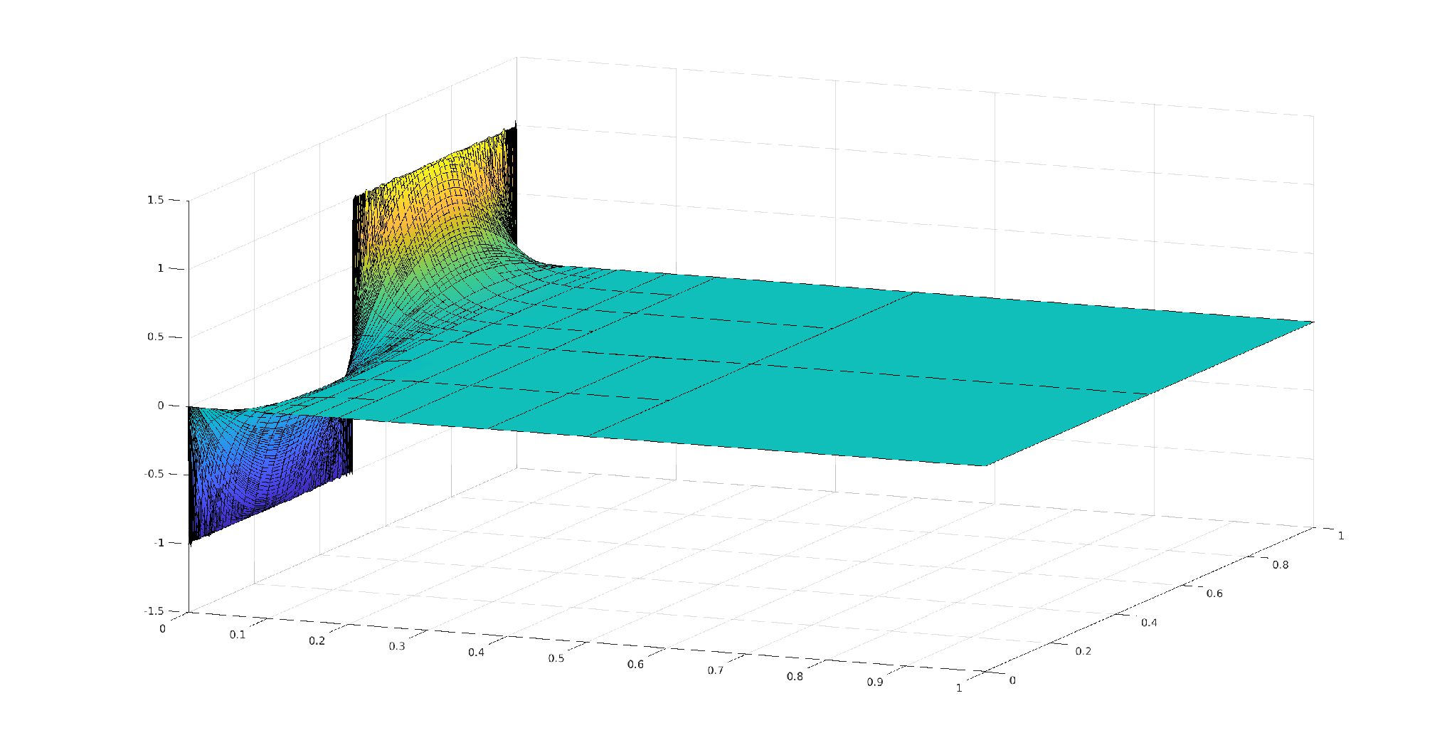
Refer to caption — Figure 3. Solution $\hat{u}_{h}\in V_{h}$ with underlying partition $\mathcal{T}$ and $\textup{ndof}=5385$ as well as the convergence history of the residual $\eta^{2}(\mathcal{T})$ with uniform mesh refinements (solid line) and adaptive mesh refinements (dotted lines) with equally and parabolically scaled mesh refinements for Experiment 3 (Irregular Initial Data).

7.4. Experiment 4 (Rough Right-Hand-Side)

In this experiment the initial data equals $u_{0}=0$ . We investigate our numerical scheme with two singular right-hand sides. They read for all $(t,x)\in Q$ and parameters $\alpha\leq 0$

\displaystyle\begin{aligned} {\mathbf{f}}&=(f_{x}^{\alpha},0)&&\quad\text{with }f_{x}^{\alpha}(t,x)=|x-1/2|^{\alpha},\\ {\mathbf{f}}&=(f_{t}^{\alpha},0)&&\quad\text{with }f_{t}^{\alpha}(t,x)=|t-1/2|^{\alpha}.\end{aligned}

Since the right-hand side satisfies $f\in L^{|1/\alpha|-\varepsilon}(Q)$ , we expect the maximal regularity $\partial_{t}u,\Delta_{x}u\in L^{|1/\alpha|-\varepsilon}(Q)$ for all $\alpha\leq 0$ and $\varepsilon>0$ [Fac17]. Therefore, the estimate in (72) suggest the failure for equally refined meshes as $\alpha\searrow 1/2$ . Table 1 displays the rates of convergence of the squared residual $\lVert(\eta_{h},\vartheta_{h})\rVert_{Y}^{2}$ for various values of $\alpha$ and the right-hand sides $f_{x}^{\alpha}$ (“Singular in Space”) and $f_{t}^{\alpha}$ (“Singular in Time”). We compute the rates via linear regression of the log log convergence history plot, where the number of degrees of freedom on the initial partition $\mathcal{T}$ equals $\textup{ndof}=9$ and is larger than $10^{5}<\textup{ndof}$ on the finest partition. We observe that the singularity causes severe difficulties for equally scaled mesh refinements in the sense that the rate of convergence goes for uniform and adaptive mesh refinements to zero as $\alpha\searrow-1/2$ (the limiting cases for ${\mathbf{f}}\not\in L^{2}(Q;\mathbb{R}^{d+1})$ ). The parabolically scaled scheme works significantly better: the rate of convergence for uniform and adaptive refinements is above $2/3$ for $\alpha\geq-1/2$ , which is the optimal rate for smooth solutions. This underlines the theoretical considerations in Section 6.5. Notice that we have to add the data approximation error (not displayed in this paper) to the residuals in Table 1 to conclude decay rates for the error. For the right-hand side $f_{x}^{\alpha}$ and $\alpha\geq-0.4$ the data approximation error for the parabolically scaled uniform and adaptive refinements converges with a rate faster than $2/3$ , for $\alpha=-0.5$ the rate equals $0.55$ . For the right-hand side $f_{t}^{\alpha}$ the convergence rate of the data approximation error goes to zeros as $\alpha\searrow-1/2$ . Nevertheless, this experiment indicates that parabolically scaled mesh refinements are obligatory for rough solutions.

	Singular in Space				Singular in Time
	Equal		Parabolic		Equal		Parabolic
$\alpha$	unif	adapt	unif	adapt	unif	adapt	unif	adapt
0.00	1	1.01	0.66	0.66	1	1.01	0.66	0.66
-0.05	0.81	0.93	0.67	0.67	0.81	0.93	0.66	0.66
-0.1	0.6	0.83	0.67	0.68	0.59	0.82	0.67	0.65
-0.15	0.46	0.71	0.67	0.7	0.45	0.7	0.67	0.67
-0.2	0.36	0.6	0.68	0.71	0.36	0.59	0.67	0.68
-0.25	0.29	0.49	0.69	0.72	0.28	0.48	0.68	0.69
-0.3	0.22	0.39	0.69	0.75	0.22	0.38	0.69	0.72
-0.35	0.17	0.29	0.69	0.76	0.16	0.28	0.7	0.74
-0.4	0.11	0.19	0.67	0.76	0.11	0.18	0.7	0.77
-0.45	0.06	0.08	0.65	0.76	0.06	0.07	0.69	0.79
-0.5	0	-0.02	0.62	0.76	0	-0.03	0.65	0.81
-0.55	-0.05	-0.12	0.59	0.73	-0.05	-0.12	0.6	0.79
-0.6	-0.1	-0.21	0.55	0.71	-0.1	-0.22	0.53	0.78
-0.65	-0.15	-0.31	0.51	0.68	-0.15	-0.32	0.47	0.64
-0.7	-0.2	-0.41	0.47	0.62	-0.2	-0.4	0.4	0.58
-0.75	-0.25	-0.5	0.43	0.56	-0.25	-0.48	0.33	0.42

Table 1. Convergence rates of the squared residual

\lVert(\eta_{h},\vartheta_{h})\rVert_{Y}^{2}

in Experiment 4 (Rough RHS) for various parameters

\alpha

, equally and parabolicly scaled meshes as well as uniform (unif) and adaptive (adapt) mesh refinements.

References

[ABV13] N. Antonić, K. Burazin, and M. Vrdoljak, Heat equation as a Friedrichs system, J. Math. Anal. Appl. 404 (2013), no. 2, 537–553. MR 3045193
[And13] R. Andreev, Stability of sparse space-time finite element discretizations of linear parabolic evolution equations, IMA J. Numer. Anal. 33 (2013), no. 1, 242–260. MR 3020957
[Bab71] I. M. Babuška, Error-bounds for finite element method, Numer. Math. 16 (1970/71), 322–333.
[BDS18] D. Broersen, W. Dahmen, and R. P. Stevenson, On the stability of DPG formulations of transport equations, Math. Comp. 87 (2018), no. 311, 1051–1082. MR 3766381
[CDG14] C. Carstensen, L. Demkowicz, and J. Gopalakrishnan, A posteriori error control for DPG methods, SIAM J. Numer. Anal. 52 (2014), no. 3, 1335–1353.
[CDG16] by same author, Breaking spaces and forms for the DPG method and applications including Maxwell equations, Comput. Math. Appl. 72 (2016), no. 3, 494–522. MR 3521055
[CGHW14] C. Carstensen, D. Gallistl, F. Hellwig, and L. Weggler, Low-order dPG-FEM for an elliptic PDE, Comput. Math. Appl. 68 (2014), 1503–1512. MR 3279489
[DG10] L. Demkowicz and J. Gopalakrishnan, A class of discontinuous Petrov-Galerkin methods. Part I: The transport equation, Comput. Methods Appl. Mech. Engrg. 199 (2010), 1558–1572. MR 2630162 (2011e:65263)
[DG11] by same author, A class of discontinuous Petrov-Galerkin methods. Part II: Optimal test functions, Numer. Methods Partial Differential Equations 27 (2011), 70–105. MR 2743600 (2011k:65155)
[DGNS17] L. Demkowicz, J. Gopalakrishnan, S. Nagaraj, and P. Sepúlveda, A spacetime DPG method for the Schrödinger equation, SIAM J. Numer. Anal. 55 (2017), no. 4, 1740–1759. MR 3672373
[DL92] R. Dautray and J.-L. Lions, Mathematical analysis and numerical methods for science and technology. Vol. 5, Springer-Verlag, Berlin, 1992, Evolution problems. I, With the collaboration of Michel Artola, Michel Cessenat and Hélène Lanchon. MR 1156075
[DS19] W. Dahmen and R. P. Stevenson, Adaptive strategies for transport equations, Comput. Methods Appl. Math. 19 (2019), no. 3, 431–464. MR 3977482
[DSSV17] L. Diening, S. Schwarzacher, B. Stroffolini, and A. Verde, Parabolic Lipschitz truncation and caloric approximation, Calc. Var. Partial Differential Equations 56 (2017), no. 4, Paper No. 120, 27. MR 3672391
[DST21] L. Diening, J. Storn, and T. Tscherpel, On the Sobolev and ${L}^{p}$ -stability of the ${L}^{2}$ -projection, accepted for publication in SIAM J. Numer. Anal. (2021).
[EDCM14] T. E. Ellis, L. F. Demkowicz, J. L. Chan, and R. D. Moser, Space-time DPG: Designing a method for massively parallel CFD, ICES Report (2014), 14–32.
[EG06] A. Ern and J.-L. Guermond, Discontinuous Galerkin methods for Friedrichs’ systems. I. General theory, SIAM J. Numer. Anal. 44 (2006), no. 2, 753–778. MR 2218968
[Eva10] L. C. Evans, Partial differential equations, second ed., Graduate Studies in Mathematics, vol. 19, American Mathematical Society, Providence, RI, 2010. MR 2597943
[EW19] J. Ernesti and C. Wieners, Space-time discontinuous Petrov-Galerkin methods for linear wave equations in heterogeneous media, Comput. Methods Appl. Math. 19 (2019), no. 3, 465–481. MR 3977483
[Fac17] S. Fackler, J.-L. Lions’ problem concerning maximal regularity of equations governed by non-autonomous forms, Ann. Inst. H. Poincaré Anal. Non Linéaire 34 (2017), no. 3, 699–709. MR 3633741
[FHK21] T. Führer, N. Heuer, and M. Karkulik, Analysis of backward Euler primal DPG methods, arXiv preprint 2103.12181 (2021).
[FHN19] T. Führer, N. Heuer, and A. H. Niemi, An ultraweak formulation of the Kirchhoff-Love plate bending model and DPG approximation, Math. Comp. 88 (2019), no. 318, 1587–1619. MR 3925478
[FHS20] T. Führer, N. Heuer, and F.-J. Sayas, An ultraweak formulation of the Reissner-Mindlin plate bending model and DPG approximation, Numer. Math. 145 (2020), no. 2, 313–344. MR 4107221
[FHSG17] T. Führer, N. Heuer, and J. Sen Gupta, A time-stepping DPG scheme for the heat equation, Comput. Methods Appl. Math. 17 (2017), no. 2, 237–252. MR 3630108
[FK21] T. Führer and M. Karkulik, Space-time least-squares finite elements for parabolic equations, Comput. Math. Appl. 92 (2021), 27–36. MR 4242919
[FS20] S. A. Funken and A. Schmidt, Adaptive mesh refinement in 2D—an efficient implementation in Matlab, Comput. Methods Appl. Math. 20 (2020), no. 3, 459–479. MR 4116623
[GMO14] J. Gopalakrishnan, I. Muga, and N. Olivares, Dispersive and dissipative errors in the DPG method with scaled norms for Helmholtz equation, SIAM J. Sci. Comput. 36 (2014), no. 1, A20–A39. MR 3148088
[GQ14] J. Gopalakrishnan and W. Qiu, An analysis of the practical DPG method, Math. Comp. 83 (2014), no. 286, 537–552. MR 3143683
[GS19] J. Gopalakrishnan and P. Sepúlveda, A space-time DPG method for the wave equation in multiple dimensions, Space-Time Methods, edited by U. Langer and O. Steinbach, Berlin, Boston: De Gruyter (2019), 117–140.
[GS21] G. Gantner and R. Stevenson, Further results on a space-time FOSLS formulation of parabolic PDEs, ESAIM Math. Model. Numer. Anal. 55 (2021), no. 1, 283–299. MR 4216839
[LMN16] U. Langer, S. E. Moore, and M. Neumüller, Space-time isogeometric analysis of parabolic evolution problems, Comput. Methods Appl. Mech. Engrg. 306 (2016), 342–363. MR 3502571
[Moo18] S. E. Moore, A stable space-time finite element method for parabolic evolution problems, Calcolo 55 (2018), no. 2, Paper No. 18, 19. MR 3787872
[PD17] S. Petrides and L. F. Demkowicz, An adaptive DPG method for high frequency time-harmonic wave propagation problems, Comput. Math. Appl. 74 (2017), no. 8, 1999–2017. MR 3715175
[RH20] N. V. Roberts and S. Henneking, Time-stepping dpg formulations for the heat equation, Comput. Math. Appl. (2020).
[SS09] C. Schwab and R. Stevenson, Space-time adaptive wavelet methods for parabolic evolution problems, Math. Comp. 78 (2009), no. 267, 1293–1318. MR 2501051
[Ste15] O. Steinbach, Space-time finite element methods for parabolic problems, Comput. Methods Appl. Math. 15 (2015), no. 4, 551–566. MR 3403450
[Sto19] J. Storn, Topics in least-squares and discontinuous Petrov-Galerkin finite element analysis, Doctoral thesis, Humboldt-Universität zu Berlin, 2019.
[Sto20] by same author, On a relation of discontinuous Petrov-Galerkin and least-squares finite element methods, Comput. Math. Appl. 79 (2020), no. 12, 3588–3611. MR 4094782
[SW21] R. Stevenson and J. Westerdiep, Stability of Galerkin discretizations of a mixed space-time variational formulation of parabolic evolution equations, IMA J. Numer. Anal. 41 (2021), no. 1, 28–47. MR 4205051
[Wie16] C. Wieners, The skeleton reduction for finite element substructuring methods, Numerical mathematics and advanced applications—ENUMATH 2015, Lect. Notes Comput. Sci. Eng., vol. 112, Springer, [Cham], 2016, pp. 133–141. MR 3706362

A Space-Time DPG Method for the Heat EquationThanks: This research was supported by the DFG through the CRC 1283 “Taming uncertainty and profiting from randomness and low regularity in analysis, stochastics and their applications”

Abstract.

Key words and phrases:

2020 Mathematics Subject Classification

1. Introduction

2. Heat Equation

Lemma 1 (Relation to Bochner spaces).

Lemma 2 (Control of time derivative).

Proof.

Theorem 3 (Equivalence of norms).

Proof.

Remark 4 (Dependence on TendT_{\textup{end}}).

Lemma 5 (Alternative characterizations of U0U_{0}).

Proof.

Lemma 6 (Dense subspace).

Proof.

Lemma 7 (Alternative characterization of U00U_{00}).

Proof.

3. Design of the DPG Method

Definition 8 (Variational formulation).

Lemma 9 (Unbroken functions).

Proof.

Lemma 10 (Identical traces).

Proof.

Theorem 11 (Equivalent problems).

Proof.

4. Analysis of the Variational Problem

Remark 12 (Trial-to-test operator).

Theorem 13 (Extension operator).

Proof.

Remark 14 (Norms).

Remark 15 (Duality lemma).

Lemma 16 (Inf-sup constant).

Proof.

Theorem 17 (Well-posedness).

Proof.

Remark 18 (Optimal weight).

5. Abstract Discretized Problem

Lemma 19 (Equivalence).

Proof.

6. Practical DPG Scheme

6.1. Partition

6.2. Discretization

Remark 20 (Skeleton reduction/Static condensation).

6.3. Fortin Operator

Theorem 21 (Fortin operator Π\Pi).

Lemma 22 (Local Fortin operator ΠK\Pi_{K}).

Lemma 23 (Auxiliary result).

Proof.

Proof of Lemma 22.

6.4. Error Control

Lemma 24 (Interpolation on tensor product meshes).

Proof.

Lemma 25 (Properties of the time average 𝒫ℙ0​L2\mathcal{P}_{\mathbb{P}_{0}L^{2}}).

Proof.

Theorem 26 (Data Approximation).

Proof.

6.5. Equal vs. Parabolic Scaling

Lemma 27 (Parabolic Poincaré).

Proof.

7. Numerical Experiments

7.1. Experiment 1 (Known Solution)

7.2. Experiment 2 (Checkerboard)

7.3. Experiment 3 (Irregular Initial Data)

7.4. Experiment 4 (Rough Right-Hand-Side)

References

Remark 4 (Dependence on $T_{\textup{end}}$ ).

Lemma 5 (Alternative characterizations of $U_{0}$ ).

Lemma 7 (Alternative characterization of $U_{00}$ ).

Theorem 21 (Fortin operator $\Pi$ ).

Lemma 22 (Local Fortin operator $\Pi_{K}$ ).

Lemma 25 (Properties of the time average $\mathcal{P}_{\mathbb{P}_{0}L^{2}}$ ).