跳到论文正文
W Papers独立论文阅读器 arXiv:2012.13187 论文正文 计算阅读时间 · 0%
引用这篇论文根据当前论文元数据生成,正式投稿前建议核对。


License: CC BY-SA 4.0
arXiv:2012.13187v3 [physics.class-ph] 04 Sep 2023

A Shell Frictionally Coupled to an Elastic Foundation and a Comparison Against the Two-Body Coulomb’s Law of Static Friction Note: This work is based on a PhD thesis submitted to UCL in 2016 [3], and the initial research was funded by The Dunhill Medical Trust [grant number R204/0511] and UCL Impact Studentship.

Kavinda Jayawardana Email: kavjayawardana@tekoptimaresearch.com; zcahe58@ucl.ac.uk Address: TEK Optima Research Ltd, Unit 10 Westcroft Buiness Park Oakdene Drive, Three Legged Cross, Wimborne BH21 6FQ Corresponding author: Corresponding author
Abstract

In this article, we derive a model for a shell that is frictionally coupled to an elastic foundation. We use Kikuchi and Oden’s model for Coulomb’s law of static friction [1] to derive a displacement-based static-friction law for a shell on an elastic foundation model, and we prove the existence and the uniqueness of solutions with the aid of the work of Kinderlehrer and Stampacchia [2]. For numerical analysis, we modify Kikuchi and Oden’s model for Coulomb’s law of static friction [1] to model a full two-body contact problem in curvilinear coordinates. Our numerical results indicate that if the shell has a relatively high Young’s modulus or has a relatively high Poisson’s ratio, and the contact region has a high coefficient of friction or has a high radius of curvature, then the displacement field of the foundation predicted by both models are in better agreement. As far as we are aware, this is the first derivation of a displacement-based friction law and a two-body 3D elasticity contact problem with friction in the literature.

Keywords: 
Contact Mechanics , Coulomb’s Law of Static Friction , Curvilinear Coordinates , Elastic Foundations, Mathematical Elasticity , Shell Theory
2010 MSC
74M10 , 74K25 , 74B05

1 Introduction

Consider a situation where two elastic bodies are in contact with each other and the contact region exhibits friction, where friction defined as the force that oppose potential relative motion between the two bodies. A common area where modelling of such problems can be found is in the field of tyre manufacturing [4, 5]. Assume now where one of the elastic bodies is very thin and almost planar in a curvilinear sense relative to the other body. Then the thin body can be approximated by a shell or a membrane, and such models can be used to model skin abrasion caused by fabrics as a result of friction [6]. There is a need for valid modelling techniques in fields such as sports related skin trauma [7] and cosmetics [8]. It is documented that abrasion damage to human skin in cases such as the jogger’s nipple [9] and dermatitis from clothing [10] are caused by repetitive movement of fabrics on skin, and in cases such as pressure ulcers [11] and juvenile plantar dermatitis [12], friction may worsen the problem. The aim of this article is to present a simple but a mathematically valid method to model such problems, i.e. a mathematical model for a shell on an elastic foundation when subjected to a displacement-based friction condition in a static dry-friction (see section 11.3 of Kikuchi and Oden [1]) setting.

1.1 Modelling Difficulties

Consider a three-dimensional elastic body that is in contact with a rigid boundary whose contact area is rough, i.e. contact area exhibits friction (see chapter 13 of Johnson [13] or section 5.2 of Quadling and Neill [14]), then, given that we know the pressure experienced on the elastic body at the contact region in advance, the governing equations that describe the behaviour at the contact region can be represented by Kikuchi and Oden’s model for Coulomb’s law of static friction [1], which has the following formulation in Euclidean coordinates

jε(u)={∫Γ[𝒦​|uT|−12​ε]​ds,if​|uT|≥ε,∫Γ[12​𝒦​|uT|2ε]​ds,if​|uT|<ε,\qquad j_{\varepsilon}(\textbf{u})=\left\{\begin{aligned} \int_{\Gamma}\left[\mathscr{K}|\textbf{u}_{T}|-\frac{1}{2}\varepsilon\right]ds,~&\text{if}~|\textbf{u}_{T}|\geq\varepsilon,\\ \int_{\Gamma}\left[\frac{1}{2}\mathscr{K}\frac{|\textbf{u}_{T}|^{2}}{\varepsilon}\right]ds,~&\text{if}~|\textbf{u}_{T}|<\varepsilon,\end{aligned}\right. (1)

where νF\nu_{F} is the coefficient of friction, u is the displacement field and uT\textbf{u}_{T} is the tangential displacement field of the contact boundary, 𝒦\mathscr{K} (units: Nm−2\text{Nm}^{-2}) is the spring modulus, ε\varepsilon is the regularisation parameter, and Γ\Gamma is the contact region between elastic body and rigid obstacle. Let 𝝈T​(u)\boldsymbol{\sigma}_{T}(\textbf{u}) and σn​(u)\sigma_{n}(\textbf{u}) be the normal-tangential stress and purely-normal stress tensors at the contact boundary respectively. Thus, if one assumes that the purely-normal stress, σn​(u)<0\sigma_{n}(\textbf{u})<0 (i.e. pressure), is no longer an unknown, but it is prescribed, and further assumes that 𝒦=−νF​σn​(u)\mathscr{K}=-\nu_{F}\sigma_{n}(\textbf{u}), then the Gâteaux derivative (see definition 1.3.7 of Badiale and Serra [15]) of jε​(⋅)j_{\varepsilon}(\cdot) has the following form

𝝈T(u)={νF​σn​(u)​uT|uT|,if​|uT|≥ε,νF​σn​(u)​uTε,if​|uT|<ε.\qquad\boldsymbol{\sigma}_{T}(\textbf{u})=\left\{\begin{aligned} \nu_{F}\sigma_{n}(\textbf{u})\frac{\textbf{u}_{T}}{|\textbf{u}_{T}|},&~\text{if}~|\textbf{u}_{T}|\geq\varepsilon,\\ \nu_{F}\sigma_{n}(\textbf{u})\frac{\textbf{u}_{T}}{\varepsilon},&~\text{if}~|\textbf{u}_{T}|<\varepsilon.\end{aligned}\right. (2)

Now, assume that we are considering a shell (i.e. two-dimensional representation of a very thin three-dimensional elastic body), then the very idea of normal stress becomes meaningless. This is because for a shell, we find that σT​(u)=𝟎\sigma_{T}(\textbf{u})=\boldsymbol{0} and σn​(u)=0\sigma_{n}(\textbf{u})=0, and thus, Kikuchi and Oden’s model [1], i.e. equation (2), will fail to be applicable. Note that for a thorough mathematical analysis of the shell theory, consult chapter 4 of Ciarlet [16].

One could find other 1D and 2D-elasticity models that incorporates friction, such as the capstan equation, belt-friction models [17], and beams with friction [18]; however, all such models (including Kikuchi and Oden’s model [1]) deal with a rigid obstacle as the contact surface, and thus, at the presence of an elastic obstacle (i.e. a two-body elasticity contact problem with friction), all such friction models fail. Currently, there exist two-body 1D-elasticity contact models with friction in the literature (i.e. analysis of elastic strings in contact [19, 20, 21, 22]). However, the literature still lacks two-body 2D and 3D-elasticity contact models with friction.

2 A Shell Frictionally Coupled to an Elastic Foundation

Refer to caption
Figure 1: Schematic representation of a shell frictionally coupled to an elastic foundation in Euclidean space, where hh is the thickness and τ0\tau_{\!0} is some traction acting on the boundary of the shell

In this section, we modify Kikuchi and Oden’s model for Coulomb’s law of static friction [1] to derive a friction condition to model the behaviour of an elastic shell that is frictionally coupled to an elastic-foundation (see fig. 1). To do so, consider an unstrained static three-dimensional isotropic elastic body (which we call the foundation) whose volume is described by the diffeomorphism 𝑿¯∈C2​(Ω¯CLOSE;\bar{\boldsymbol{X}}\in C^{2}(\bar{\Omega}; OPENE3)\textbf{E}^{3}), where Ω⊂ℝ3\Omega\subset\mathbb{R}^{3} is a connected open bounded domain that satisfies the segment condition with a uniform-C1​(ℝ3,ℝ2)C^{1}(\mathbb{R}^{3};\mathbb{R}^{2}) boundary (see definition 4.10 of Adams and Fournier [23]), Ck​(⋅)C^{k}(\cdot) is a space of continuous functions that has continuous first kk partial derivatives in the underlying domain, Ek\textbf{E}^{k} is the kk-dimensional Euclidean space and ℝk\mathbb{R}^{k} is the kk-dimensional curvilinear space. Now, assume that there exists a thinner isotropic elastic body (which we call the shell, i.e. a planar elastic body with constant thickness hh whose rest configuration is curvilinear) frictionally coupled to a subset of the boundary of the foundation such that the contact region is initially stress-free, where this contact region is described by the injection 𝝈∈C3​(ω¯,E2)\boldsymbol{\sigma}\in C^{3}(\bar{\omega};\textbf{E}^{2}) and where ω⊂ℝ2\omega\subset\mathbb{R}^{2} is a connected open bounded plane that satisfies the segment condition with a uniform-C1​(ℝ2,ℝ)C^{1}(\mathbb{R}^{2};\mathbb{R}) boundary. Note that in our analysis, we only consider shells that satisfy the following condition:

Condition 1.

Let the map 𝛔∈C3​(ω¯,E2)\boldsymbol{\sigma}\in C^{3}(\bar{\omega};\textbf{E}^{2}) describes the lower-surface of an unstrained shell, where ω⊂ℝ2\omega\subset\mathbb{R}^{2} is a connected open bounded plane that satisfies the segment condition with a uniform-C1​(ℝ2,ℝ)C^{1}(\mathbb{R}^{2};\mathbb{R}) boundary. Given that the thickness of the shell is hh, we require the following condition to be satisfied

0≤h2​K<h​H≪1,∀(x1,x2)∈ω¯,\displaystyle 0\leq h^{2}K<hH\ll 1,~\forall~\boldsymbol{(}x^{1},x^{2}\boldsymbol{)}\in\bar{\omega},

where KK is the Gaussian curvature and HH is the mean curvature, i.e. the lower-surface of the shell is non-hyperbolic and it is a surface with a positive mean curvature, and the thickness of the shell is sufficiently small.

Note that K=(F[II]​11​F[II]​22−F[II]​12​F[II]​21)K=(F_{\!\text{[II]}1}^{~~1}F_{\!\text{[II]}2}^{~~2}-F_{\!\text{[II]}1}^{~~2}F_{\!\text{[II]}2}^{~~1}), H=−12​F[II]​ααH=-\frac{1}{2}F_{\!\text{[II]}\alpha}^{~~\alpha},

F[II]​α​β=𝑵⋅∂α​β𝝈,α,β∈{1,2},\displaystyle F_{\!\text{[II]}\alpha\beta}=\boldsymbol{N}\cdot\partial_{\alpha\beta}\boldsymbol{\sigma},~~\alpha,\beta\in\{1,2\},

is the second fundamental form tensor of 𝝈\boldsymbol{\sigma},

𝑵=∂1𝝈×∂2𝝈‖∂1𝝈×∂2𝝈‖\displaystyle\boldsymbol{N}=\frac{\partial_{1}\boldsymbol{\sigma}\times\partial_{2}\boldsymbol{\sigma}}{||\partial_{1}\boldsymbol{\sigma}\times\partial_{2}\boldsymbol{\sigma}||}

is the unit normal to the surface 𝝈\boldsymbol{\sigma}, ∂α\partial_{\alpha} are partial derivatives with respect to curvilinear coordinates xαx^{\alpha}, and ⋅\cdot, ×\times and ||⋅||||\cdot|| are the Euclidean dot product, the Euclidean cross product and the Euclidean norm respectively. Also, note that Einstein’s summation notation (see section 1.2 of Kay [24]) is assumed throughout, bold symbols signify that we are dealing with vector and tensor fields, we regard the indices i,j,k,l∈{1,2,3}i,j,k,l\in\{1,2,3\} and α,β,γ,δ∈{1,2}\alpha,\beta,\gamma,\delta\in\{1,2\}, and we usually reserve the vector brackets (⋅)E\boldsymbol{(}\cdot\boldsymbol{)}_{\text{E}} for vectors in the Euclidean space and (⋅)\boldsymbol{(}\cdot\boldsymbol{)} for vectors in the curvilinear space.

With condition 1 and in accordance with the work of Jayawardana [3], we can express the energy functional of a shell bonded to an elastic foundation as follows

J⁡(𝒖)=\displaystyle J(\boldsymbol{u})= ∫Ω[12​Ai​j​k​l​Ei​j​(𝒖)​Ek​l​(𝒖)−fi​ui]​𝑑Ω\displaystyle\int_{\Omega}\left[\frac{1}{2}A^{ijkl}E_{ij}(\boldsymbol{u})E_{kl}(\boldsymbol{u})-f^{i}u_{i}\right]d\Omega
+∫ω[12Bα​β​γ​δ(hϵα​β(𝒖)ϵγ​δ(𝒖)+13h3ρα​β(𝒖)ργ​δ(𝒖))−hf0iui]dω\displaystyle+\int_{\omega}\bigg[\frac{1}{2}B^{\alpha\beta\gamma\delta}\bigg(h\epsilon_{\alpha\beta}(\boldsymbol{u})\epsilon_{\gamma\delta}(\boldsymbol{u})+\frac{1}{3}h^{3}\rho_{\alpha\beta}(\boldsymbol{u})\rho_{\gamma\delta}(\boldsymbol{u})\bigg)-hf_{0}^{i}u_{i}\bigg]d\omega
−∫∂ωhτ0iuid(∂ω),\displaystyle-\int_{\partial\omega}h\tau_{\!0}^{i}u_{i}~d(\partial\omega),

where 𝒖\boldsymbol{u} is the displacement field, Ti​j​(𝒖)=Ai​j​k​l​Ek​l​(𝒖)T^{ij}(\boldsymbol{u})=A^{ijkl}E_{kl}(\boldsymbol{u}) is second Piola-Kirchhoff stress tensor of the foundation, Ei​j​(𝒖)=12​(∇¯i​uj+∇¯j​uj)E_{ij}(\boldsymbol{u})=\frac{1}{2}(\bar{\nabla}_{\!i}u_{j}+\bar{\nabla}_{\!j}u_{j}) is linearised Green-St Venant strain tensor of the foundation,

Ai​j​k​l=λ¯​gi​j​gk​l+μ¯​(gi​k​gj​l+gi​l​gj​k)A^{ijkl}=\bar{\lambda}g^{ij}g^{kl}+\bar{\mu}(g^{ik}g^{jl}+g^{il}g^{jk})

is the isotropic elasticity tensor of the foundation,

gi​j=∂i𝑿¯⋅∂j𝑿¯,i,j∈{1,2,3},\displaystyle g_{ij}=\partial_{i}\bar{\boldsymbol{X}}\cdot\partial_{j}\bar{\boldsymbol{X}},~i,j\in\{1,2,3\},

is the covariant metric tensor of 𝑿¯\bar{\boldsymbol{X}}, ∂j\partial_{j} is the partial derivative with respect to the coordinate xjx^{j},

λ¯=ν¯​E¯(1+ν¯)​(1−2​ν¯)\bar{\lambda}=\frac{\bar{\nu}\bar{E}}{(1+\bar{\nu})(1-2\bar{\nu})}

and

μ¯=12​E¯1+ν¯\bar{\mu}=\frac{1}{2}\frac{\bar{E}}{1+\bar{\nu}}

are the first and the second Lamé’s parameters of the foundation respectively, E¯∈(0,∞)\bar{E}\in(0,\infty) is the Young’s modulus of the foundation and ν¯∈(−1,12)\bar{\nu}\in(-1,\frac{1}{2}) is the Poisson’s ratio of the elastic foundation, 𝒇\boldsymbol{f} is an external force density field acting on the elastic foundation, and 𝒏¯\bar{\boldsymbol{n}} is the unit outward normal to the boundary ∂Ω\partial\Omega in curvilinear coordinates. Furthermore, τα​β​(𝒖)=Bα​β​γ​δ​ϵγ​δ​(𝒖)\tau^{\alpha\beta}(\boldsymbol{u})=B^{\alpha\beta\gamma\delta}\epsilon_{\gamma\delta}(\boldsymbol{u}) is the stress tensor, ηα​β​(𝒖)=Bα​β​γ​δ​ργ​δ​(𝒖)\eta^{\alpha\beta}(\boldsymbol{u})=B^{\alpha\beta\gamma\delta}\rho_{\gamma\delta}(\boldsymbol{u}) negative of the change in moments density tensor of the shell,

ϵα​β​(𝒖)=[12​(∇αuβ+∇βuα)−g3​F[II]​α​β​u3]|ω\displaystyle\epsilon_{\alpha\beta}(\boldsymbol{u})=\left[\frac{1}{2}\left(\nabla_{\!\alpha}u_{\beta}+\nabla_{\!\beta}u_{\alpha}\right)-g_{3}F_{\!\text{[II]}\alpha\beta}u^{3}\right]\!|_{\omega}

is half of the change in the first fundamental form tensor of the shell and g3=g33|ω=1g_{3}=\sqrt{g_{33}}|_{\omega}=1 by construction,

ρα​β(𝒖)=[g3(∇α∇βu3−F[II]​α​γF[II]​βγu3)+F[II]​β​γ∇αuγ\displaystyle\rho_{\alpha\beta}(\boldsymbol{u})=\Big[g_{3}\left(\nabla_{\!\alpha}\nabla_{\!\beta}u^{3}-F_{\!\text{[II]}\alpha\gamma}F_{\!\text{[II]}\beta}^{~~\gamma}u^{3}\right)+F_{\!\text{[II]}\beta\gamma}\nabla_{\!\alpha}u^{\gamma}
+F[II]​α​γ​∇βuγ+(∇αF[II]​β​γ)​uγ\displaystyle+F_{\!\text{[II]}\alpha\gamma}\nabla_{\!\beta}u^{\gamma}+\left(\nabla_{\!\alpha}F_{\!\text{[II]}\beta\gamma}\right)u^{\gamma} ]|ω\displaystyle\Big]|_{\omega}

the change in the second fundamental form tensor of the shell,

Bα​β​γ​δ\displaystyle B^{\alpha\beta\gamma\delta} =2​λ​μλ+2​μ​F[I]α​β​F[I]γ​δ+μ⁡(F[I]α​γ​F[I]β​δ+F[I]α​δ​F[I]β​γ)\displaystyle=\frac{2\lambda\mu}{\lambda+2\mu}F_{\!\text{[I]}}^{\alpha\beta}F_{\!\text{[I]}}^{\gamma\delta}+\mu(F_{\!\text{[I]}}^{\alpha\gamma}F_{\!\text{[I]}}^{\beta\delta}+F_{\!\text{[I]}}^{\alpha\delta}F_{\!\text{[I]}}^{\beta\gamma})

is the isotropic elasticity tensor of the shell,

λ=ν​E(1+ν)​(1−2​ν)\lambda=\frac{\nu E}{(1+\nu)(1-2\nu)}

and

μ=12​E1+ν\mu=\frac{1}{2}\frac{E}{1+\nu}

are the first and the second Lamé’s parameters of the shell respectively, E∈(0,∞)E\in(0,\infty) is the Young’s modulus of the shell and ν∈(−1,12)\nu\in(-1,\frac{1}{2}) is the Poisson’s ratio of the shell, 𝒇0\boldsymbol{f}_{0} is an external force density field acting on the shell, 𝒏\boldsymbol{n} is the unit outward normal vector to the boundary ∂ω\partial\omega in curvilinear coordinates, 𝝉0\boldsymbol{\tau}_{\!0} is an external traction field acting on the boundary of the shell, and 𝒖|ω\boldsymbol{u}|_{\omega} is in a trace sense (see section 5.5 of Evans [25]). Finally, ∇¯\bar{\boldsymbol{\nabla}} is the covariant derivative operator in the curvilinear space, i.e. for any 𝒗∈C1​(Ω¯,ℝ3)\boldsymbol{v}\in C^{1}(\bar{\Omega};\mathbb{R}^{3}), we define its covariant derivative as follows

∇¯j​vk=∂jvk+Γ¯i​jk​vi,\displaystyle\bar{\nabla}_{\!j}v^{k}=\partial_{j}v^{k}+\bar{\Gamma}^{k}_{\!ij}v^{i},

where

Γ¯i​jk=12gk​l(−∂lgi​j+∂igj​l+∂jgl​i)\displaystyle\bar{\Gamma}^{k}_{\!ij}=\frac{1}{2}g^{kl}\left(-\partial_{l}g_{ij}+\partial_{i}g_{jl}+\partial_{j}g_{li}\right)

are the Christoffel symbols of the second kind, and ∇\boldsymbol{\nabla} is the covariant derivative operator in the curvilinear plane, i.e. for any 𝒖∈C1​(ω¯,ℝ2)\boldsymbol{u}\in C^{1}(\bar{\omega};\mathbb{R}^{2}), we define its covariant derivative as follows

∇βuγ=∂βuγ+Γα​βγ​uα,\displaystyle\nabla_{\!\beta}u^{\gamma}=\partial_{\beta}u^{\gamma}+\Gamma^{\gamma}_{\!\alpha\beta}u^{\alpha},

where

Γα​βγ=12F[I]γ​δ(−∂δF[I]​α​β+∂αF[I]​β​δ+∂βF[I]​δ​α)\displaystyle\Gamma^{\gamma}_{\!\alpha\beta}=\frac{1}{2}F_{\!\text{[I]}}^{\gamma\delta}\left(-\partial_{\delta}F_{\!\text{[I]}\alpha\beta}+\partial_{\alpha}F_{\!\text{[I]}\beta\delta}+\partial_{\beta}F_{\!\text{[I]}\delta\alpha}\right)

are the Christoffel symbols of the second kind in the curvilinear plane.

Refer to caption
Figure 2: Schematic representation of a two-body problem in curvilinear space: a shell (upper body) on an elastic foundation (middle body), before and after deformation

Now assume that the shell is coupled to the elastic foundation with friction, where a portion of the foundation is satisfying the zero-Dirichlet boundary condition (i.e. clamped). Also, assume that one is applying forces to both the top and to a portion of the boundary of the shell to mimic compression and shear at the contact region respectively (see Fig. 2). Now, if the higher the compression, then the higher the normal displacement towards the bottom, i.e. u3|ω+<0u^{3}|_{\omega^{+}}<0 (condition 1 can guarantee this for sensible boundary tractions), and if the higher the shear, then the higher the tangential displacement in the direction of the applied tangential shear, i.e. (uα​uα)12|ω+>0\left(u_{\alpha}u^{\alpha}\right)^{\frac{1}{2}}|_{\omega^{+}}>0, where ω+=limx3→0+{ω×[0,h)}\omega^{+}=\lim_{x^{3}\to 0^{+}}\{\omega\times[0,h)\} and by convention (uα​uα)12=u1​u1+u2​u2\left(u_{\alpha}u^{\alpha}\right)^{\frac{1}{2}}=\sqrt{u_{1}u^{1}+u_{2}u^{2}}. Now, we consider Kikuchi and Oden’s model for Coulomb’s law of static friction [1] for a thin three-dimensional elastic body (i.e. prior to approximating the thin body with a shell), and once extended to curvilinear coordinates and after taking the limit ε→0\varepsilon\to 0, we find the following

[T3β​(𝒗)+νF​g3​(vα​vα)−12​vβ​T33​(𝒗)]|ω+≤0,\displaystyle\left[T^{\beta}_{3}(\boldsymbol{v})+\nu_{F}g_{3}(v_{\alpha}v^{\alpha})^{-\frac{1}{2}}v^{\beta}T_{3}^{3}(\boldsymbol{v})\right]\!|_{\omega^{+}}\leq 0, (3)

for T33​(𝒗)|∂ω+<0T_{3}^{3}(\boldsymbol{v})|_{\partial\omega^{+}}<0, where 𝒗\boldsymbol{v} is the displacement field and the volume {ω×[0,h]}\{\omega\times[0,h]\} describes the reference configuration of this elastic body. Just as it is for Coulomb’s friction case (where the bodies are in relative equilibrium given that the magnitude of the normal stress is above a certain factor of the magnitude of the tangential stress), we assume that the bodies (i.e. the thin body and the foundation) are in relative equilibrium given that the normal displacement is a below a certain factor of the magnitude of the tangential displacement, i.e.

[(uα​uα)12+C​g3​u3]|ω+≤0,\displaystyle\left[\left(u_{\alpha}u^{\alpha}\right)^{\frac{1}{2}}+Cg_{3}u^{3}\right]\!|_{\omega^{+}}\leq 0, (4)

if u3|ω+≤0u^{3}|_{\omega^{+}}\leq 0, for some dimensionless constant CC. To determine the constant CC, we consider Coulomb’s law of static friction for the limiting equilibrium case (i.e. at the point of slipping) and rearrange equation (3) to obtain the following

[∇¯3((vαvα)12+2νF(1+γ1−2​γ)g3v3)+(2​νF​γ1−2​γ)g3∇¯αvα\displaystyle\bigg[\bar{\nabla}_{\!3}\left((v_{\alpha}v^{\alpha})^{\frac{1}{2}}+2\nu_{F}\left(1+\frac{\gamma}{1-2\gamma}\right)g_{3}v^{3}\right)+\left(\frac{2\nu_{F}\gamma}{1-2\gamma}\right)g_{3}\bar{\nabla}_{\!\alpha}v^{\alpha}
+vδ​∇¯δ​v3(vα​vα)12\displaystyle+\frac{v^{\delta}\bar{\nabla}_{\!\delta}v_{3}}{(v_{\alpha}v^{\alpha})^{\frac{1}{2}}} ]|ω+=0.\displaystyle\bigg]|_{\omega^{+}}=0.

Now, the above equation must hold for all elastic conditions, even under extreme conditions such as the incompressible elasticity condition, i.e. (γ1−2​γ)​∇¯i​vi(\frac{\gamma}{1-2\gamma})\bar{\nabla}_{\!i}v^{i} =p⁡(x1,x2,x3)=p(x^{1},x^{2},x^{3}), where p⁡(⋅)p(\cdot) is a finite function. Thus, we may assume the following equation

[∇¯3((vαvα)12+2νFg3v3)+vδ​∇¯δ​v3(vα​vα)12+2νFg3p(x1,x2,x3)\displaystyle\bigg[\bar{\nabla}_{\!3}\left((v_{\alpha}v^{\alpha})^{\frac{1}{2}}+2\nu_{F}g_{3}v^{3}\right)+\frac{v^{\delta}\bar{\nabla}_{\!\delta}v_{3}}{(v_{\alpha}v^{\alpha})^{\frac{1}{2}}}+2\nu_{F}g_{3}p(x^{1},x^{2},x^{3}) ]|ω+=0.\displaystyle\bigg]|_{\omega^{+}}=0.

Now, nondimensionalise the above equation by making the transformations vi=ℓ​wiv^{i}=\ell w^{i}, xα=ℓ​yαx^{\alpha}=\ell y^{\alpha} and x3=h​y3x^{3}=hy^{3} where ℓ=meas⁡(𝝈⁡(ω),E2)\ell=\sqrt{\mathrm{meas}(\boldsymbol{\sigma}(\omega);\textbf{E}^{2})}, and where meas⁡(⋅,ℝk)\mathrm{meas}(\cdot;\mathbb{R}^{k}) is standard Lebesgue measure in ℝk\mathbb{R}^{k} (see chapter 6 of Schilling [26]), to obtain the following

[(ℓh)\displaystyle\bigg[\left(\frac{\ell}{h}\right) g3​∂∂y3​((wα​wα)12+2​νF​g3​w3)\displaystyle g^{3}\frac{\partial}{\partial y^{3}}\left((w_{\alpha}w^{\alpha})^{\frac{1}{2}}+2\nu_{F}g_{3}w^{3}\right)
+g3​wδ(wα​wα)12(∂w3∂yδ+Γδ​i3wi)+2νFp(ℓy1,ℓy2,hy3)]|ω+=0\displaystyle+\frac{g_{3}w^{\delta}}{(w_{\alpha}w^{\alpha})^{\frac{1}{2}}}\left(\frac{\partial w^{3}}{\partial y^{\delta}}+\Gamma^{3}_{\!\delta i}w^{i}\right)+2\nu_{F}p(\ell y^{1},\ell y^{2},hy^{3})\bigg]|_{\omega^{+}}=0 (5)

where g3=g33|ω=1g^{3}=\sqrt{g^{33}}|_{\omega}=1 by construction. As our goal is to study shells, we consider the limit (h/ℓ)→0(h/\ell)\to 0. As we also require Coulomb’s law of static friction for the limiting-equilibrium case to stay finite in this limit, equation (5) implies that

[(wα​wα)12+2​νF​g3​w3]|{(ωℓ2)×[0,1]}=q⁡(y1,y2)+𝒪⁡((hℓ),y3),\displaystyle\left[(w_{\alpha}w^{\alpha})^{\frac{1}{2}}+2\nu_{F}g_{3}w^{3}\right]\!|_{\{\left(\frac{\omega}{\ell^{2}}\right)\times[0,1]\}}=q(y^{1},y^{2})+\mathcal{O}\left(\left(\frac{h}{\ell}\right),y^{3}\right),

where q⁡(⋅)q(\cdot) is a finite function. As the above equation must hold true when the bodies are deformation free, we find that q⁡(⋅)=0q(\cdot)=0. Furthermore, as we are seeking for a relation of the form of equation (4), we may assume that C=2​νFC=2\nu_{F} is a good approximation. Finally, assuming that 𝒖\boldsymbol{u} is continuous on Ω¯\bar{\Omega}, we arrive at the following hypothesis:

Hypothesis 1.

A shell supported by an elastic foundation with a rough contact area that is in agreement with condition 1 satisfies the following displacement-based friction condition

[2​νF​g3​u3+(uα​uα)12]|ω≤0,\displaystyle\left[2\nu_{F}g_{3}u^{3}+\left(u_{\alpha}u^{\alpha}\right)^{\frac{1}{2}}\right]\!|_{\omega}\leq 0,

where νF\nu_{F} is the coefficient of friction between the shell and the foundation, and 𝐮\boldsymbol{u} is the displacement field of the shell with respect to the contact region ω\omega. If [2​νF​g3​u3+(uα​uα)12]|ω<0[2\nu_{F}g_{3}u^{3}+\left(u_{\alpha}u^{\alpha}\right)^{\frac{1}{2}}]|_{\omega}<0, then we say that the shell is bonded to the foundation, and if [2​νF​g3​u3+(uα​uα)12]|ω=0[2\nu_{F}g_{3}u^{3}+\left(u_{\alpha}u^{\alpha}\right)^{\frac{1}{2}}]|_{\omega}=0, then we say that the shell is at limiting-equilibrium.

Using hypothesis 1, we can now express the energy functional of a shell on a elastic foundation subject to the displacement-based friction condition, and thus, we obtain the following:

Theorem 1.

Let Ω⊂ℝ3\Omega\subset\mathbb{R}^{3} be a connected open bounded domain that satisfies the segment condition with a uniform-C1​(ℝ3,ℝ2)C^{1}(\mathbb{R}^{3};\mathbb{R}^{2}) boundary ∂Ω\partial\Omega such that ω,∂Ω0⊂∂Ω\omega,\partial\Omega_{0}\subset\partial\Omega with ω¯∩∂Ω0¯=Ø\bar{\omega}\cap\bar{\partial\Omega_{0}}={\O} and meas⁡(∂Ω0,ℝ2)>0\mathrm{meas}(\partial\Omega_{0};\mathbb{R}^{2})>0, and let ω⊂ℝ2\omega\subset\mathbb{R}^{2} be a connected open bounded plane that satisfies the segment condition with a uniform-C1​(ℝ2,ℝ)C^{1}(\mathbb{R}^{2};\mathbb{R}) boundary ∂ω\partial\omega. Also, let 𝐗¯∈C2​(Ω¯,E3)\bar{\boldsymbol{X}}\in C^{2}(\bar{\Omega};\textbf{E}^{3}) be a diffeomorphism and 𝛔∈C3​(ω¯,E3)\boldsymbol{\sigma}\in C^{3}(\bar{\omega};\textbf{E}^{3}) be an injective immersion satisfying 0≤h2​K<h​H≪10\leq h^{2}K<hH\ll 1 in ω\omega. Furthermore, let 𝐟∈𝐋2​(Ω)\boldsymbol{f}\in\boldsymbol{L}^{2}(\Omega), 𝐟0∈𝐋2​(ω)\boldsymbol{f}_{\!0}\in\boldsymbol{L}^{2}(\omega) (where f03≤0​a.e.f_{\!0}^{3}\leq 0~\mathrm{a.e.}) and 𝛕0∈𝐋2​(∂ω)\boldsymbol{\tau}_{\!0}\in\boldsymbol{L}^{2}(\partial\omega) (where τ03≤0​a.e.\tau_{\!0}^{3}\leq 0~\mathrm{a.e.}). Then there exists a unique field 𝐮∈𝐕ℱ​(ω,Ω)\boldsymbol{u}\in\boldsymbol{V}_{\!\!\!\mathscr{F}}(\omega,\Omega) such that 𝐮\boldsymbol{u} is the solution to the following minimisation problem

J⁡(𝒖)=min𝒗∈𝑽ℱ​(ω,Ω)⁡J⁡(𝒗),\displaystyle J(\boldsymbol{u})=\min_{\boldsymbol{v}\in\boldsymbol{V}_{\!\!\!\mathscr{F}}(\omega,\Omega)}\!\!\!\!\!\!J(\boldsymbol{v}),

where

𝑽ℱ(ω,Ω)={\displaystyle\boldsymbol{V}_{\!\!\!\mathscr{F}}(\omega,\Omega)=\{ 𝒗∈𝑽𝒮(ω,Ω)∣[2νFg3v3+(vαvα)12]|ω≤0a.e.},\displaystyle\boldsymbol{v}\in\boldsymbol{V}_{\!\!\!\mathscr{S}}(\omega,\Omega)\mid\left[2\nu_{F}g_{3}v^{3}+(v_{\alpha}v^{\alpha})^{\frac{1}{2}}\right]\!|_{\omega}\leq 0~\mathrm{a.e.}\},
𝑽𝒮(ω,Ω)={\displaystyle\boldsymbol{V}_{\!\!\!\mathscr{S}}(\omega,\Omega)=\{ 𝒗∈𝑯1​(Ω)​∣𝒗|ω∈H1​(ω)×H1​(ω)×H2​(ω),\displaystyle\boldsymbol{v}\in\boldsymbol{H}^{1}(\Omega)\mid\boldsymbol{v}|_{\omega}\in H^{1}(\omega)\!\times\!H^{1}(\omega)\!\times\!H^{2}(\omega),
𝒗|∂Ω0=𝟎,∂β(v3|ω)|∂ω=0β∈{1,2}},\displaystyle~~~\boldsymbol{v}|_{\partial\Omega_{0}}=\boldsymbol{0},~\partial_{\beta}(v^{3}|_{\omega})|_{\partial\omega}=0~\beta\in\{1,2\}\},
J⁡(𝒖)=\displaystyle J(\boldsymbol{u})= ∫Ω[12​Ai​j​k​l​Ei​j​(𝒖)​Ek​l​(𝒖)−fi​ui]​𝑑Ω\displaystyle\int_{\Omega}\left[\frac{1}{2}A^{ijkl}E_{ij}(\boldsymbol{u})E_{kl}(\boldsymbol{u})-f^{i}u_{i}\right]d\Omega
+∫ω[12Bα​β​γ​δ(hϵα​β(𝒖)ϵγ​δ(𝒖)+13h3ρα​β(𝒖)ργ​δ(𝒖))−hf0iui]dω\displaystyle+\int_{\omega}\bigg[\frac{1}{2}B^{\alpha\beta\gamma\delta}\bigg(h\epsilon_{\alpha\beta}(\boldsymbol{u})\epsilon_{\gamma\delta}(\boldsymbol{u})+\frac{1}{3}h^{3}\rho_{\alpha\beta}(\boldsymbol{u})\rho_{\gamma\delta}(\boldsymbol{u})\bigg)-hf_{0}^{i}u_{i}\bigg]d\omega
−∫∂ωhτ0iuid(∂ω),\displaystyle-\int_{\partial\omega}h\tau_{\!0}^{i}u_{i}~d(\partial\omega),

and νF\nu_{F} is the coefficient of friction between the foundation and the shell.

Note that Lk​(⋅)L^{k}(\cdot) are the standard LkL^{k}-Lebesgue spaces and Hk​(⋅)H^{k}(\cdot) are the standard Wk,2​(⋅)W^{k,2}(\cdot)-Sobolev spaces (see section 5.2.1 of Evans [25]), and a.e.\mathrm{a.e.} means almost everywhere (see definition 1.40 of Adams and Fournier [23]). Also note that f03≤0f_{\!0}^{3}\leq 0 and τ03≤0\tau_{\!0}^{3}\leq 0 respectively represent non-positive normal-force density and non-positive normal-tractions to stay consistent with hypothesis 1.

Proof.

Note that there exists a unique field 𝒖∈𝑽𝒮​(ω,Ω)\boldsymbol{u}\in\boldsymbol{V}_{\!\!\!\mathscr{S}}(\omega,\Omega) such that 𝒖\boldsymbol{u} is the solution to the following minimisation problem

J⁡(𝒖)=min𝒗∈𝑽𝒮​(ω,Ω)⁡J⁡(𝒗),\displaystyle J(\boldsymbol{u})=\min_{\boldsymbol{v}\in\boldsymbol{V}_{\!\!\!\mathscr{S}}(\omega,\Omega)}\!\!\!\!\!\!J(\boldsymbol{v}),

and we refer the reader to section 3.4 of Jayawardana [3] for the proof. Now, as (𝑽ℱ​(ω,Ω),J⁡(⋅))⊂(𝑽𝒮​(ω,Ω),J⁡(⋅))(\boldsymbol{V}_{\!\!\!\mathscr{F}}(\omega,\Omega),J(\cdot))\subset(\boldsymbol{V}_{\!\!\!\mathscr{S}}(\omega,\Omega),J(\cdot)) by construction, it is sufficient to show that 2​νF​g3​u3+(uα​uα)12≤02\nu_{F}g_{3}u^{3}+\left(u_{\alpha}u^{\alpha}\right)^{\frac{1}{2}}\leq 0 a.e.\mathrm{a.e.} in ω\omega is a convex functional.

Now, let I⁡(𝒖,U)=∫U[2​νF​g3​u3+(uα​uα)12]​d​x1​d​x2I(\boldsymbol{u};U)=\int_{U}[2\nu_{F}g_{3}u^{3}+\left(u_{\alpha}u^{\alpha}\right)^{\frac{1}{2}}]~dx^{1}dx^{2}. By construction I⁡(𝒖,U)≤0I(\boldsymbol{u};U)\leq 0, ∀U∈ℳ⁡(ω)\forall~U\in\mathcal{M}(\omega) with meas⁡(U,ω)>0\mathrm{meas}(U;\omega)>0, where ℳ⁡(⋅)\mathcal{M}(\cdot) is a σ\sigma-algebra (see definition 1.37 of Adams and Fournier [23]). Also, by construction 𝑭[I]\boldsymbol{F}_{\!\text{[I]}} is positive definite in ω¯\bar{\omega} (see section 5.3 of Kay [24]) and this implies that I⁡(⋅,U)I(\cdot;U) is a convex functional for all U∈ℳ⁡(ω)U\in\mathcal{M}(\omega) with meas⁡(U,ω)>0\mathrm{meas}(U;\omega)>0, i.e. I⁡(t​𝒖+(1−t)​𝒗,U)≤t​I​(𝒖,U)+(1−t)​I​(𝒗,U)I(t\boldsymbol{u}+(1-t)\boldsymbol{v};U)\leq tI(\boldsymbol{u};U)+(1-t)I(\boldsymbol{v};U). Furthermore, I⁡(t​𝒖+(1−t)​𝒗,U)≤0I(t\boldsymbol{u}+(1-t)\boldsymbol{v};U)\leq 0, ∀U∈ℳ⁡(ω)\forall~U\in\mathcal{M}(\omega) with meas⁡(U,ω)>0\mathrm{meas}(U;\omega)>0, and thus, our convexity result does not violate the definition of the functional I⁡(⋅,U)I(\cdot;U), i.e. the condition 2​νF​g3​u3+(uα​uα)12≤02\nu_{F}g_{3}u^{3}+\left(u_{\alpha}u^{\alpha}\right)^{\frac{1}{2}}\leq 0 a.e.\mathrm{a.e.} in ω\omega is not violated. Now the proof follows from section 2.6 of Kinderlehrer and Stampacchia [2] or section of 8.4.2 of Evans [25]. ∎

Theorem 1 implies that there exists a unique weak solution to our problem. However, due to the free-boundary constraint [2​νF​g3​u3+(uα​uα)12]|ω≤0[2\nu_{F}g_{3}u^{3}+\left(u_{\alpha}u^{\alpha}\right)^{\frac{1}{2}}]|_{\omega}\leq 0 a.e.\mathrm{a.e.}, the unique minimiser 𝒖\boldsymbol{u} may fail to be a critical point in (𝑽ℱ​(ω,Ω),J⁡(⋅))(\boldsymbol{V}_{\!\!\!\mathscr{F}}(\omega,\Omega),J(\cdot)), and thus, one requires the following corollary to find governing equations:

Corollary 1.

Let 𝐮∈𝐕ℱ​(ω,Ω)\boldsymbol{u}\in\boldsymbol{V}_{\!\!\!\mathscr{F}}(\omega,\Omega) be the unique solution to the minimisation problem J⁡(𝐮)=min𝐯∈𝐕ℱ​(ω,Ω)⁡J⁡(𝐯)J(\boldsymbol{u})=\min_{\boldsymbol{v}\in\boldsymbol{V}_{\!\!\!\mathscr{F}}(\omega,\Omega)}J(\boldsymbol{v}), then we get the following variational inequality

0≤J′​(𝒖)​(𝒗−𝒖),∀𝒗∈𝑽ℱ​(ω,Ω).\displaystyle 0\leq J^{\prime}(\boldsymbol{u})(\boldsymbol{v}-\boldsymbol{u}),~\forall~\boldsymbol{v}\in\boldsymbol{V}_{\!\!\!\mathscr{F}}(\omega,\Omega).
Proof.

(𝑽ℱ​(ω,Ω),J⁡(⋅))(\boldsymbol{V}_{\!\!\!\mathscr{F}}(\omega,\Omega),J(\cdot)) is a convex space, and thus, the proof follows from section 8.4.2 of Evans [25]. ∎

2.1 The Equations of Equilibrium

We assume that 𝒖∈C2​(Ω,ℝ3)\boldsymbol{u}\in C^{2}(\Omega;\mathbb{R}^{3}), uβ|ω∈C3​(ω)u^{\beta}|_{\omega}\in C^{3}(\omega), u3|ω∈C4​(ω)u^{3}|_{\omega}\in C^{4}(\omega) and 2​νF​g3​u3+(uα​uα)12≤02\nu_{F}g_{3}u^{3}+\left(u_{\alpha}u^{\alpha}\right)^{\frac{1}{2}}\leq 0 everywhere in ω\omega, and thus, theorem 1, corollary 1 and the principle of virtual displacements (see section 2.2.2 of Reddy [27]) imply that the governing equations of the elastic foundation can be expressed as follows

∇¯i​Tji​(𝒖)+fj\displaystyle\bar{\nabla}_{\!i}T^{i}_{j}(\boldsymbol{u})+f_{j} =0,j∈{1,2,3},\displaystyle=0,~j\in\{1,2,3\},

and the boundary conditions of the elastic foundation can be expressed as follows

𝒖|∂Ω0\displaystyle\boldsymbol{u}|_{\partial\Omega_{0}} =𝟎,\displaystyle=\boldsymbol{0},
[n¯i​Tji​(𝒖)]|∂Ω∖{ω∪∂Ω0}\displaystyle[\bar{n}_{i}T^{i}_{j}(\boldsymbol{u})]|_{\partial\Omega\setminus\{\omega\cup\partial\Omega_{0}\}} =0,j∈{1,2,3},\displaystyle=0,~j\in\{1,2,3\},

where 𝒏¯\bar{\boldsymbol{n}} is the unit outward normal to the boundary ∂Ω\partial\Omega in curvilinear coordinates.

As for the governing equations of the frictionally coupled shell, notice that the set 𝑽ℱ​(ω,Ω)\boldsymbol{V}_{\!\!\!\mathscr{F}}(\omega,\Omega) is not a linear set as it violates the homogeneity property. However, it can be shown that for any field 𝒖∈𝑽ℱ​(ω,Ω)\boldsymbol{u}\in\boldsymbol{V}_{\!\!\!\mathscr{F}}(\omega,\Omega), there exists a field 𝒘∈𝑽ℱ​(ω,Ω)∖{𝒖}\boldsymbol{w}\in\boldsymbol{V}_{\!\!\!\mathscr{F}}(\omega,\Omega)\!\setminus\!\{\boldsymbol{u}\} and a constant ε>0\varepsilon>0 such that 𝒖+s​𝒘∈𝑽ℱ​(ω,Ω)\boldsymbol{u}+s\boldsymbol{w}\in\boldsymbol{V}_{\!\!\!\mathscr{F}}(\omega,\Omega), ∀s∈(−ε,1]\forall~s\in(-\varepsilon,1], i.e. ∫U[2​νF​g3​(u3+s​w3)+(uα​uα+2​s​uα​wα+s2​wα​wα)12]​d​x1​d​x2≤0\int_{U}[2\nu_{F}g_{3}(u^{3}+sw^{3})+(u_{\alpha}u^{\alpha}+2su_{\alpha}w^{\alpha}+s^{2}w_{\alpha}w^{\alpha})^{\frac{1}{2}}]~dx^{1}dx^{2}\leq 0, ∀U∈ℳ⁡(ω)\forall~U\in\mathcal{M}(\omega) with meas⁡(U,ω)>0\mathrm{meas}(U;\omega)>0, which we show as follows.

To find the governing equations for the [2​νF​g3​u3+(uα​uα)12]|ω<0[2\nu_{F}g_{3}u^{3}+\left(u_{\alpha}u^{\alpha}\right)^{\frac{1}{2}}]|_{\omega}<0 case, consider a unique minimiser 𝒖∈𝑽𝒪​(ω,Ω)\boldsymbol{u}\in\boldsymbol{V}_{\!\!\!\mathscr{O}}(\omega,\Omega), where 𝑽𝒪(ω,Ω)={𝒗∈𝑽ℱ(ω,Ω)∣[2νFg3v3+(vαvα)12]|ω𝒪<0a.e.}\boldsymbol{V}_{\!\!\!\mathscr{O}}(\omega,\Omega)=\{\boldsymbol{v}\in\boldsymbol{V}_{\!\!\!\mathscr{F}}(\omega,\Omega)\mid[2\nu_{F}g_{3}v^{3}+(v_{\alpha}v^{\alpha})^{\frac{1}{2}}]|_{\omega_{\mathscr{O}}}<0~\mathrm{a.e.}\} and where ω𝒪={V∈ℳ(ω)∣[2νFg3v3+(vαvα)12]|V<0a.e.,meas(V;ω)>0}\omega_{\mathscr{O}}=\{V\in\mathcal{M}(\omega)\mid[2\nu_{F}g_{3}v^{3}+(v_{\alpha}v^{\alpha})^{\frac{1}{2}}]|_{V}<0~\mathrm{a.e.},~\mathrm{meas}(V;\omega)>0\}. Now, given a 𝒘∈𝑽𝒪​(ω,Ω)\boldsymbol{w}\in\boldsymbol{V}_{\!\!\!\mathscr{O}}(\omega,\Omega), there exists an ε>0\varepsilon>0 such that we get 𝒖+s​𝒘∈𝑽ℱ​(ω,Ω)\boldsymbol{u}+s\boldsymbol{w}\in\boldsymbol{V}_{\!\!\!\mathscr{F}}(\omega,\Omega), ∀s∈(−ε,1]\forall~s\in(-\varepsilon,1] where

ε<(2​νF​‖u3‖L1​(U)−‖(uγ​uγ)12‖L1​(U))(2​νF​‖w3‖L1​(U)+‖(wα​wα)12‖L1​(U))\varepsilon<\frac{\left(2\nu_{F}||u^{3}||_{L^{1}(U)}-||(u_{\gamma}u^{\gamma})^{\frac{1}{2}}||_{L^{1}(U)}\right)}{\left(2\nu_{F}||w^{3}||_{L^{1}(U)}+||(w_{\alpha}w^{\alpha})^{\frac{1}{2}}||_{L^{1}(U)}\right)}

for some U∈ℳ⁡(ω𝒪)U\in\mathcal{M}(\omega_{\mathscr{O}}). Now, simply let 𝒗=𝒖+s​𝒘\boldsymbol{v}=\boldsymbol{u}+s\boldsymbol{w} in corollary 4 to obtain the inequality 0≤J′​(𝒖)​(s​𝒘)0\leq J^{\prime}(\boldsymbol{u})(s\boldsymbol{w}), ∀s∈(−ε,1]\forall~s\in(-\varepsilon,1] for this 𝒘∈𝑽𝒪​(ω,Ω)\boldsymbol{w}\in\boldsymbol{V}_{\!\!\!\mathscr{O}}(\omega,\Omega). Finally, noticing that 0≤sign⁡(s)​J′​(𝒖)​(|s|​𝒘)0\leq\mathrm{sign}(s)J^{\prime}(\boldsymbol{u})(|s|\boldsymbol{w}), ∀𝒘∈𝑽𝒪​(ω,Ω)\forall~\boldsymbol{w}\in\boldsymbol{V}_{\!\!\!\mathscr{O}}(\omega,\Omega), we get the governing equations for the bonded case:
If [2​νF​g3​u3+(uα​uα)12]|ω<0\big[2\nu_{F}g_{3}u^{3}+\left(u_{\alpha}u^{\alpha}\right)^{\frac{1}{2}}\big]|_{\omega}<0, then 𝑮⁡(𝒖)=𝟎\boldsymbol{G}(\boldsymbol{u})=\boldsymbol{0}, where

Gβ​(𝒖)=\displaystyle G_{\beta}(\boldsymbol{u})=~ ∇ατβα​(𝒖)+23​h2​F[II]​βα​∇γηαγ​(𝒖)\displaystyle\nabla_{\!\alpha}\tau^{\alpha}_{\beta}(\boldsymbol{u})+\frac{2}{3}h^{2}F_{\!\text{[II]}\beta}^{~~\alpha}\nabla_{\!\gamma}\eta^{\gamma}_{\alpha}(\boldsymbol{u})
+13​h2​(∇γF[II]​βα)​ηαγ​(𝒖)−1h​Tr​(Tβ3​(𝒖))+f0​β,β∈{1,2},\displaystyle+\frac{1}{3}h^{2}\left(\nabla_{\!\gamma}F_{\!\text{[II]}\beta}^{~~\alpha}\right)\eta^{\gamma}_{\alpha}(\boldsymbol{u})-\frac{1}{h}\mathrm{Tr}(T^{3}_{\beta}(\boldsymbol{u}))+f_{0\beta},~\beta\in\{1,2\},
G3​(𝒖)=\displaystyle G_{3}(\boldsymbol{u})=~ g3[F[II]​αγτγα(𝒖)−13h2∇α(∇γηα​γ(𝒖))\displaystyle g_{3}\Big[F_{\!\text{[II]}\alpha}^{~~\gamma}\tau^{\alpha}_{\gamma}(\boldsymbol{u})-\frac{1}{3}h^{2}\nabla_{\!\alpha}\left(\nabla_{\!\gamma}\eta^{\alpha\gamma}(\boldsymbol{u})\right)
+13h2F[II]​αδF[II]​γαηδγ(𝒖)−1hTr(T33(𝒖))]+f03,(wheref03≤0),\displaystyle~~~+\frac{1}{3}h^{2}F_{\!\text{[II]}\alpha}^{~~\delta}F_{\!\text{[II]}\gamma}^{~~\alpha}\eta^{\gamma}_{\delta}(\boldsymbol{u})-\frac{1}{h}\mathrm{Tr}(T^{3}_{3}(\boldsymbol{u}))\Big]+f_{03},~(\text{where}f_{\!03}\leq 0),

and where Tr⁡(Tj3​(𝒖))=Tj3​(𝒖)|ω\mathrm{Tr}(T^{3}_{j}(\boldsymbol{u}))=T^{3}_{j}(\boldsymbol{u})|_{\omega} and Tr⁡(⋅)\mathrm{Tr}(\cdot) is the trace operator (see section 5.5 of Evans [25]).

To find the governing equations for the [2​νF​g3​u3+(uα​uα)12]|ω=0[2\nu_{F}g_{3}u^{3}+\left(u_{\alpha}u^{\alpha}\right)^{\frac{1}{2}}]|_{\omega}=0 case, consider a unique minimiser 𝒖∈𝑽𝒞​(ω,Ω)\boldsymbol{u}\in\boldsymbol{V}_{\!\!\!\mathscr{C}}(\omega,\Omega), where 𝑽𝒞(ω,Ω)={𝒗∈𝑽ℱ(ω,Ω)∣[2νFg3v3+(vαvα)12]|ω𝒞=0a.e.}\boldsymbol{V}_{\!\!\!\mathscr{C}}(\omega,\Omega)=\{\boldsymbol{v}\in\boldsymbol{V}_{\!\!\!\mathscr{F}}(\omega,\Omega)\mid[2\nu_{F}g_{3}v^{3}+(v_{\alpha}v^{\alpha})^{\frac{1}{2}}]|_{\omega_{\mathscr{C}}}=0~\mathrm{a.e.}\} and where ω𝒞={V∈ℳ(ω)∣[2νFg3v3+(vαvα)12]|V=0a.e.,meas(V;ω)>0}\omega_{\mathscr{C}}=\{V\in\mathcal{M}(\omega)\mid[2\nu_{F}g_{3}v^{3}+(v_{\alpha}v^{\alpha})^{\frac{1}{2}}]|_{V}=0~\mathrm{a.e.},~\mathrm{meas}(V;\omega)>0\}. Now, noticing that uj|ω𝒞u^{j}|_{\omega_{\mathscr{C}}} are not independent, but are related by the condition u3|ω𝒞=−12​νF−1​g3​(uα​uα)12|ω𝒞u^{3}|_{\omega_{\mathscr{C}}}=-\frac{1}{2}\nu_{F}^{-1}g^{3}\left(u_{\alpha}u^{\alpha}\right)^{\frac{1}{2}}|_{\omega_{\mathscr{C}}}, we get δ​u3|ω𝒞=−12​νF−1​g3​[(uα​uα)−12​(uγ​δ​uγ)]|ω𝒞\delta u^{3}|_{\omega_{\mathscr{C}}}=-\frac{1}{2}\nu_{F}^{-1}g^{3}[\left(u_{\alpha}u^{\alpha}\right)^{-\frac{1}{2}}(u_{\gamma}\delta u^{\gamma})]|_{\omega_{\mathscr{C}}}. Now let

𝑽𝒞(𝒖;ω,Ω)={\displaystyle\boldsymbol{V}_{\!\!\!\mathscr{C}}(\boldsymbol{u};\omega,\Omega)=\{~ 𝒗∈𝑽𝒞(ω,Ω)∣\displaystyle\boldsymbol{v}\in\boldsymbol{V}_{\!\!\!\mathscr{C}}(\omega,\Omega)\mid
(v1,v2)|ω𝒞=(cu1,cu2)|ω𝒞a.e.,∀c>0,𝒖∈𝑽𝒞(ω,Ω)},\displaystyle\boldsymbol{(}v^{1},v^{2}\boldsymbol{)}|_{\omega_{\mathscr{C}}}=\boldsymbol{(}cu^{1},cu^{2}\boldsymbol{)}|_{\omega_{\mathscr{C}}}~\mathrm{a.e.},~\forall c>0,~\boldsymbol{u}\in\boldsymbol{V}_{\!\!\!\mathscr{C}}(\omega,\Omega)\},

and thus, given a 𝒘∈𝑽𝒞​(𝒖,ω,Ω)\boldsymbol{w}\in\boldsymbol{V}_{\!\!\!\mathscr{C}}(\boldsymbol{u};\omega,\Omega) there exists an ε>0\varepsilon>0 such that we get 𝒖+s​𝒘∈𝑽ℱ​(ω,Ω)\boldsymbol{u}+s\boldsymbol{w}\in\boldsymbol{V}_{\!\!\!\mathscr{F}}(\omega,\Omega), ∀s∈(−ε,1]\forall~s\in(-\varepsilon,1], where ε<‖(wα​wα)12‖L1​(U)−1​‖(uγ​uγ)12‖L1​(U)\varepsilon<||\left(w_{\alpha}w^{\alpha}\right)^{\frac{1}{2}}||_{L^{1}(U)}^{-1}||\left(u_{\gamma}u^{\gamma}\right)^{\frac{1}{2}}||_{L^{1}(U)} for some U∈ℳ⁡(ω𝒞)U\in\mathcal{M}(\omega_{\mathscr{C}}). Now, simply let 𝒗=𝒖+s​𝒘\boldsymbol{v}=\boldsymbol{u}+s\boldsymbol{w} in corollary 4 to obtain 0≤J′​(𝒖)​(s​𝒘|Ω+s⁡(w1,w2)|ω𝒞)0\leq J^{\prime}(\boldsymbol{u})(s\boldsymbol{w}|_{\Omega}+s\boldsymbol{(}w^{1},w^{2}\boldsymbol{)}|_{\omega_{\mathscr{C}}}), ∀s∈(−ε,1]\forall~s\in(-\varepsilon,1] for this 𝒘∈𝑽𝒞​(ω,Ω)\boldsymbol{w}\in\boldsymbol{V}_{\!\!\!\mathscr{C}}(\omega,\Omega). Finally, noticing that J′​(𝒖)​(𝒘|Ω)J^{\prime}(\boldsymbol{u})(\boldsymbol{w}|_{\Omega}) =0=0 (this leads to the governing equations in the foundation) and 0≤sign⁡(s)​J′​(𝒖)​(|s|​(w1,w2)|ω𝒞),∀𝒘∈𝑽𝒞​(𝒖,ω,Ω)⊂𝑽𝒞​(ω,Ω)0\leq\mathrm{sign}(s)J^{\prime}(\boldsymbol{u})(|s|\boldsymbol{(}w^{1},w^{2}\boldsymbol{)}|_{\omega_{\mathscr{C}}}),~\forall~\boldsymbol{w}\in\boldsymbol{V}_{\!\!\!\mathscr{C}}(\boldsymbol{u};\omega,\Omega)\subset\boldsymbol{V}_{\!\!\!\mathscr{C}}(\omega,\Omega), we get the governing equations for the limiting-equilibrium case (adapted from section 8.4.2 of Evans [25]):
If [2​νF​g3​u3+(uα​uα)12]|ω=0\big[2\nu_{F}g_{3}u^{3}+\left(u_{\alpha}u^{\alpha}\right)^{\frac{1}{2}}\big]|_{\omega}=0, then

Gβ​(𝒖~)−12​g3νF​u~β(u~α​u~α)12​G3​(𝒖~)=0,β∈{1,2},\displaystyle G^{\beta}(\tilde{\boldsymbol{u}})-\frac{1}{2}\frac{g_{3}}{\nu_{F}}\frac{\tilde{u}^{\beta}}{\left(\tilde{u}_{\alpha}\tilde{u}^{\alpha}\right)^{\frac{1}{2}}}G^{3}(\tilde{\boldsymbol{u}})=0,~\beta\in\{1,2\},

where

𝒖~\displaystyle\tilde{\boldsymbol{u}} =(u1,u2,−12​g3νF​(uα​uα)12)|ω,\displaystyle=\boldsymbol{(}u^{1},u^{2},-\frac{1}{2}\frac{g^{3}}{\nu_{F}}\left(u_{\alpha}u^{\alpha}\right)^{\frac{1}{2}}\boldsymbol{)}|_{\omega},
(∂3u~1,∂3u~2,∂3u~3)\displaystyle\boldsymbol{(}\partial_{3}\tilde{u}^{1},\partial_{3}\tilde{u}^{2},\partial_{3}\tilde{u}^{3}\boldsymbol{)} =(∂3u1,∂3u2,∂3u3)|ω.\displaystyle=\boldsymbol{(}\partial_{3}u^{1},\partial_{3}u^{2},\partial_{3}u^{3}\boldsymbol{)}|_{\omega}.

Finally, the boundary conditions of the frictionally coupled shell can be expressed as follows

[nα​τβα​(𝒖)+23​h2​nγ​F[II]​βα​ηαγ​(𝒖)]|∂ω\displaystyle\big[n_{\alpha}\tau^{\alpha}_{\beta}(\boldsymbol{u})+\frac{2}{3}h^{2}n_{\gamma}F_{\!\text{[II]}\beta}^{~~\alpha}\eta^{\gamma}_{\alpha}(\boldsymbol{u})\big]|_{\partial\omega} =τ0​β,β∈{1,2},\displaystyle=\tau_{\!0\beta},~\beta\in\{1,2\},
−13​h2​g3​nγ​∇αηα​γ​(𝒖)|∂ω\displaystyle-\frac{1}{3}h^{2}g_{3}n_{\gamma}\nabla_{\!\alpha}\eta^{\alpha\gamma}(\boldsymbol{u})|_{\partial\omega} =τ03,(where​τ03≤0),\displaystyle=\tau_{\!03},~(\text{where}~\tau_{\!03}\leq 0),
∂βu3|∂ω\displaystyle\partial_{\beta}u^{3}|_{\partial\omega} =0,β∈{1,2},\displaystyle=0,~\beta\in\{1,2\},

where 𝒏\boldsymbol{n} is the unit outward normal vector to the boundary ∂ω\partial\omega in curvilinear coordinates and 𝝉0\boldsymbol{\tau}_{\!0} is an external traction field acting on the boundary of the frictionally coupled shell.

2.2 A Numerical Example

Refer to caption
Figure 3: Schematic representation of a shell frictionally coupled to an elastic foundation, where the cross-section of the contact region forms a semi-ellipse

Assume that we are dealing with an overlying shell with a thickness hh that is frictionally coupled to an elastic foundation, where the unstrained configuration of the foundation is an infinitely long annular semi-prism parametrised by the following diffeomorphism

𝑿¯​(x1,x2,x3)=\displaystyle\bar{\boldsymbol{X}}(x^{1},x^{2},x^{3})=~ (x1,a​sin⁡(x2),b​cos⁡(x2))E+x3φ⁡(x2)​(0,b​sin⁡(x2),a​cos⁡(x2))E,\displaystyle\boldsymbol{(}x^{1},~a\sin(x^{2}),~b\cos(x^{2})\boldsymbol{)}_{\text{E}}+\frac{x^{3}}{\varphi(x^{2})}\boldsymbol{(}0,~b\sin(x^{2}),~a\cos(x^{2})\boldsymbol{)}_{\text{E}},

where φ⁡(x2)=(b2​sin2⁡(x2)+a2​cos2⁡(x2))12\varphi(x^{2})=(b^{2}\sin^{2}(x^{2})+a^{2}\cos^{2}(x^{2}))^{\frac{1}{2}}, x1∈(−∞,∞)x^{1}\in(-\infty,\infty), x2∈(−12​π,12​π)x^{2}\in(-\frac{1}{2}\pi,\frac{1}{2}\pi), x3∈(−L,0)x^{3}\in(-L,0), and aa is the horizontal radius and bb is the vertical radius of the contact region (see Fig. 3). Thus, the equations of the foundation can be expressed as follows

(λ¯+μ¯)​∂2(∇¯i​ui)+μ¯​(ψ¯2)2​Δ¯​u2\displaystyle(\bar{\lambda}+\bar{\mu})\partial_{2}(\bar{\nabla}_{\!i}u^{i})+\bar{\mu}(\bar{\psi}_{2})^{2}\bar{\Delta}u^{2} =0,\displaystyle=0,
(λ¯+μ¯)​∂3(∇¯i​ui)+μ¯​Δ¯​u3\displaystyle(\bar{\lambda}+\bar{\mu})\partial_{3}(\bar{\nabla}_{\!i}u^{i})+\bar{\mu}\bar{\Delta}u^{3} =0,\displaystyle=0,

where 𝒖=(0,u2​(x2,x3),u3​(x2,x3))\boldsymbol{u}=\boldsymbol{(}0,u^{2}(x^{2},x^{3}),u^{3}(x^{2},x^{3})\boldsymbol{)} is the displacement field, Δ¯=∇¯i​∇¯i\bar{\Delta}=\bar{\nabla}_{i}\bar{\nabla}^{i} is the vector-Laplacian operator in the curvilinear space (see page 3 Moon and Spencer [28]) with respect to ΩNew=(−12​π,12​π)×(−L,0)\Omega^{\text{New}}=(-\frac{1}{2}\pi,\frac{1}{2}\pi)\times(-L,0) and ψ¯2=φ⁡(x2)+x3​a​b​(φ⁡(x2))−2\bar{\psi}_{2}=\varphi(x^{2})+x^{3}ab(\varphi(x^{2}))^{-2}.

Now, eliminating x1x^{1} dependency, one can express the remaining boundaries as follows

∂ΩNew\displaystyle\partial\Omega^{\text{New}} =ω¯New∪∂Ω0New∪∂ΩfNew,\displaystyle=\bar{\omega}^{\text{New}}\cup\partial\Omega_{0}^{\text{New}}\cup\partial\Omega_{f}^{\text{New}},
ωNew\displaystyle\omega^{\text{New}} =(−12​π,12​π)×{0},\displaystyle=(-\frac{1}{2}\pi,\frac{1}{2}\pi)\times\{0\},
∂Ω0New\displaystyle\partial\Omega_{0}^{\text{New}} =(−12​π,12​π)×{−L},\displaystyle=(-\frac{1}{2}\pi,\frac{1}{2}\pi)\times\{-L\},
∂ΩfNew\displaystyle\partial\Omega_{f}^{\text{New}} ={{−12​π}×(−L,0)}∪{{12​π}×(−L,0)}.\displaystyle=\{\{-\frac{1}{2}\pi\}\times(-L,0)\}\cup\{\{\frac{1}{2}\pi\}\times(-L,0)\}.

Thus, the boundary conditions that one imposes on the foundation reduce to the following

u2|∂Ω¯0New\displaystyle u^{2}|_{\overline{\partial\Omega}_{0}^{\text{New}}} =0​(zero-Dirichlet),\displaystyle=0~\text{(zero-Dirichlet)},
u3|∂Ω¯0New\displaystyle u^{3}|_{\overline{\partial\Omega}_{0}^{\text{New}}} =0​(zero-Dirichlet),\displaystyle=0~\text{(zero-Dirichlet)},
[(ψ¯2)2​∂3u2+∂2u3]|∂ΩfNew\displaystyle\big[(\bar{\psi}_{2})^{2}\partial_{3}u^{2}+\partial_{2}u^{3}\big]|_{\partial\Omega_{f}^{\text{New}}} =0​(zero-Robin),\displaystyle=0~\text{(zero-Robin)},
[(λ¯+2​μ¯)​∂2u2+λ¯​(∂3u3+Γ¯222​u2+Γ¯232​u3)]|∂ΩfNew\displaystyle\big[(\bar{\lambda}+2\bar{\mu})\partial_{2}u^{2}+\bar{\lambda}\left(\partial_{3}u^{3}+\bar{\Gamma}^{2}_{\!22}u^{2}+\bar{\Gamma}^{2}_{\!23}u^{3}\right)\big]|_{\partial\Omega_{f}^{\text{New}}} =0​(zero-Robin).\displaystyle=0~\text{(zero-Robin)}.

Now, consider the overlying shell’s unstrained configuration, which is described by the injective immersion 𝝈⁡(x1,x2)=(x1,a​sin⁡(x2),b​cos⁡(x2))E\boldsymbol{\sigma}(x^{1},x^{2})=\boldsymbol{(}x^{1},a\sin(x^{2}),b\cos(x^{2})\boldsymbol{)}_{\text{E}}, where x1∈(−∞,∞)x^{1}\in(-\infty,\infty) and x2∈(−12​π,12​π)x^{2}\in(-\frac{1}{2}\pi,\frac{1}{2}\pi). Thus, one can express the governing equations of the shell as follows:
If [2​νF​u3+ψ2​|u2|]|ωNew<0[2\nu_{F}u^{3}+\psi_{2}|u^{2}|]|_{\omega^{\text{New}}}<0, then

h​Λ​∂2ϵ22​(𝒖)+13​h3​Λ​(2​F[II]​22​∂2ρ22​(𝒖)+∂2F[II]​22​ρ22​(𝒖))−Tr⁡(T23​(𝒖))\displaystyle h\Lambda\partial_{2}\epsilon^{2}_{2}(\boldsymbol{u})+\frac{1}{3}h^{3}\Lambda(2F_{\!\text{[II]}2}^{~~2}\partial_{2}\rho^{2}_{2}(\boldsymbol{u})+\partial_{2}F_{\!\text{[II]}2}^{~~2}\rho^{2}_{2}(\boldsymbol{u}))-\mathrm{Tr}(T^{3}_{2}(\boldsymbol{u})) =0,\displaystyle=0,
−h​Λ​F[II]​22​ϵ22​(𝒖)+13​h3​Λ​(Δ​ρ22​(𝒖)−F[II]​22​F[II]​22​ρ22​(𝒖))+Tr⁡(T33​(𝒖))\displaystyle-h\Lambda F_{\!\text{[II]}2}^{~~2}\epsilon^{2}_{2}(\boldsymbol{u})+\frac{1}{3}h^{3}\Lambda(\Delta\rho^{2}_{2}(\boldsymbol{u})-F_{\!\text{[II]}2}^{~~2}F_{\!\text{[II]}2}^{~~2}\rho^{2}_{2}(\boldsymbol{u}))+\mathrm{Tr}(T^{3}_{3}(\boldsymbol{u})) =0,\displaystyle=0,

where 𝒖|ω¯New=(0,u2​(x2,0),u3​(x2,0))\boldsymbol{u}|_{\bar{\omega}^{\text{New}}}=\boldsymbol{(}0,u^{2}(x^{2},0),u^{3}(x^{2},0)\boldsymbol{)} is the displacement field of the shell, Δ=∇α∇α\Delta=\nabla_{\alpha}\nabla^{\alpha} is the vector-Laplacian in curvilinear plane (see page 3 Moon and Spencer [28]) with respect to ωNew=(−12​π,12​π)\omega^{\text{New}}=(-\frac{1}{2}\pi,\frac{1}{2}\pi) and ψ2=φ⁡(x2)\psi_{2}=\varphi(x^{2});
If [2​νF​u3+ψ2​|u2|]|ωNew=0[2\nu_{F}u^{3}+\psi_{2}|u^{2}|]|_{\omega^{\text{New}}}=0, then

νF​h​Λ​∂2ϵ22​(𝒖~)−12​h​Λ​ψ2​sign​(u~2)​F[II]​22​ϵ22​(𝒖~)\displaystyle\nu_{F}h\Lambda\partial_{2}\epsilon^{2}_{2}(\tilde{\boldsymbol{u}})-\frac{1}{2}h\Lambda\psi_{2}\mathrm{sign}(\tilde{u}^{2})F_{\!\text{[II]}2}^{~~2}\epsilon^{2}_{2}(\tilde{\boldsymbol{u}})
+13​νF​h3​Λ​(2​F[II]​22​∂2ρ22​(𝒖~)+∂2F[II]​22​ρ22​(𝒖~))\displaystyle~~~+\frac{1}{3}\nu_{F}h^{3}\Lambda(2F_{\!\text{[II]}2}^{~~2}\partial_{2}\rho^{2}_{2}(\tilde{\boldsymbol{u}})+\partial_{2}F_{\!\text{[II]}2}^{~~2}\rho^{2}_{2}(\tilde{\boldsymbol{u}}))
+16​h3​Λ​ψ2​sign​(u~2)​(Δ​ρ22​(𝒖~)−F[II]​22​F[II]​22​ρ22​(𝒖~))\displaystyle~~~+\frac{1}{6}h^{3}\Lambda\psi_{2}\mathrm{sign}(\tilde{u}^{2})(\Delta\rho^{2}_{2}(\tilde{\boldsymbol{u}})-F_{\!\text{[II]}2}^{~~2}F_{\!\text{[II]}2}^{~~2}\rho^{2}_{2}(\tilde{\boldsymbol{u}}))
−νF​Tr​(T23​(𝒖~))+12​ψ2​sign​(u~2)​Tr​(T33​(𝒖~))=0,\displaystyle~~~-\nu_{F}\mathrm{Tr}(T^{3}_{2}(\tilde{\boldsymbol{u}}))+\frac{1}{2}\psi_{2}\mathrm{sign}(\tilde{u}^{2})\mathrm{Tr}(T^{3}_{3}(\tilde{\boldsymbol{u}}))=0,

where

𝒖~\displaystyle\tilde{\boldsymbol{u}} =(0,u2,−12​νF−1​ψ2​|u2|)|ωNew,\displaystyle=\boldsymbol{(}0,u^{2},-\frac{1}{2}\nu_{F}^{-1}\psi_{2}|u^{2}|\boldsymbol{)}|_{\omega^{\text{New}}},
(0,∂3u~2,∂3u~3)\displaystyle\boldsymbol{(}0,\partial_{3}\tilde{u}^{2},\partial_{3}\tilde{u}^{3}\boldsymbol{)} =(0,∂3u2,∂3u3)|ωNew,\displaystyle=\boldsymbol{(}0,\partial_{3}u^{2},\partial_{3}u^{3}\boldsymbol{)}|_{\omega^{\text{New}}},

and where

Tr​(T23​(𝒖))\displaystyle\mathrm{Tr}(T^{3}_{2}(\boldsymbol{u})) =μ¯​((ψ2)2​∂3u2+∂2u3)|ωNew,\displaystyle=\bar{\mu}\left((\psi_{2})^{2}\partial_{3}u^{2}+\partial_{2}u^{3}\right)|_{\omega^{\text{New}}},
Tr​(T33​(𝒖))\displaystyle\mathrm{Tr}(T^{3}_{3}(\boldsymbol{u})) =[λ¯​(∂2u2+Γ¯222​u2+Γ¯232​u3)+(λ¯+2​μ¯)​∂3u3]|ωNew,\displaystyle=\big[\bar{\lambda}\left(\partial_{2}u^{2}+\bar{\Gamma}^{2}_{\!22}u^{2}+\bar{\Gamma}^{2}_{\!23}u^{3}\right)+(\bar{\lambda}+2\bar{\mu})\partial_{3}u^{3}\big]|_{\omega^{\text{New}}},

and

Λ=4​μ​λ+μλ+2​μ.\displaystyle\Lambda=4\mu\frac{\lambda+\mu}{\lambda+2\mu}.

Now, eliminating x1x^{1} dependency, one can express the remaining boundaries as follows

∂ωNew\displaystyle\partial\omega^{\text{New}} =∂ωT0New∪∂ωTmaxNew,\displaystyle=\partial\omega_{T_{0}}^{\text{New}}\cup\partial\omega_{T_{\text{max}}}^{\text{New}},
∂ωT0New\displaystyle\partial\omega_{T_{0}}^{\text{New}} ={0},\displaystyle=\{0\},
∂ωTmaxNew\displaystyle\partial\omega_{T_{\text{max}}}^{\text{New}} ={π}.\displaystyle=\{\pi\}.

Thus, the boundary conditions of the shell reduce to the following form

[Λ​ϵ22​(𝒖)+23​h2​Λ​F[II]​22​ρ22​(𝒖)]|{{∂ωT0New,∂ωTmaxNew}×[0,h]}\displaystyle\big[\Lambda\epsilon^{2}_{2}(\boldsymbol{u})+\frac{2}{3}h^{2}\Lambda F_{\!\text{[II]}2}^{~~2}\rho^{2}_{2}(\boldsymbol{u})\big]|_{\{\{\partial\omega_{T_{0}}^{\text{New}},\partial\omega_{T_{\text{max}}}^{\text{New}}\}\times[0,h]\}} ={τ0,τmax}​(traction),\displaystyle=\{\tau_{0},\tau_{\text{max}}\}~\text{(traction)},
∂2ρ22​(𝒖)|∂ωNew\displaystyle\partial_{2}\rho^{2}_{2}(\boldsymbol{u})|_{\partial\omega^{\text{New}}} =0​(zero-pressure),\displaystyle=0~\text{(zero-pressure)},
∂2u3|∂ωNew\displaystyle\partial_{2}u^{3}|_{\partial\omega^{\text{New}}} =0​(zero-Neumann).\displaystyle=0~\text{(zero-Neumann)}.

Despite the fact that the original problem is three-dimensional, it is now a two-dimensional problem as the domain now resides in the set {(x2,x3)∣(x2,x3)∈[−12​π,14​π]×[−L,0]}\{(x^{2},x^{3})\mid(x^{2},x^{3})\in[-\frac{1}{2}\pi,\frac{1}{4}\pi]\times[-L,0]\}. To conduct numerical experiments, we use the second-order accurate fourth-order derivative iterative-Jacobi finite-difference method. Although we use a rectangular grid for discretisation, as a result of the curvilinear nature of the governing equations, there exists an implicit grid dependence implying that the condition ψ0​Δ​x2≤Δ​x3\psi_{0}\Delta x^{2}\leq\Delta x^{3}, ∀ψ0∈{ψ¯2​(x2,x3)∣x2∈[−12​π,12​π]​and​x3∈[−L,0]}\forall~\psi_{0}\in\{\bar{\psi}_{2}(x^{2},x^{3})\mid x^{2}\in[-\frac{1}{2}\pi,\frac{1}{2}\pi]~\text{and}~x^{3}\in[-L,0]\} must be satisfied, where Δ​xj\Delta x^{j} is a small increment in xjx^{j} direction in this context. For our purposes, we let Δ​x2=1N−1​π\Delta x^{2}=\frac{1}{N-1}\pi and ψ0=ψ¯2​(14​π,0)\psi_{0}=\bar{\psi}_{2}(\frac{1}{4}\pi,0), where N=250N=250. We also keep the values a=2a=2 (units: m), L=1L=1 (units: m), E¯=103\bar{E}=10^{3} (units: Pa), ν¯=14\bar{\nu}=\frac{1}{4} and τ0=1\tau_{0}=1 (units: N/m2\text{m}^{2}) fixed for all experiments.

Refer to caption
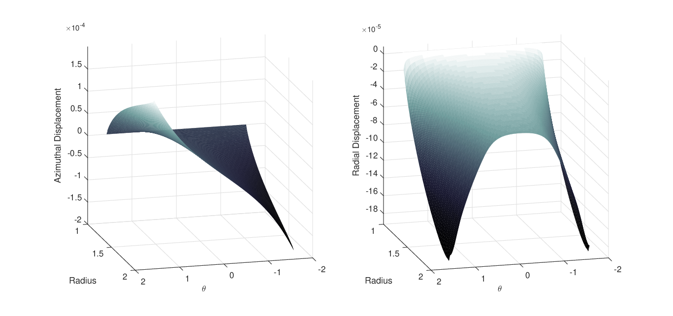
Figure 4: Displacement field of the foundation predicted by the shell on an elastic foundation model with friction, where θ=x2\theta=x^{2}

Fig. 4 is calculated with the values of τmax=1\tau_{\text{max}}=1N/m2\text{m}^{2}, b=2b=2m, h=18h=\frac{1}{8}m, E=8000E=8000Pa, ν=14\nu=\frac{1}{4} and νF=1\nu_{F}=1, and it shows the azimuthal (i.e u2u^{2}) and the radial (i.e. u3u^{3}) displacements. The maximum azimuthal displacements are observed at x2=±12​πx^{2}=\pm\frac{1}{2}\pi, with respective azimuthal displacements of u2=±1.79×10⁻⁴u^{2}=\pm 1.79\times 10^{-4}rad. The maximum radial displacement is observed at x2=±12​πx^{2}=\pm\frac{1}{2}\pi, with a radial displacement of u3=−1.84×10⁻⁴u^{3}=-1.84\times 10^{-4}m. Furthermore, in the intervals x2∈(−1.26,−0.788)x^{2}\in(-1.26,-0.788) and x2∈(0.788,1.26)x^{2}\in(0.788,1.26), we see that the shell is at limiting-equilibrium. These observations simply imply that the shell is more likely to debond from the foundation at the boundaries where we apply external stresses τ0\tau_{0} and τmax\tau_{\text{max}}, and more likely to stay bonded away from the boundary of the shell. Note that all numerical codes are available at http://discovery.ucl.ac.uk/id/eprint/1532145.

3 The Two-Body Coulomb’s Law of Static Friction

The most comprehensive mathematical study on friction that we are aware of is the publication by Kikuchi and Oden [1]. Therefore, in this section, we extend their model to study a two-body friction problem in curvilinear coordinates, and we do so by modifying equation (1) (see section 5.5 (v) of Kikuchi and Oden [1]). Assume that an elastic body on a rough rigid surface where the friction is governed by Coulomb’s law of static friction. Given that one is using curvilinear coordinates, fix the purely-normal stress at the contact boundary as a constant, i.e. νF​T33​(𝒗)|ω+=𝒦\nu_{F}T^{3}_{3}(\boldsymbol{v})|_{\omega^{+}}=\mathscr{K}. Then, equation (1) implies that jε′(𝒗)δ𝒗=−∫ωg3Tα3(𝒗)δvα|ω+dωj_{\varepsilon}^{\prime}(\boldsymbol{v})\delta\boldsymbol{v}=-\int_{\omega}g_{3}T^{3}_{\alpha}(\boldsymbol{v})\delta v^{\alpha}|_{\omega^{+}}~d\omega. Note that 𝒗|ω+\boldsymbol{v}|_{\omega^{+}} describes the relative displacement between the elastic body and the boundary ω\omega, and thus, if the elastic body is in contact with another rough elastic body, then the displacement field one must consider is the relative displacement (due to the fact that friction opposes potential relative motion). Now, consider a two-body contact problem where the contact area is rough and the friction is governed by Coulomb’s law of static friction. Now, let the displacement fields of the overlying body and the foundation be 𝒗\boldsymbol{v} and 𝒖\boldsymbol{u} respectively. As the purely-normal stress is continuous at the boundary, just as before, fix the purely normal stress as νF​T33​(𝒖)|ω−=νF​T33​(𝒗)|ω+=𝒦\nu_{F}T^{3}_{3}(\boldsymbol{u})|_{\omega^{-}}=\nu_{F}T^{3}_{3}(\boldsymbol{v})|_{\omega^{+}}=\mathscr{K}, where ω−=limx3→0−Ω\omega^{-}=\lim_{x^{3}\to 0^{-}}\Omega, and make the transformation vβ|ω+→vβ|ω+−uβ|ω−v^{\beta}|_{\omega^{+}}\to v^{\beta}|_{\omega^{+}}-u^{\beta}|_{\omega^{-}} in the functional jε​(⋅)j_{\varepsilon}(\cdot) to signify the relative displacement field. Now, collecting all the tangential terms from the contact boundary (i.e. uβ|ω−u^{\beta}|_{\omega^{-}} and vβ|ω+v^{\beta}|_{\omega^{+}} terms), one finds jε′(𝒗−𝒖)(δ𝒗−δ𝒖)=−∫ωg3([Tα3(𝒗)δvα]|ω+−[Tα3(𝒖)δuα]|ω−)dωj_{\varepsilon}^{\prime}(\boldsymbol{v}-\boldsymbol{u})(\delta\boldsymbol{v}-\delta\boldsymbol{u})=-\int_{\omega}g_{3}([T^{3}_{\alpha}(\boldsymbol{v})\delta v^{\alpha}]|_{\omega^{+}}-[T^{3}_{\alpha}(\boldsymbol{u})\delta u^{\alpha}]|_{\omega^{-}})~d\omega, where

jε​(𝒗−𝒖)\displaystyle\qquad j_{\varepsilon}(\boldsymbol{v}-\boldsymbol{u}) ={∫ω[𝒦​Φ​(𝒗−𝒖)−12​ε]​𝑑ω,ifΦ(𝒗−𝒖)|ω≥ε,∫ω[12​𝒦​(Φ⁡(𝒗−𝒖))2ε]​𝑑ω,ifΦ(𝒗−𝒖)|ω<ε,\displaystyle=\left\{\begin{aligned} \int_{\omega}\left[\mathscr{K}\Phi(\boldsymbol{v}-\boldsymbol{u})-\frac{1}{2}\varepsilon\right]d\omega&,~\text{if}~\Phi(\boldsymbol{v}-\boldsymbol{u})|_{\omega}\geq\varepsilon,\\ \int_{\omega}\left[\frac{1}{2}\mathscr{K}\frac{\left(\Phi(\boldsymbol{v}-\boldsymbol{u})\right)^{2}}{\varepsilon}\right]d\omega&,~\text{if}~\Phi(\boldsymbol{v}-\boldsymbol{u})|_{\omega}<\varepsilon,\end{aligned}\right.
Φ⁡(𝒗−𝒖)\displaystyle\Phi(\boldsymbol{v}-\boldsymbol{u}) =(ℓα​(𝒗−𝒖)​ℓα​(𝒗−𝒖))12,\displaystyle=\left(\ell_{\alpha}(\boldsymbol{v}-\boldsymbol{u})\ell^{\alpha}(\boldsymbol{v}-\boldsymbol{u})\right)^{\frac{1}{2}},
ℓ⁡(𝒗−𝒖)\displaystyle\boldsymbol{\ell}(\boldsymbol{v}-\boldsymbol{u}) =(v1,v2)|ω+−(u1,u2)|ω−.\displaystyle=\boldsymbol{(}v^{1},v^{2}\boldsymbol{)}|_{\omega^{+}}-\boldsymbol{(}u^{1},u^{2}\boldsymbol{)}|_{\omega^{-}}.

As the two bodies are in contact, the normal displacement (of both bodies) is continuous. Thus, one obtains the modified Kikuchi and Oden’s model for Coulomb’s law of static friction for a two-body problem in curvilinear coordinates, which is described by the following set of equations

v3|ω+−u3|ω−\displaystyle v^{3}|_{\omega^{+}}-u^{3}|_{\omega^{-}} =0,\displaystyle=0,
T33​(𝒗)|ω+−T33​(𝒖)|ω−\displaystyle T_{3}^{3}(\boldsymbol{v})|_{\omega^{+}}-T_{3}^{3}(\boldsymbol{u})|_{\omega^{-}} =0,\displaystyle=0,
T3β(𝒗)|ω+={−νF​g3​(vβ|ω+−uβ|ω−)Φ⁡(𝒗−𝒖)​(T33​(𝒗)|ω+),ifΦ(𝒗−𝒖)|ω+≥ε,−νF​g3​(vβ|ω+−uβ|ω−)ε​(T33​(𝒗)|ω+),ifΦ(𝒗−𝒖)|ω+<ε,\displaystyle\qquad T_{3}^{\beta}(\boldsymbol{v})|_{\omega^{+}}=\left\{\begin{aligned} -\frac{\nu_{F}g_{3}\left(v^{\beta}|_{\omega^{+}}-u^{\beta}|_{\omega^{-}}\right)}{\Phi(\boldsymbol{v}-\boldsymbol{u})}\left(T_{3}^{3}(\boldsymbol{v})|_{\omega^{+}}\right)&,~\text{if}~\Phi(\boldsymbol{v}-\boldsymbol{u})|_{\omega^{+}}\geq\varepsilon,\\ -\frac{\nu_{F}g_{3}\left(v^{\beta}|_{\omega^{+}}-u^{\beta}|_{\omega^{-}}\right)}{\varepsilon}\left(T_{3}^{3}(\boldsymbol{v})|_{\omega^{+}}\right)&,~\text{if}~\Phi(\boldsymbol{v}-\boldsymbol{u})|_{\omega^{+}}<\varepsilon,\end{aligned}\right.
T3β(𝒖)|ω−={−νF​g3​(vβ|ω+−uβ|ω−)Φ⁡(𝒗−𝒖)​(T33​(𝒖)|ω−),ifΦ(𝒗−𝒖)|ω−≥ε,−νF​g3​(vβ|ω+−uβ|ω−)ε​(T33​(𝒖)|ω−),ifΦ(𝒗−𝒖)|ω−<ε,\displaystyle\qquad T_{3}^{\beta}(\boldsymbol{u})|_{\omega^{-}}=\left\{\begin{aligned} -\frac{\nu_{F}g_{3}\left(v^{\beta}|_{\omega^{+}}-u^{\beta}|_{\omega^{-}}\right)}{\Phi(\boldsymbol{v}-\boldsymbol{u})}\left(T_{3}^{3}(\boldsymbol{u})|_{\omega^{-}}\right)&,~\text{if}~\Phi(\boldsymbol{v}-\boldsymbol{u})|_{\omega^{-}}\geq\varepsilon,\\ -\frac{\nu_{F}g_{3}\left(v^{\beta}|_{\omega^{+}}-u^{\beta}|_{\omega^{-}}\right)}{\varepsilon}\left(T_{3}^{3}(\boldsymbol{u})|_{\omega^{-}}\right)&,~\text{if}~\Phi(\boldsymbol{v}-\boldsymbol{u})|_{\omega^{-}}<\varepsilon,\end{aligned}\right.

where

T3β​(𝒗)\displaystyle T^{\beta}_{3}(\boldsymbol{v}) =μ⁡(∇¯β​v3+∇¯3​vβ),\displaystyle=\mu\left(\bar{\nabla}^{\beta}v_{3}+\bar{\nabla}_{\!3}v^{\beta}\right),
T33​(𝒗)\displaystyle T^{3}_{3}(\boldsymbol{v}) =λ​∇¯α​vα+(λ+2​μ)​∇¯3​v3,\displaystyle=\lambda\bar{\nabla}_{\!\alpha}v^{\alpha}+\left(\lambda+2\mu\right)\bar{\nabla}_{\!3}v^{3},
T3β​(𝒖)\displaystyle T^{\beta}_{3}(\boldsymbol{u}) =μ¯​(∇¯β​u3+∇¯3​uβ),\displaystyle=\bar{\mu}\left(\bar{\nabla}^{\beta}u_{3}+\bar{\nabla}_{\!3}u^{\beta}\right),
T33​(𝒖)\displaystyle T^{3}_{3}(\boldsymbol{u}) =λ¯​∇¯α​uα+(λ¯+2​μ¯)​∇¯3​u3,\displaystyle=\bar{\lambda}\bar{\nabla}_{\!\alpha}u^{\alpha}+\left(\bar{\lambda}+2\bar{\mu}\right)\bar{\nabla}_{\!3}u^{3},

and where νF\nu_{F} is the coefficient of friction. Note that given that T33​(𝒖)|ω−T^{3}_{3}(\boldsymbol{u})|_{\omega^{-}} is fixed as a positive constant and considering Euclidean coordinates, then the above problem simply reduces to the Kikuchi and Oden’s original model for Coulomb’s law of static friction [1] in the limit 𝒖→0\boldsymbol{u}\to 0. Also, the above modified Kikuchi and Oden’s model can further be simplified by noticing that the continuousness of the purely-normal stress at the boundary; however, from our numerical analysis, we find that this reduced model is non-convergent in a finite-difference setting. Thus, we insist upon the given formulation.

3.1 A Numerical Example

To proceed with our analysis, we numerically model the overlying body as a three-dimensional body and we do not approximate this body as a shell or otherwise. Thus, the displacement at the contact region with this approach is obtained by the use of the standard equilibrium equations in linear elasticity and the modified Kikuchi and Oden’s model.

In accordance with the framework that is introduced in section 2.2, the overlying body is restricted to the region x3∈(0,h)x^{3}\in(0,h). Now, we can express the governing equations of the overlying body as follows

(λ+μ)​∂2(∇¯i​vi)+μ​(ψ¯2)2​Δ¯​v2\displaystyle(\lambda+\mu)\partial_{2}(\bar{\nabla}_{\!i}v^{i})+\mu(\bar{\psi}_{2})^{2}\bar{\Delta}v^{2} =0,\displaystyle=0,
(λ+μ)​∂3(∇¯i​vi)+μ​Δ¯​v3\displaystyle(\lambda+\mu)\partial_{3}(\bar{\nabla}_{\!i}v^{i})+\mu\bar{\Delta}v^{3} =0,\displaystyle=0,

where 𝒗=(0,v2​(x2,x3),v3​(x2,x3))\boldsymbol{v}=\boldsymbol{(}0,v^{2}(x^{2},x^{3}),v^{3}(x^{2},x^{3})\boldsymbol{)} is the displacement field of the overlying body, the perturbed governing equations of the overlying body as follows

(λ+μ)​∂2(∇¯i​δ​vi)+μ​(ψ¯2)2​Δ¯​δ​v2\displaystyle(\lambda+\mu)\partial_{2}(\bar{\nabla}_{\!i}\delta v^{i})+\mu(\bar{\psi}_{2})^{2}\bar{\Delta}\delta v^{2} =0,\displaystyle=0,
(λ+μ)​∂3(∇¯i​δ​vi)+μ​Δ¯​δ​v3\displaystyle(\lambda+\mu)\partial_{3}(\bar{\nabla}_{\!i}\delta v^{i})+\mu\bar{\Delta}\delta v^{3} =0,\displaystyle=0,

where δ​𝒗=(0,δ​v2​(x2,x3),δ​v3​(x2,x3))\delta\boldsymbol{v}=\boldsymbol{(}0,\delta v^{2}(x^{2},x^{3}),\delta v^{3}(x^{2},x^{3})\boldsymbol{)} is a small perturbation of the displacement field of the overlying body, and the perturbed governing equations of the foundation as follows

(λ¯+μ¯)​∂2(∇¯i​δ​ui)+μ¯​(ψ¯2)2​Δ¯​δ​u2\displaystyle(\bar{\lambda}+\bar{\mu})\partial_{2}(\bar{\nabla}_{\!i}\delta u^{i})+\bar{\mu}(\bar{\psi}_{2})^{2}\bar{\Delta}\delta u^{2} =0,\displaystyle=0,
(λ¯+μ¯)​∂3(∇¯i​δ​ui)+μ¯​Δ¯​δ​u3\displaystyle(\bar{\lambda}+\bar{\mu})\partial_{3}(\bar{\nabla}_{\!i}\delta u^{i})+\bar{\mu}\bar{\Delta}\delta u^{3} =0,\displaystyle=0,

where δ​𝒖=(0,δ​u2​(x2,x3),δ​u3​(x2,x3))\delta\boldsymbol{u}=\boldsymbol{(}0,\delta u^{2}(x^{2},x^{3}),\delta u^{3}(x^{2},x^{3})\boldsymbol{)} is the perturbation of the displacement field of the foundation. Also, we can express the boundary conditions of the overlying body as follows

[(λ+2​μ)​∂2v2+λ⁡(∂3v3+Γ¯222​v2+Γ¯232​v3)]|{∂ωT0New,∂ωTmaxNew}×[0,h]\displaystyle\big[(\lambda+2\mu)\partial_{2}v^{2}+\lambda\left(\partial_{3}v^{3}+\bar{\Gamma}^{2}_{\!22}v^{2}+\bar{\Gamma}^{2}_{\!23}v^{3}\right)\big]|_{\{\partial\omega_{T_{0}}^{\text{New}},\partial\omega_{T_{\text{max}}}^{\text{New}}\}\times[0,h]} ={τ0,τmax},\displaystyle=\{\tau_{0},\tau_{\text{max}}\},
[λ⁡(∂2v2+Γ¯222​v2+Γ¯232​v3)+(λ+2​μ)​∂3v3]|(−12​π,12​π)×{h}\displaystyle\big[\lambda\left(\partial_{2}v^{2}+\bar{\Gamma}^{2}_{\!22}v^{2}+\bar{\Gamma}^{2}_{\!23}v^{3}\right)+(\lambda+2\mu)\partial_{3}v^{3}\big]|_{(-\frac{1}{2}\pi,\frac{1}{2}\pi)\times\{h\}} =0,\displaystyle=0,
[(ψ¯2)2​∂3v2+∂2v3]|{∂ωNew×[0,h]}∪{(−12​π,12​π)×{h}}\displaystyle\big[(\bar{\psi}_{2})^{2}\partial_{3}v^{2}+\partial_{2}v^{3}\big]|_{\{\partial\omega^{\text{New}}\times[0,h]\}\cup\{(-\frac{1}{2}\pi,\frac{1}{2}\pi)\times\{h\}\}} =0,\displaystyle=0,

boundary conditions of the displacement fields as follows

[v3−u3]|ωNew\displaystyle\big[v^{3}-u^{3}\big]|_{\omega^{\text{New}}} =0​(continuous radial displacement),\displaystyle=0~\text{(continuous radial displacement)},
[T33​(𝒗)−T33​(𝒖)]|ωNew\displaystyle\big[T^{3}_{3}(\boldsymbol{v})-T^{3}_{3}(\boldsymbol{u})\big]|_{\omega^{\text{New}}} =0​(continuous radial stress),\displaystyle=0~\text{(continuous radial stress)},

and the boundary conditions of the perturbations as follows,

δ​u2|∂Ω0New∪∂Ω¯fNew\displaystyle\delta u^{2}|_{\partial\Omega_{0}^{\text{New}}\cup\overline{\partial\Omega}_{f}^{\text{New}}} =0,\displaystyle=0,
δ​u3|∂Ω¯New\displaystyle\delta u^{3}|_{\overline{\partial\Omega}^{\text{New}}} =0,\displaystyle=0,
δ​v2|{∂ωNew×(0,h)}∪{[−12​π,12​π]×{h}}\displaystyle\delta v^{2}|_{\{\partial\omega^{\text{New}}\times(0,h)\}\cup\{[-\frac{1}{2}\pi,\frac{1}{2}\pi]\times\{h\}\}} =0,\displaystyle=0,
δ​v3|ω¯New∪{∂ωNew×(0,h)}∪{[−12​π,12​π]×{h}}\displaystyle\delta v^{3}|_{\bar{\omega}^{\text{New}}\cup\{\partial\omega^{\text{New}}\times(0,h)\}\cup\{[-\frac{1}{2}\pi,\frac{1}{2}\pi]\times\{h\}\}} =0.\displaystyle=0.

Thus, the equations characterising the frictional coupling of the overlying body to the foundation can be expressed as follows:
If ψ2​|v2−u2||ωNew≥ϵ\psi_{2}|v^{2}-u^{2}||_{\omega^{\text{New}}}\geq\epsilon, then

[μ⁡(ψ2​∂3v2+(ψ2)−1​∂2v3)+νF​sign​(v2−u2)​T33​(𝒗)]|ωNew\displaystyle\big[\mu\left(\psi_{2}\partial_{3}v^{2}+(\psi_{2})^{-1}\partial_{2}v^{3}\right)+\nu_{F}\mathrm{sign}(v^{2}-u^{2})T^{3}_{3}(\boldsymbol{v})\big]|_{\omega^{\text{New}}} =0,\displaystyle=0,
[μ¯​(ψ2​∂3u2+(ψ2)−1​∂2u3)+νF​sign​(v2−u2)​T33​(𝒖)]|ωNew\displaystyle\big[\bar{\mu}\left(\psi_{2}\partial_{3}u^{2}+(\psi_{2})^{-1}\partial_{2}u^{3}\right)+\nu_{F}\mathrm{sign}(v^{2}-u^{2})T^{3}_{3}(\boldsymbol{u})\big]|_{\omega^{\text{New}}} =0;\displaystyle=0;

If ψ2​|v2−u2||ωNew<ϵ\psi_{2}|v^{2}-u^{2}||_{\omega^{\text{New}}}<\epsilon, then

[μ(ψ2∂3δv2)+νFϵ−1ψ2(v2−u2)T33(δ𝒗)+νFϵ−1ψ2(δv2−δu2)T33(𝒗)\displaystyle\big[\mu\left(\psi_{2}\partial_{3}\delta v^{2}\right)+\nu_{F}\epsilon^{-1}\psi_{2}(v^{2}-u^{2})T^{3}_{3}(\delta\boldsymbol{v})+\nu_{F}\epsilon^{-1}\psi_{2}(\delta v^{2}-\delta u^{2})T^{3}_{3}(\boldsymbol{v})
+μ⁡(ψ2​∂3v2+(ψ2)−1​∂2v3)+νF​ϵ−1​ψ2​(v2−u2)​T33​(𝒗)\displaystyle+\mu\left(\psi_{2}\partial_{3}v^{2}+(\psi_{2})^{-1}\partial_{2}v^{3}\right)+\nu_{F}\epsilon^{-1}\psi_{2}(v^{2}-u^{2})T^{3}_{3}(\boldsymbol{v}) ]|ωNew=0,\displaystyle\big]|_{\omega^{\text{New}}}=0,
[μ¯(ψ2∂3δu2)+νFϵ−1ψ2(v2−u2)T33(δ𝒖)+νFϵ−1ψ2(δv2−δu2)T33(𝒖)\displaystyle\big[\bar{\mu}\left(\psi_{2}\partial_{3}\delta u^{2}\right)+\nu_{F}\epsilon^{-1}\psi_{2}(v^{2}-u^{2})T^{3}_{3}(\delta\boldsymbol{u})+\nu_{F}\epsilon^{-1}\psi_{2}(\delta v^{2}-\delta u^{2})T^{3}_{3}(\boldsymbol{u})
+μ¯​(ψ2​∂3u2+(ψ2)−1​∂2u3)+νF​ϵ−1​ψ2​(v2−u2)​T33​(𝒖)\displaystyle+\bar{\mu}\left(\psi_{2}\partial_{3}u^{2}+(\psi_{2})^{-1}\partial_{2}u^{3}\right)+\nu_{F}\epsilon^{-1}\psi_{2}(v^{2}-u^{2})T^{3}_{3}(\boldsymbol{u}) ]|ωNew=0,\displaystyle\big]|_{\omega^{\text{New}}}=0,

where

T33​(𝒗)\displaystyle T^{3}_{3}(\boldsymbol{v}) =λ⁡(∂2v2+Γ¯222​v2+Γ¯232​v3)+(λ+2​μ)​∂3v3,\displaystyle=\lambda\left(\partial_{2}v^{2}+\bar{\Gamma}^{2}_{\!22}v^{2}+\bar{\Gamma}^{2}_{\!23}v^{3}\right)+(\lambda+2\mu)\partial_{3}v^{3},
T33​(𝒖)\displaystyle T^{3}_{3}(\boldsymbol{u}) =λ¯​(∂2u2+Γ¯222​u2+Γ¯232​u3)+(λ¯+2​μ¯)​∂3u3.\displaystyle=\bar{\lambda}\left(\partial_{2}u^{2}+\bar{\Gamma}^{2}_{\!22}u^{2}+\bar{\Gamma}^{2}_{\!23}u^{3}\right)+(\bar{\lambda}+2\bar{\mu})\partial_{3}u^{3}.

To conduct numerical experiments, we use the second-order accurate iterative-Jacobi finite-difference method with Newton’s method for nonlinear systems (see chapter 10 of Burden et al. [29]). Also, as a result of the grid dependence in the overlying body, we must satisfy the condition ψ0​Δ​x2≤Δ​x3\psi_{0}\Delta x^{2}\leq\Delta x^{3}, ∀ψ0∈{ψ¯2​(x2,x3)∣x2∈[−12​π,12​π]​and​x3∈[0,h]}\forall~\psi_{0}\in\{\bar{\psi}_{2}(x^{2},x^{3})\mid x^{2}\in[-\frac{1}{2}\pi,\frac{1}{2}\pi]~\text{and}~x^{3}\in[0,h]\}. For our purposes, we let Δ​x2=1N−1​π\Delta x^{2}=\frac{1}{N-1}\pi and ψ0=ψ¯2​(14​π,h)\psi_{0}=\bar{\psi}_{2}(\frac{1}{4}\pi,h), where N=250N=250.

Refer to caption
Figure 5: Displacement field of the foundation of the modified Kikuchi and Oden’s model, where θ=x2\theta=x^{2}

Fig. 5 is calculated with the values τmax=1\tau_{\text{max}}=1N/m2\text{m}^{2}, b=2b=2m, h=18h=\frac{1}{8}m, E=8000E=8000Pa, ν=14\nu=\frac{1}{4}, ε=10−10\varepsilon=10^{-10}m, and νF=1\nu_{F}=1, and it shows the azimuthal (i.e. u2u^{2}) and the radial (i.e. u3u^{3}) displacements of the foundation. The maximum azimuthal displacements are observed at x2=±12​πx^{2}=\pm\frac{1}{2}\pi with respective azimuthal displacements of u2=±1.70×10⁻⁴u^{2}=\pm 1.70\times 10^{-4}rad. The maximum radial displacement is observed at x2=±12​πx^{2}=\pm\frac{1}{2}\pi with a radial displacement of u3=−1.85×10⁻⁴u^{3}=-1.85\times 10^{-4}m. Also, in the interval x2∈(−12​π,12​π)x^{2}\in(-\frac{1}{2}\pi,\frac{1}{2}\pi), i.e. in the entire contact region, we see that the overlying body is at limiting-equilibrium. Just as it is in the analysis of Fig. 4, these observations simply imply that the shell is more likely to debond from foundation at the boundaries where we apply external stress, and more likely to stay bonded away from those boundaries. However, Fig. 5 predicts a higher likelihood of debonding relative to the shell model as now the entire contact region is at limiting-equilibrium for the two-body Coulomb’s law of static friction.

3.2 Comparing a Shell Frictionally Coupled to an Elastic Foundation and Two-Body Coulomb’s Law of Static Friction

Our final goal in this section is to investigate how our model for a shell on an elastic foundation with friction predicts the displacement field of the foundation relative to the two-body elastic model with friction. From this, we should be able to ascertain how the stresses from the thin body (approximated by a shell or otherwise) propagate to the foundation and deforms it, and we do this for the variables νF\nu_{F}, δ​τ=τmax/τ0\delta\tau=\tau_{\text{max}}/\tau_{0}, δ​b=b/a\delta b=b/a, δ​h=h/L\delta h=h/L, δ​E=E/E¯\delta E=E/\bar{E} and δ​ν=ν/ν¯\delta\nu=\nu/\bar{\nu}. To calculate the relative error between the displacement field of the foundation predicted by each model, we define the following metric

RelativeError⁡(ui)=∑{k,l}‖ushell-modeli​(yk2,yl3)−uKikuchi-Odeni​(yk2,yl3)‖2∑{k,l}‖ushell-modeli​(yk2,yl3)‖2+‖uKikuchi-Odeni​(yk2,yl3)‖2,\displaystyle\mathrm{RelativeError}(u^{i})=\frac{\sqrt{\sum_{\{k,l\}}||u_{\text{shell-model}}^{i}(y^{2}_{k},y^{3}_{l})-u_{\text{Kikuchi-Oden}}^{i}(y^{2}_{k},y^{3}_{l})||^{2}}}{\sqrt{\sum_{\{k,l\}}||u_{\text{shell-model}}^{i}(y^{2}_{k},y^{3}_{l})||^{2}+||u_{\text{Kikuchi-Oden}}^{i}(y^{2}_{k},y^{3}_{l})||^{2}}},

where yk2=−12​π+k​Δ​x2y^{2}_{k}=-\frac{1}{2}\pi+k\Delta x^{2}, yl3=−L+l​Δ​x3y^{3}_{l}=-L+l\Delta x^{3}, 0≤k≤(N−1)0\leq k\leq(N-1) and 0≤l≤(N−1)0\leq l\leq(N-1). Note that we assume the default values νF=1\nu_{F}=1, δ​τ=1\delta\tau=1, δ​b=1\delta b=1, δ​h=18\delta h=\frac{1}{8}, δ​E=8\delta E=8 and δ​ν=1\delta\nu=1 and ε=10−10\varepsilon=10^{-10}m throughout, unless it strictly says otherwise.

Refer to caption
Figure 6: Relative error for νF\nu_{F}
Refer to caption
Figure 7: Relative error for δ​τ\delta\tau
Refer to caption
Figure 8: Relative error for δ​h\delta h
Refer to caption
Figure 9: Relative error for δ​E\delta E
Refer to caption
Figure 10: Relative error for δ​ν\delta\nu
Refer to caption
Figure 11: Relative error for δ​b\delta b

Fig. 6 shows that as the coefficient of friction at the contact region, νF\nu_{F}, increases, the relative errors decrease, and this reduction in the error is significant in its magnitude. This implies that rougher the contact surface is, then closer our shell model with friction resembles the modified Kikuchi and Oden’s model. This is an intuitive result as the coefficient of friction increases, both models resemble the bonded case, and in chapter 3 of Jayawardana [3], it is shown that the our bonded shell model is a better approximation of the overlying body with respect to the asymptotic model implied by Baldelli and Bourdin’s method [30].

Fig. 7 shows that as the traction ratio, δ​τ\delta\tau, increases, both azimuthal and radial relative errors also increase. This implies that the limiting-equilibriums implied by each model can be very different. We observed this effect in our earlier numerical modelling (recall the analysis of Fig. 4 and Fig. 5).

Fig. 8 shows that as the relative thickness of the shell, δ​h\delta h, decreases, both the azimuthal and the radial relative errors increase. This is contradicts the derivation assumptions of our shell model with friction as we derived our displacement-based friction condition by considering Coulomb’s law to remain valid in the limit δ​h→0\delta h\to 0, and thus, we should expect a better agreement between the two models for smaller values of δ​h\delta h.

Fig. 9 shows the that as the relative Young’s modulus of the shell, δ​E\delta E, increases, the relative errors decrease. If one assumes the shell is bonded to the elastic foundation, then this result seems to be consistent with Aghalovyan’s asymptotic analysis of the modulus of an orthotropic foundation and two-layer anisotropic plates [31].

Fig. 10 shows that as the relative Poisson’s ratio of the shell, δ​ν\delta\nu, increases, the relative error decreases. This implies that as the shell becomes incompressible, both models would be in better agreement.

Fig. 11 shows that as δ​b\delta b decreases, both azimuthal and radial relative errors also decrease. Assuming the contact region x2∈(−12​π,12​π)x^{2}\in(-\frac{1}{2}\pi,\frac{1}{2}\pi) (with OPENx2≠±12​π)x^{2}\neq\pm\frac{1}{2}\pi), this result may be interpreted as follows: as the radius of curvature of the contact region increases, the relative errors decrease. Note that we derived our shell equation to be valid for contact regions with high radius of curvatures (see condition 1).

Remark 1.

In a different study, to ascertain the physical validity of our shell model with friction, we conduct human trials to measure the frictional interactions that fabrics have on soft-tissue of human subjects: 10 subjects in the first trial and 8 subjects in the second trial (see chapter 6 of Jayawardana [3]). We discover the following: (i) a positive correlation between the displacement of soft-tissue and the volume of soft-tissue; (ii) a positive correlation between the applied tension to the fabric and the volume of soft-tissue; (iii) a negative correlation between the displacement of the soft-tissue and the Young’s modulus of soft-tissue; and (iv) a negative correlation between the applied tension to the fabric and the Young’s modulus of soft-tissue. From further numerical modellings of our shell model with friction (where now the shell is approximated with a shell-membrane) we were able to predict the correlations-(i) to (iii). However, our numerical modelling could not predict correlation-(iv). It is unclear whether the discrepancy in correlation-(iv) is due to a flaw in our numerical modelling (see section 3 of Jayawardana et al. [6]) or our data analysis of the experiments.

4 Conclusions

In our analysis, we derived a model for a shell that is frictionally coupled to an elastic foundation. We used Kikuchi and Oden’s model for Coulomb’s law of static friction [1] to derive a displacement-based static-friction condition. By construction, this displacement-based friction condition is mathematically sound as we proved the existence and the uniqueness of solutions for our shell model with friction with the aid of the work of Kinderlehrer and Stampacchia [2] (and section 8.4.2 of Evans [25]). Note that, as far as we are aware, this is the first derivation of a displacement-based friction condition, as only force, stress and energy based friction conditions currently exist in the literature.

For numerical analysis, we modified Kikuchi and Oden’s model for Coulomb’s law of static friction [1] to model a full two-body elasticity contact problem in curvilinear coordinates. The purpose of numerical analysis is to ascertain how the displacement field of the foundation behaves when the overlying body is modelled with our shell model with friction in comparison to when the overlying body is modelled with standard equilibrium equations in linear elasticity and modified Kikuchi and Oden’s model. Note that, as far as we are aware, this is the first derivation of a two-body 3D (and 2D) elasticity contact problem with friction, as only one-body elasticity contact problems (one elastic-body in contact with one rigid-body) and two-body 1D elasticity contact problems (see analysis of elastic strings in contact [19, 20, 21, 22]) with friction, currently exist in the literature. The numerical results indicate that, if the shell has a relatively high Young’s modulus (i.e. stiff) or has a relatively high Poisson’s ratio (i.e. close to incompressible), and the contact region has a high coefficient of friction or has a high radius of curvature, then the displacement field of the foundation predicted by both models are in better agreement. We also observed that both models are in better agreement for thicker shells, which is a contradictory result as it is inconsistent with the derivation of our shell model with friction; therefore, further research is needed to resolve this contradiction.

From our numerical analysis, the greatest reduction in the error is observed for higher coefficients of friction, i.e. as the coefficient of friction increases, the bodies behaves as if they are bonded, and thus, the greater agreement between the solutions of both models. This is an expected result as our overlying shell model was initially derived to approximate bonded thin bodies on elastic foundations, and the efficacy of this model is numerically demonstrated in sections 3.5 and 3.6 of Jayawardana [3]. The second greatest reduction in the error is observed for higher Young’s moduli of the shell. This is also an expected result as it seems to be consistent with the asymptotic analysis of similar problems (given that the shell is bonded to the elastic foundation) by Aghalovyan [31].

On a final note, given that the thin body is further approximated by a shell-membrane (i.e. neglecting bending effects of the shell), our model can be use to investigate the frictional interactions between fabrics and human soft-tissue (i.e. the stresses on human skin and the deformation of the subcutaneous tissue due to friction generated by everyday attire). A detail study of this can be found in chapter 6 of Jayawardana [3] and Jayawardana et al. [6].

Acknowledgments

We thank Dr Nick Ovenden (UCL) and Prof Alan Cottenden (UCL) for their supervision, Brad Turner (TEKOR) for his assistance, and Christopher Law for the illustrations.

References

  • [1] N. Kikuchi, J. T. Oden, Contact problems in elasticity: a study of variational inequalities and finite element methods, SIAM, 1988.
  • [2] D. Kinderlehrer, G. Stampacchia, An introduction to variational inequalities and their applications, SIAM, 2000.
  • [3] K. Jayawardana, Mathematical theory of shells on elastic foundations: an analysis of boundary forms, constraints, and applications to friction and skin abrasion, Ph.D. thesis, UCL (University College London) (2016).
  • [4] F. P. Bowden, F. P. Bowden, D. Tabor, The friction and lubrication of solids, Vol. 1, Oxford university press, 2001.
  • [5] S. K. Clark, Mechanics of pneumatic tires, US Government Printing Office, 1981.
  • [6] K. Jayawardana, N. C. Ovenden, A. Cottenden, Quantifying the frictional forces between skin and nonwoven fabrics, Frontiers in physiology 8 (2017) 107.
  • [7] W. F. Bergfeld, J. S. Taylor, Trauma, sports, and the skin, American journal of industrial medicine 8 (4-5) (1985) 403–413.
  • [8] J. Asserin, H. Zahouani, P. Humbert, V. Couturaud, D. Mougin, Measurement of the friction coefficient of the human skin in vivo: quantification of the cutaneous smoothness, Colloids and surfaces B: Biointerfaces 19 (1) (2000) 1–12.
  • [9] F. Levit, Jogger’s nipples., The New England journal of medicine 297 (20) (1977) 1127–1127.
  • [10] D. S. Wilkinson, Dermatitis from repeated trauma to the skin, American journal of industrial medicine 8 (4-5) (1985) 307–317.
  • [11] J. Maklebust, M. Sieggreen, Pressure ulcers: Guidelines for prevention and management, Lippincott Williams & Wilkins, 2001.
  • [12] A. B. Shrank, The aetiology of juvenile plantar dermatosis, British Journal of Dermatology 100 (6) (1979) 641–648.
  • [13] K. L. Johnson, Contact mechanics, Cambridge university press, 1987.
  • [14] D. Quadling, H. Neill, Mechanics 1, Cambridge Advanced Level Mathematics for OCR, Cambridge University Press, 2004.
  • [15] M. Badiale, E. Serra, Semilinear Elliptic Equations for Beginners: Existence Results via the Variational Approach, Springer Science & Business Media, 2010.
  • [16] P. G. Ciarlet, An introduction to differential geometry with applications to elasticity, Journal of Elasticity 78 (1) (2005) 1–215.
  • [17] C. L. RAO, J. Lakshinarashiman, R. Sethuraman, S. M. Sivakumar, Engineering Mechanics: Statics and Dynamics, PHI Learning Pvt. Ltd., 2003.
  • [18] D. Y. Gao, Finite deformation beam models and triality theory in dynamical post-buckling analysis, International journal of non-linear mechanics 35 (1) (2000) 103–131.
  • [19] S. Döonmez, A. Marmarali, A model for predicting a yarn’s knittability, Textile research journal 74 (12) (2004) 1049–1054.
  • [20] P. Grandgeorge, C. Baek, H. Singh, P. Johanns, T. G. Sano, A. Flynn, J. H. Maddocks, P. M. Reis, Mechanics of two filaments in tight orthogonal contact, Proceedings of the National Academy of Sciences 118 (15) (2021).
  • [21] J. H. Maddocks, J. B. Keller, Ropes in equilibrium, SIAM Journal on Applied Mathematics 47 (6) (1987) 1185–1200.
  • [22] P. B. Warren, R. C. Ball, R. E. Goldstein, Why clothes don’t fall apart: Tension transmission in staple yarns, Physical review letters 120 (15) (2018) 158001.
  • [23] R. A. Adams, J. J. Fournier, Sobolev spaces, Elsevier, 2003.
  • [24] D. C. Kay, Schaum’s Outline of Tensor Calculus, McGraw Hill Professional, 1988.
  • [25] L. C. Evans, Partial differential equations, Graduate studies in mathematics 19 (4) (1998) 7.
  • [26] R. L. Schilling, Measures, integrals and martingales, Cambridge University Press, 2017.
  • [27] J. N. Reddy, Theory and analysis of elastic plates and shells, CRC press, 2006.
  • [28] P. Moon, D. E. Spencer, Field theory handbook: including coordinate systems, differential equations and their solutions, Springer, 2012.
  • [29] R. Burden, J. Faires, A. Burden, Numerical Analysis, Cengage Learning, 2015.
  • [30] A. A. L. Baldelli, B. Bourdin, On the asymptotic derivation of winkler-type energies from 3d elasticity, Journal of Elasticity 121 (2) (2015) 275–301.
  • [31] L. A. Aghalovyan, Asymptotic theory of anisotropic plates and shells, World Scientific, 2015.