On Radiation-Based Thermal Servoing:
New Models, Controls and Experiments

Although thermal sensing is a mature technology and has a rich history in the automation of many tasks (see e.g. [7, 8, 9, 10]), its use as a feedback signal for robot control has not been sufficiently studied in the literature [11], where only a few works have addressed this challenging servo-control problem. Some representative works that deal with explicit thermal control include: [12], where a fuzzy controller is developed to regulate the temperature of a fuel cell actuator; [13], where the influence of temperature in the deformation behavior of a surgical robot is investigated, and an explicit thermal regulator is designed; [14], where a control method is designed to maintain a constant tool temperature by adjusting the spindle speed in a stir friction welding robot. However, in these types of methods, temperature control is achieved by directly modulating the power of the heat-generating components. This approach is not suitable when considering external heat sources, e.g. wildfires [15] and sunlight [16], or when the source’s power should not be varied, e.g. in cosmetic procedures [17].

A different strategy is to use sensor-based control, i.e. to dynamically change the source-object geometric configuration to achieve a desired thermal response (similar to what many organisms do [18]). This can be easily done by rigid robots, since their basic function is motion control. Such approach demands the development of appropriate models that can effectively capture the system’s GTM relations. This idea has been partially demonstrated in [19], where the optimal fixed location of multiple radiating heaters in a process is automatically calculated to evenly imprint a desired thermal profile onto a surface. Yet, the heater is static and the method requires exact knowledge of all thermodynamic parameters (which are generally unknown). The proposed approach has also the potential to be used e.g. in fire-fighting [20] or volcano exploration robots [21] to calculate optimal trajectories that avoid overheating or damaging the robot’s components.

The dynamic coupling between temperature and motion may seem unintuitive for humans [22]. Yet, many organisms extensively exploit these relations. For instance, marine animals that inhabit hydro-thermal vents manage their energetic demands by controlling their proximity to the source [23]. Butterflies increase their body temperature by basking dorsally/laterally to maximize sun expose [24]. Ground-dwelling insects adaptively change their body configuration with respect to the sun-heated ground to regulate their temperature [25]. Such advanced thermoception-based behaviors can be used to solve many real-world problems (see Fig. 1). However, these capabilities have not yet been fully incorporated in robot control, a discipline with good track record of borrowing inspiration from nature [26, 27, 28], but which seems to be lagging in this direction.

As a feasible solution to the above-mentioned issues, in this paper, we present a rigorous formulation for robot thermal servoing with radiative sources. The main contributions are summarized as follows:

• •

  We develop an efficient algorithm for computing in real-time the radiation-based thermal interaction matrix which relates robot velocity and object temperature rate.

• •

  We present a novel robot control method for automatically regulating the temperature of grasped objects.

• •

  We report a detailed experimental study to validate the proposed theory.

To the best of the authors’ knowledge, this is the first time that temperature regulation has been formulated in the literature as a robot servoing problem. The proposed approach has the potential to advance the development of multimodal motion controllers for robots.

The rest of the paper is as follows: Section II presents the mathematical models; Section III derives the controller; Section IV reports results; Section V gives final conclusions.

Throughout this manuscript, we denote all column vectors by small bold letters, e.g. $\mathbf{v}\in\mathbb{R}^{n\times 1}$, and matrices by capital bold letters, e.g. $\mathbf{M}\in\mathbb{R}^{m\times n}$.

In the following sections, we introduce basic thermodynamic concepts (we refer the reader to [29, 30]) that are needed for developing the system’s GTM model. To this end, consider a robot manipulator with end-effector configuration denoted by a vector $\mathbf{x}\in\mathbb{R}^{n}$. The robot rigidly grasps (through an adiabatic layer) a planar object whose surface temperature is to be controlled by changing the relative pose to a heat source. The heat transfer model is composed of three main parts (depicted in Fig. 2): (i) heat source, (ii) heat collector (i.e. the object), and (iii) surrounding environment. Thermophysical parameters of different parts are denoted by the same symbol but with different subscripts. We denote the (constant) temperature of the heat source and the (varying) temperature of the object by ${T}_{1}$ and $T_{2}$, respectively. We assume both temperatures to be spatially uniform during the heat transfer process. The environment temperature (assumed to be constant) is denoted by ${T}_{3}$.

Heat transfer occurs amongst the three parts whenever ${T}_{1}$, ${T}_{2},{T}_{3}$ have different values. The direction of heat transfer is always from a high temperature part to a low temperature part. We denote the net energy transfer rate to the object by $Q_{2}$, where a positive value indicates energy inflow. We introduce $q_{2}=Q_{2}/A_{2}$ to represent the surface’s net heat flux and $v=\mathop{}\!\mathrm{d}T_{2}/\mathop{}\!\mathrm{d}t$ to describe the temporal change of the measured temperature ${T}_{2}$. According to the energy conservation laws, these quantities satisfy the relation:

where $m_{2}$ denotes object’s mass and $c_{2}$ denotes the material’s specific heat. To synthesize a thermal servoing controller, it is useful to find an expression of the following form:

which describes the thermal-geometric relation between the robot configuration and the temperature rate.

In this subsection, we show how to calculate $Q_{2}$ between planar surfaces when thermophysical properties are known. According to different mechanisms involved in the heat transfer processes [31], the object’s net heat flux $q_{2}$ satisfies the expression $q_{2}=q_{rad}+q_{conv}+{q}_{cond}$, for radiative ${q}_{rad}$, convective ${q}_{conv}$ and conductive ${q}_{cond}$ fluxes. In our case of study, thermal radiation is the dominant heat transfer mode; Note that $q_{cond}$ and $q_{conv}$ are negligible since the object is grasped through an adiabatic layer and the source’s temperature is much higher than those of the object and environment.

The net energy transfer rate ${Q_{2}}$ has the following form:

where $A_{2}$ denotes the object’s surface area, $G_{2}$ the radiative flux incident at the surface, $\alpha_{2}\in[0,1]$ the object’s absorptance and $E_{2}$ the heat flux emitted by a surface (i.e. emissive power) which is approximated using the Stefan-Boltsman law [29]

with $\varepsilon_{2}\in[0,1]$ the material’s emittance, and $\sigma$ is the Stefan-Boltzmann constant.

Note that for an opaque surface (i.e. with zero transmittance), its reflectance $\rho_{i}$ and absorptance $\alpha_{i}$ satisfy $\rho_{i}+{\alpha}_{i}=1$. Radiosity is defined as $J_{i}={E}_{i}+{\rho}_{i}{G}_{i}$, and since for our heat source $E_{1}\gg\rho_{1}G_{1}$, we can fairly approximate it as $J_{1}\approx E_{1}$.

In this section, we provide the general expression of $F_{21}$, which we will instantiate (in the following sections) for various configurations. To this end, consider the elementary areas ${\mathop{}\!\mathrm{d}}A_{1}$ and ${\mathop{}\!\mathrm{d}}A_{2}$ on the source and object surfaces, respectively. These areas are separated by a length $r$ that forms polar angles $\theta_{1}$ and $\theta_{2}$ (see Fig. 3). The classical definition of the view factor is:

The solution of (10) is usually complicated to derive. A variety of methods [32, 33, 34, 35] have been proposed to calculate it. Here, we use the method in [36], which converts the double surface integrals into double contour integrals as follows:

where $\Gamma_{i}$ denotes the contour of the $i$th surface, $\mathbf{s}_{i}$ the position vector of an arbitrary point on boundary ${\Gamma}_{i}$, and $s=\|\mathbf{s}_{2}-\mathbf{s}_{1}\|$ the distance between two contour points. The advantage of using this approach is its efficient computation time [37].

In this section, we derive the thermal servoing model for two parallel source-object surfaces. To this end, we denote the surfaces’ center and radius by $\mathbf{c}_{i}$ and $r_{i}$, respectively. The origin of the coordinate system $\vec{\mathbf{i}}_{1}\vec{\mathbf{j}}_{1}\vec{\mathbf{k}}_{1}$ is set at $\mathbf{c}_{1}$, with a unit basis vector $\vec{\mathbf{k}}_{1}$ along the normal $\vec{\mathbf{n}}_{1}$, and a unit basis vector $\vec{\mathbf{i}}_{1}$ perpendicular to the ground. We define $\vec{\mathbf{i}}_{2}\vec{\mathbf{j}}_{2}\vec{\mathbf{k}}_{2}$ as the translation of $\vec{\mathbf{i}}_{1}\vec{\mathbf{j}}_{1}\vec{\mathbf{k}}_{1}$, with origin at $\mathbf{c}_{2}$. The scalars $\omega_{i}$ denote the angle between ${\vec{\mathbf{i}}}_{i}$ and $\mathbf{s}_{i}$. We set the frames’ centers at $\mathbf{c}_{1}=[0,0,0]^{\hskip 0.0pt\intercal}$ and $\mathbf{c}_{2}=[p_{1},p_{2},p_{3}]^{\hskip 0.0pt\intercal}$, with respect to $\vec{\mathbf{i}}_{1}\vec{\mathbf{j}}_{1}\vec{\mathbf{k}}_{1}$. The parametric position vectors $\mathbf{s}_{i}$ are then computed as:

Their differential changes satisfy the following relations:

Then, the distance $s=\|\mathbf{s}_{2}-\mathbf{s}_{1}\|$ can be derived as:

By substituting (13)–(14) into (11), $F_{21}$ can be calculated with the expression:

where we define the end-effector position as $\mathbf{x}=[p_{1},p_{2},p_{3}{]}^{\hskip 0.0pt\intercal}$. By injecting (15) into (8), we can finally obtain the system’s thermal-geometric relation:

where $f(\cdot)$ is the function in (2). By differentiating (16), we obtain the following key dynamic model:

where $\mathbf{l}=\lambda_{1}\frac{\partial F_{21}}{\partial\mathbf{x}}^{\hskip 0.0pt\intercal}$ denotes the interaction/Jacobian matrix (vector, in this example), and $\mathbf{u}=\dot{\mathbf{x}}\in\mathbb{R}^{n}$ is the robot’s Cartesian velocity. The above expression is used for designing control laws for $\dot{\mathbf{x}}$ in the following sections. By using Leibniz integral rule[38], the interaction matrix can be expressed as:

with the scalar $h$ defined as:

Note that since it is hard to analytically compute the above double integrals, we use a numerical method [39] to approximate $\mathbf{l}$ in real-time. See Appendix A for details.

In this section, we extend the parallel surfaces problem to a 6-DOF scenario, where the end-effector configuration is now defined as $\mathbf{x}=[p_{1},p_{2},p_{3},\theta_{x},\theta_{y},\theta_{z}{]}^{\hskip 0.0pt\intercal}$, for $\theta_{i}$ as the angles around the object’s coordinate system (see Fig. 3). We denote by $\mathbf{R}$ the 3D rotation matrix corresponding to this relative orientation. Note that in some configurations of this non-parallel case, radiation from a source’s region cannot reach the front side of object’s surface (hence, will not contribute to the heat inflow). We refer to this problem as self-obstruction.

To model this situation, let us denote the object plane as $D_{1}D_{2}\mathbf{c}_{2}$, for $D_{1}$ and $D_{2}$ as the intersections with the bounded source plane. This setup is depicted in Fig. 4, where the heat source is divided into two surfaces: the red surface composed¹¹ 1 The symbol ¿ $\textstyle abc$ denotes the arc that passes through the points $a$, $b$ and $c$. of $\mathchoice{\vbox{\hbox{\resizebox{2564373}{0}{{\char 62\relax}}}\hbox{$\displaystyle D_{1}D_{5}D_{2}$}}}{\vbox{\hbox{\resizebox{2564373}{0}{{\char 62\relax}}}\hbox{$\textstyle D_{1}D_{5}D_{2}$}}}{\vbox{\hbox{\resizebox{2095173}{0}{{\char 62\relax}}}\hbox{$\scriptstyle D_{1}D_{5}D_{2}$}}}{\vbox{\hbox{\resizebox{1892514}{0}{{\char 62\relax}}}\hbox{$\scriptscriptstyle D_{1}D_{5}D_{2}$}}}D_{2}D_{1}$ and the black surface composed of $\mathchoice{\vbox{\hbox{\resizebox{2564373}{0}{{\char 62\relax}}}\hbox{$\displaystyle D_{2}D_{6}D_{1}$}}}{\vbox{\hbox{\resizebox{2564373}{0}{{\char 62\relax}}}\hbox{$\textstyle D_{2}D_{6}D_{1}$}}}{\vbox{\hbox{\resizebox{2095173}{0}{{\char 62\relax}}}\hbox{$\scriptstyle D_{2}D_{6}D_{1}$}}}{\vbox{\hbox{\resizebox{1892514}{0}{{\char 62\relax}}}\hbox{$\scriptscriptstyle D_{2}D_{6}D_{1}$}}}D_{1}D_{2}$. The black surface only “sees” the object’s backside (i.e. the robot’s gripper), thus, is omitted from the following calculation of $F_{21}$:

where $\Gamma_{a}$ denotes the arc ¿ $\textstyle D_{1}D_{5}D_{2}$ and $\Gamma_{l}$ the line $D_{1}D_{2}$. To derive its respective position vectors $\mathbf{s}_{a}$ and $\mathbf{s}_{l}$, we compute the vector $\mathbf{n}_{2}=[n_{2}^{1},n_{2}^{2},n_{2}^{3}{]}^{\hskip 0.0pt\intercal}$ normal to the object plane as:

whose plane equation satisfies:

To find the intersection with the plane, we use (21) and substitute $x=r_{1}\cos\varphi,$ $y=r_{1}\sin\varphi$ and $z=0$ into (22), for $\varphi$ as a variable angle. Self-obstruction occurs when there exist two solutions $\varphi_{1}$ and $\varphi_{2}$; After some algebraic operations, the arc and line parametric vectors are obtained from:

for a distance range $x_{l}\in[r_{1}\cos{\varphi_{2}},r_{1}\cos{\varphi_{1}}]$, an angle range $\varphi\in[\varphi_{1},\varphi_{2}]$, and a slope $k_{l}=\frac{\sin{\varphi_{2}}-\sin{\varphi_{1}}}{\cos{\varphi_{2}}-\cos{\varphi_{1}}}$ of the line $D_{1}D_{2}$. The parametric vector on the object’s contour is computed as:

As with the parallel surface case, we compute the arc and line distances $s_{a}=\|\mathbf{s}_{2}-\mathbf{s}_{a}\|$ and $s_{l}=\|\mathbf{s}_{2}-\mathbf{s}_{l}\|$. The 6-DOF view factor for the self-obstruction case is as follows:

With this expression, we can derive a similar GTM model $\dot{v}=\mathbf{l}\cdot{\mathbf{u}}-4\lambda_{2}{T_{2}}^{3}v$, where $\mathbf{u}=\dot{\mathbf{x}}\in\mathbb{R}^{6}$ and the interaction matrix is $\mathbf{l}=\lambda_{1}\frac{\partial F_{21}}{\partial\mathbf{x}}^{\hskip 0.0pt\intercal}\in\mathbb{R}^{6}$. For this 6-DOF case, we use the following numerical differentiation method to approximate $\mathbf{l}$:

Parallel programming techniques can be applied to achieve real-time capabilities, where every element of $\mathbf{l}$ is simultaneously calculated by an independent process.

Here, we consider the case where the robot rigidly grasps $N$ objects with its end-effector, and independently regulates the temperature of each object. For this situation, we assume that heat exchange amongst the objects is negligible, therefore, the derivation of the $N$-object interaction matrix $\mathbf{L}\in\mathbb{R}^{N\times n}$ (where $n$ is the number of DOF of the robot) is analogous to the previous sections and is simply constructed with $N$ vectors $\mathbf{l}_{i}$ (defined for the $i$th object) as follows:

To ensure the independent control of each feedback temperature, we limit the number of objects to be fewer than the number of robot DOF, i.e. $N\leq n$. For this multi-object system, we construct the following structures:

The constant thermophysical parameters $\lambda_{2}$ are defined for $i$th object as $\lambda_{2}^{i}$, and are grouped into the constant matrix:

With all these terms, the geometric-thermal-motor model can be extended to a multi-object case:

In this section, we propose an efficient method to calculate view factors (which, in turn, are needed for calculating interaction matrices $\mathbf{L}$) of irregularly shaped flat surfaces. The core concept is to use truncated Fourier series for approximating the parametric position vectors $\mathbf{s}_{1}$ and $\mathbf{s}_{2}$. This method can be used to model both the object and the heat source.

To see this, let us consider that the robot manipulates an object with an irregular contour (e.g. as in Fig. 5). We can approximate the parametric position vector of $\mathbf{s}_{2}$ with the following approach [40]:

for $\phi\in[0,1)$ as the arc-length along the contour, and $\beta_{j}$ and $b_{j}$ constant coefficients (which can be computed as in [41]). The object’s contour is approximated with $2F+1$ harmonic terms. The differential change can then be computed as:

The thermal interaction matrix $\mathbf{L}$ can now be easily derived by following procedures similar to the ones presented in the previous sections. In Appendix B, we present a numerical study comparing the performance of this method with the standard discrete surface integral [42].

To automatically regulate the feedback temperature of $N$ objects, we design the following velocity control input:

where $\mathbf{L}^{+}=\mathbf{L}^{\hskip 0.0pt\intercal}\left(\mathbf{L}\mathbf{L}^{\hskip 0.0pt\intercal}\right)^{-1}$ is the Moore-Penrose pseudoinverse of $\mathbf{L}$ [43], and $D>0$ and $K>0$ are control gains.

In the above model-based controller, we assume that the object’s thermophysical properties are exactly known. However, due to the differences in material and surface conditions, it is hard to determine the true values. In this subsection, we propose an adaptive controller which updates the unknown parameters within the servo-loop. To this end, we start by introducing the unknown parameters $a_{1}=\frac{1}{\lambda_{1}}$ and ${a}_{2}=\frac{\lambda_{2}}{\lambda_{1}}$, which are well-defined since $\lambda_{1}>0$; We use the superscripts ${a}_{1}^{i}$ and ${a}_{2}^{i}$ to distinguish them between different objects. With these parameters, we construct the following constant vector $\mathbf{a}_{1,2}\in\mathbb{R}^{N}$ and matrix $\mathbf{A}_{1,2}\in\mathbb{R}^{N\times N}$ structures:

By applying the dynamic expression (17) to the multi-object case and dividing it by $\lambda_{1}^{i}$ for each $i$th object, we obtain:

for an new interaction matrix

which is independent from the unknown thermophysical parameters²² 2 An analogous result to the depth-independent interaction matrix in [46] and is entirely computed with the $N$ gradients of the view factors. To design the adaptive controller, it is useful to introduce the combined thermal error vector $\boldsymbol{\zeta}=[\zeta^{1},\ldots,\zeta^{N}{]}^{\hskip 0.0pt\intercal}\in\mathbb{R}^{N}$ defined as:

for $\mu>0$ as an arbitrary feedback gain. To control the $N$ object temperatures, we design the following velocity input:

where the elements of the adaptive diagonal matrices $\widehat{\mathbf{A}}_{i}=\operatorname{diag}(\widehat{\mathbf{a}}_{i})\in\mathbb{R}^{N\times N}$ are computed with the update rules:

where the positive scalars $\gamma_{i}>0$ are used for tuning algorithm’s learning rate.

In previous sections, we proved that $\|\Delta\boldsymbol{\tau}\|$ can be asymptotically minimized by two automatic controllers. However, it is not guaranteed that such error can be enforced to zero. Failure cases are caused by the choice of unfeasible target temperatures: Intuitively, if targets are set to too high or too low, they might be physically unachievable; In addition, for objects fixed to the same end-effector, the difference range between their target temperatures is constrained by the fixed spatial relationship between the objects. In this section, we analyze two necessary but not sufficient conditions to ensure the feasibility of the targets. Failed experimental results are analyzed accordingly in Section IV-F.

Consider a simple case with two objects, object 1 and object 2, fixed to the end-effector (the extension to $N$ object is straightforward). For one of the objects, recall the thermal-geometric relation (16) and rewrite it as follows:

where $\mathbf{x}_{o}$ denotes an object configuration. Let us assume there exists a temperature $T_{2}=T_{v0}$ that makes the rate $v=0$. As temperature is always non-negative, $T_{v0}$ can be solved as:

Since the parameters $\lambda_{i}>0$ are all positive and $F_{21}\in[0,1)$, $T_{v0}$ always exists. $T_{v0}$ represents the steady state temperature at $\mathbf{x}_{o}$. Note that $T_{v0}$ is a function of $F_{21}$ and that $\partial T_{v0}/\partial F_{21}>0$ is always positive. Thus, the minimum value of $T_{v0}$ is determined when $F_{21}=0$ as:

According to Kirchhoff’s law of thermal radiation [29], at thermodynamic equilibrium, $\alpha_{2}=\varepsilon_{2}$. Thus, the minimum is:

When $F_{21}(\mathbf{x}_{o})\to 1$, the maximum value of $T_{v0}$ approaches:

From (53)–(54), we derive the first boundary value condition:

Now we discuss the limitation of the difference between target temperatures $|\delta T^{*}|=|T^{1*}-T^{2*}|$. We denote the configuration of the object 1 and object 2 by $\mathbf{x}_{o1}=\mathbf{x}+\Delta\mathbf{x}_{1}$ and $\mathbf{x}_{o2}=\mathbf{x}+\Delta\mathbf{x}_{2}$, respectively, where $\Delta\mathbf{x}_{1},\Delta\mathbf{x}_{2}$ are constant displacement vectors determined by the arrangement of objects. Their corresponding view factor are denoted by $F_{21}(\mathbf{x}_{o1})$ and $F_{21}(\mathbf{x}_{o2})$, and its steady-state temperatures by $T_{v0}^{1}$ and $T_{v0}^{2}$. According to (51), $|\Delta T_{v0}|=|T_{v0}^{1}-T_{v0}^{2}|$ can be expressed as:

with functions $\chi_{1}(F_{21})$ and $\chi_{2}(F_{21})$ defined as:

where $\lambda_{i}^{1}$ and $\lambda_{i}^{2}$ are the thermophysical parameters of the two objects. Note that for the continuous function $\Delta T_{v0}(\mathbf{x}+\Delta\mathbf{x}_{1},\mathbf{x}+\Delta\mathbf{x}_{2})$, where $\mathbf{x}\in\mathbb{W}$ for $\mathbb{W}$ as the bounded workspace and $\Delta\mathbf{x}_{j}$ as constant vectors, there must exist a minimum value $\operatorname{min}(\Delta T_{v0})=\Delta T_{v0}(\mathbf{x}^{min})$ and a maximum value $\operatorname{max}(\Delta T_{v0})=\Delta T_{v0}(\mathbf{x}^{max})$ which encompass all possible values of $\Delta T_{v0}$, where $\mathbf{x}^{min}$ and $\mathbf{x}^{max}$ are the end-effector configurations corresponding to the two extreme cases. The second condition for feasible target temperatures is:

A numerical (geometric) interpretation of $\mathbf{x}^{min}$ and $\mathbf{x}^{max}$ will be discussed in Section IV-F.

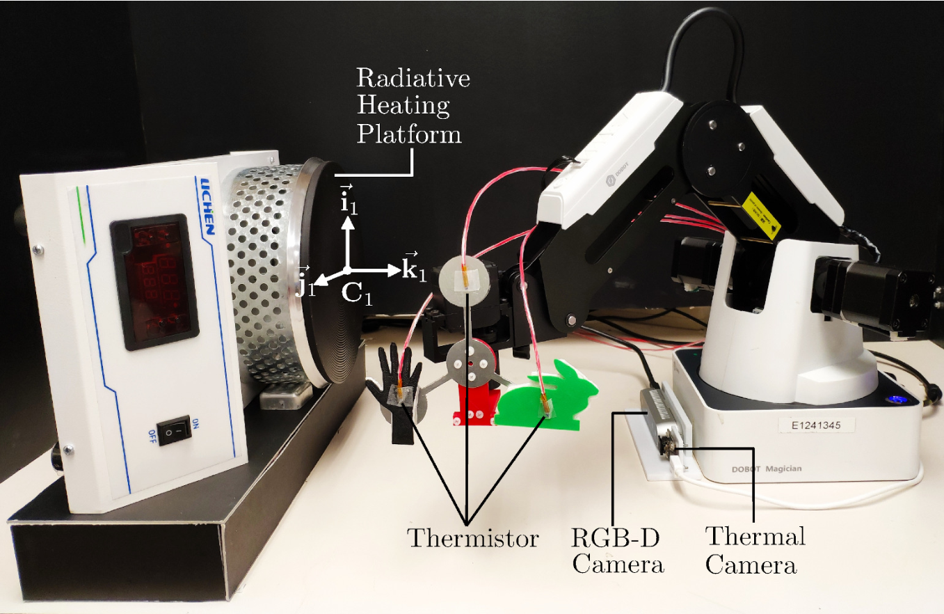
We conducted a series of experiments on a 4-DOF robot (3 translations and 1 rotation) to evaluate the proposed method. Fig. 8 shows the robot, whose end-effector is replaced by a 3D printed connector fixed to an aluminum holder. The objects are attached to the holder through an adiabatic layer to minimize heat conduction. We prepared three different kinds of objects for temperature control experiments (see Fig. 9): An aluminum circular sheet with $1.5\text{\,}\mathrm{cm}$ radius and $3\text{\,}\mathrm{mm}$ thickness; A bunny-shaped object with $1\text{\,}\mathrm{mm}$ thickness, 3D printed using polylactic acid (PLA) material with $30\%$ infill density; A hand-shaped sheet with $1\text{\,}\mathrm{mm}$ thickness, also 3D printed using PLA but with $50\%$ infill density. We approximate the aluminum sheet’s and the heat source’s thermophysical properties via standard tables [29]. The object’s emittance, absorptance, specific heat, and density are 0.04, 0.04, $903\text{\,}\mathrm{J}\text{$\cdot$}{\mathrm{K}}^{-1}\text{$\cdot$}{\mathrm{kg}}^{-1}$, and $2702\text{\,}\mathrm{kg}\text{$\cdot$}{\mathrm{m}}^{-1}$, respectively. The source’s emittance and absorptance are estimated as 0.25 and 0.25.

For the two 3D printed objects, different infill densities, colors, and uncertain surface conditions make their thermophysical properties hard to be estimated. Thus, we only consider the aluminum sheet for the experiments with the model-based controller (adaptive control is used for the other objects). A radiative heating platform with adjustable temperature output is used as the heat source. The (indoor) environment temperature is assumed to be constant at $23\text{\,}\mathrm{\SIUnitSymbolCelsius}$.

To obtain the feedback temperatures, we attach a PT100 platinum thermistor with $0.3\text{\,}\mathrm{\SIUnitSymbolCelsius}$ accuracy and $0.1\text{\,}\mathrm{\SIUnitSymbolCelsius}$ precision to each object. The raw data obtained by thermistors is processed by a current-temperature transformation module and sent to a Linux-based control computer as the feedback signal. The motion command is calculated by the computer program and sent to the robot under a position-stepping mode. At the beginning of the experiments, we use an RGB camera and three ArUco markers [47] to calibrate the configuration between the heat source and the end-effector (see Fig. 10).

We conduct a series of thermal servoing experiments to evaluate our proposed control methodology (see Fig. 11 for a representative experiment). Here, we first evaluate the performance of the model-based controller with aluminum objects (whose properties are approximately known); The experiments are conducted with a source’s temperature of $200\text{\,}\mathrm{\SIUnitSymbolCelsius}$.

We denote the scalar temperature error by $\Delta T=T_{2}-T^{*}$. By using the controller (35), we enforce a closed-loop heat transfer system that resembles a mass-spring-damper system. Therefore, the values of the stiffness/damping-like gains $K$ and $D$ can be used to specify the system’s performance. Fig. 12 (a) demonstrates the effect of the gain $K$ on the thermal response. For that, we set $D=0.2$ and $T^{*}=$50\text{\,}\mathrm{\SIUnitSymbolCelsius}$$ and conduct three experiments with different $K$ values. These show that when $K=0.005$ (red curve), the error $\Delta T$ asymptotically decreases to zero with a relatively slow speed; When $K=0.05$ (blue curve), $\Delta T$ decreases faster and a small overshoot occurs; When $K=0.5$ (black curve), $\Delta T$ oscillates near zero with an approximate $3\text{\,}\mathrm{\SIUnitSymbolCelsius}$ amplitude. This results shows how the closed-loop system varies from over-damped to under-damped. Thus, the gains should be specified according to the desired thermodynamic performance. We further conducted experiments with the same gains ($K=0.05$, $D=0.2$) but with different targets $T^{*}$ and found a consistent response (see Fig. 12 (b)).

Model-based experiments were also conducted to independently regulate the temperatures of two aluminum objects, shown in Fig. 9 (b). We designed 4 experiments with different targets $\boldsymbol{\tau}^{*}$ (measured in $\text{\,}\mathrm{\SIUnitSymbolCelsius}$). Fig. 13 depicts the minimization of the thermal errors for these 4 experiments, with target temperatures defined as $\boldsymbol{\tau}^{*}=[{50},{40}{]}^{{\hskip 0.0pt\intercal}}$, $\boldsymbol{\tau}^{*}=[{60},{40}{]}^{{\hskip 0.0pt\intercal}}$, $\boldsymbol{\tau}^{*}=[{50},{50}{]}^{{\hskip 0.0pt\intercal}}$, and $\boldsymbol{\tau}^{*}=[{80},{40}{]}^{{\hskip 0.0pt\intercal}}$ in (a), (b), (c), and (d), respectively. For the first three experiments where the differences between the target temperatures $|T^{*1}-T^{*2}|$ are small (or null), the thermal error $\|\Delta\boldsymbol{\tau}\|$ can be asymptotically minimized to zero. However, when $|T^{*1}-T^{*2}|$ is large, as in Fig. 13 (d), the two temperatures cannot be accurately controlled. This failure case can be explained by the second condition for feasible targets discussed in Section III-C.

We designed a series of experiments to evaluate the performance of the proposed adaptive controller. For that, we consider with three different objects (see Fig. 9 (c)) with unknown thermophysical properties and irregular shapes. To compute the interaction matrix, we use truncated Fourier series with 5 harmonics terms; This approach provides a fast calculation time with a “good enough” shape approximation. The controller’s gains are set to $\mu=0.05$ and $K=0.15$. To initialize the parameters $\widehat{\mathbf{a}}_{i}(0)$ at the time instance $t=0$, we use (for the “hand” and “bunny” objects) the constant values calculated for the aluminum object in the previous model-based controller, i.e. $\widehat{\mathbf{a}}_{i}(0)=\mathbf{a}_{i}$; For the circular object, we simply initialize $\widehat{\mathbf{a}}_{i}(0)$ with random values.

In this study, we report eight temperature control experiments with different targets, objects and source conditions. Figure 14 shows the evolution of the individual thermal errors $\Delta T^{i}$. For ease of presentation, we name these eight experiments as exp 1, …, exp 8, and denote the corresponding target temperature for each experiment by $\boldsymbol{\tau}^{*1},\ldots,\boldsymbol{\tau}^{*8}$. In exp 1, we set the three target temperatures to the same value. In exp 2 – exp 4, we only set two targets to the same value. In exp 5 and exp 6, we set all targets to different values, with a non-uniform thermal separated in exp 5 and a uniform one in exp 6. In exp 7 and exp 8, all targets are set to the same value, but with different heat source conditions. The source temperature $T_{1}$ is set to $200\text{\,}\mathrm{\SIUnitSymbolCelsius}$ in exp 1 – exp 6, to $300\text{\,}\mathrm{\SIUnitSymbolCelsius}$ in exp 7, and varies from $200\text{\,}\mathrm{\SIUnitSymbolCelsius}$ to $300\text{\,}\mathrm{\SIUnitSymbolCelsius}$ in exp 8.

References

- [1] D. Navarro-Alarcon, Y.-H. Liu, J. G. Romero, and P. Li, “On the visual deformation servoing of compliant objects: Uncalibrated control methods and experiments,” Int. Journal of Robotics Research, vol. 33, no. 11, pp. 1462–1480, 2014.
- [2] A. Cherubini and F. Chaumette, “Visual navigation of a mobile robot with laser-based collision avoidance,” Int. Journal of Robotics Research, vol. 32, no. 2, pp. 189–205, 2013.
- [3] M. Tirindelli, M. Victorova, J. Esteban, S. T. Kim, D. Navarro-Alarcon, et al., “Force-ultrasound fusion: Bringing spine robotic-us to the next “level”,” IEEE Robot. Autom. Lett., vol. 5, no. 4, pp. 5661–5668, 2020.
- [4] A. Magassouba, N. Bertin, and F. Chaumette, “Audio-based robot control from interchannel level difference and absolute sound energy,” in Proc. IEEE Int. Conf. Intelligent Robots and Systems, 2016, pp. 1992–1999.
- [5] F. Rahbar, A. Marjovi, P. Kibleur, and A. Martinoli, “A 3-d bio-inspired odor source localization and its validation in realistic environmental conditions,” in IEEE/RSJ Int. Conf. on Intelligent Robots and Systems, 2017, pp. 3983–3989.
- [6] R. Gade and T. B. Moeslund, “Thermal cameras and applications: A survey,” Machine Vision and Applications, vol. 25, pp. 245–262, 2014.
- [7] E. Benli, R. L. Spidalieri, and Y. Motai, “Thermal multisensor fusion for collaborative robotics,” IEEE Transactions on Industrial Informatics, vol. 15, no. 7, pp. 3784–3795, 2019.
- [8] Y. Cao, B. Xu, Z. Ye, J. Yang, Y. Cao, et al., “Depth and thermal sensor fusion to enhance 3d thermographic reconstruction,” Opt. Express, vol. 26, no. 7, pp. 8179–8193, Apr 2018.
- [9] Y. He and R. Yang, “Eddy current volume heating thermography and phase analysis for imaging characterization of interface delamination in cfrp,” IEEE Trans. on Industrial Informatics, vol. 11, no. 6, pp. 1287–1297, 2015.
- [10] W. W.-L. Lai, K.-K. Lee, and C.-S. Poon, “Validation of size estimation of debonds in external wall’s composite finishes via passive infrared thermography and a gradient algorithm,” Construction and Building Materials, vol. 87, pp. 113 – 124, 2015.
- [11] A. Cherubini and D. Navarro-Alarcon, “Sensor-based control for human-robot collaboration: Fundamentals, challenges and opportunities,” Front. in Neurorobotics (in press), vol. 1, no. 1, pp. 1–21, 2020.
- [12] W. Binrui, J. Yinglian, X. Hong, and W. Ling, “Temperature control of pem fuel cell stack application on robot using fuzzy incremental pid,” in 2009 Chinese Control and Decision Conference. IEEE, 2009, pp. 3293–3297.
- [13] M. Ho and J. P. Desai, “Towards a mri-compatible meso-scale sma-actuated robot using pwm control,” in 2010 3rd IEEE RAS & EMBS International Conference on Biomedical Robotics and Biomechatronics. IEEE, 2010, pp. 361–366.
- [14] J. De Backer, G. Bolmsjö, and A.-K. Christiansson, “Temperature control of robotic friction stir welding using the thermoelectric effect,” The International Journal of Advanced Manufacturing Technology, vol. 70, no. 1-4, pp. 375–383, 2014.
- [15] J.-H. Kim and B. Y. Lattimer, “Real-time probabilistic classification of fire and smoke using thermal imagery for intelligent firefighting robot,” Fire Safety Journal, vol. 72, pp. 40–49, 2015.
- [16] A. Cammarata, “Optimized design of a large-workspace 2-dof parallel robot for solar tracking systems,” Mechanism and machine theory, vol. 83, pp. 175–186, 2015.
- [17] M. Muddassir, D. Gomez, L. Hu, S. Chen, and D. Navarro-Alarcon, “Robotics meets cosmetic dermatology: Development of a novel vision-guided system for skin photo-rejuvenation,” IEEE/ASME Trans. Mechatronics (under review), vol. 1, no. 1, pp. 1–15, 2020.
- [18] D. McKemy, “Temperature sensing across species,” Eur. J. Physiol., vol. 454, pp. 777–791, 2007.
- [19] J. Mlynek, R. Knobloch, and R. Srb, “Optimization of a heat radiation intensity and temperature field on the mould surface.” in ECMS, 2016, pp. 425–431.
- [20] A. Imdoukh, A. Shaker, A. Al-Toukhy, D. Kablaoui, and M. El-Abd, “Semi-autonomous indoor firefighting uav,” in Int. Conf. on Advanced Robotics, 2017, pp. 310–315.
- [21] G. Muscato, F. Bonaccorso, L. Cantelli, D. Longo, and C. D. Melita, “Volcanic environments: Robots for exploration and measurement,” IEEE Robotics & Automation Magazine, vol. 19, no. 1, pp. 40–49, 2012.
- [22] M. Fu, W. Weng, W. Chen, and N. Luo, “Review on modeling heat transfer and thermoregulatory responses in human body,” Journal of Thermal Biology, vol. 62, pp. 189 – 200, 2016, modeling bioheat transfer processes and thermoregulatory responses.
- [23] R. Lee, “Thermal tolerances of deep-sea hydrothermal vent animals from the northeast pacific,” Biological Bulletin, vol. 205, no. 2, pp. 98–101, 2003.
- [24] C.-C. Tsai, R. A. Childers, N. N. Shi, C. Ren, J. N. Pelaez, et al., “Physical and behavioral adaptations to prevent overheating of the living wings of butterflies,” Nature communications, vol. 11, no. 1, pp. 1–14, 2020.
- [25] M. L. May, “Insect thermoregulation,” Annual review of entomology, vol. 24, no. 1, pp. 313–349, 1979.
- [26] L. Natale, G. Metta, and G. Sandini, “Development of auditory-evoked reflexes: Visuo-acoustic cues integration in a binocular head,” Rob. Auton. Syst., vol. 39, no. 2, pp. 87 – 106, 2002.
- [27] G. Arechavaleta, J. Laumond, H. Hicheur, and A. Berthoz, “An optimality principle governing human walking,” IEEE Trans. Robot., vol. 24, no. 1, pp. 5–14, 2008.
- [28] S. Na, Y. Qiu, A. E. Turgut, J. Ulrich, T. Krajník, et al., “Bio-inspired artificial pheromone system for swarm robotics applications,” Adaptive Behavior, pp. 1–21, 2020.
- [29] T. L. Bergman, F. P. Incropera, D. P. DeWitt, and A. S. Lavine, Fundamentals of heat and mass transfer. John Wiley & Sons, 2011.
- [30] M. F. Modest, Radiative heat transfer. Academic press, 2013.
- [31] I. Lienhard and H. John, A heat transfer textbook. phlogiston press, 2005.
- [32] M. Vujičić, N. Lavery, and S. Brown, “View factor calculation using the monte carlo method and numerical sensitivity,” Communications in numerical methods in Engineering, vol. 22, no. 3, pp. 197–203, 2006.
- [33] J. C. Chai, J. P. Moder, and K. C. Karki, “A procedure for view factor calculation using the finite-volume method,” Numerical Heat Transfer: Part B: Fundamentals, vol. 40, no. 1, pp. 23–35, 2001.
- [34] S. C. Mishra, A. Shukla, and V. Yadav, “View factor calculation in the 2-d geometries using the collapsed dimension method,” International communications in heat and mass transfer, vol. 35, no. 5, pp. 630–636, 2008.
- [35] M. Vujičić, N. Lavery, and S. Brown, “Numerical sensitivity and view factor calculation using the monte carlo method,” Proceedings of the Institution of Mechanical Engineers, Part C: Journal of Mechanical Engineering Science, vol. 220, no. 5, pp. 697–702, 2006.
- [36] E. M. Sparrow, Radiation heat transfer. Routledge, 2018.
- [37] V. R. Rao and V. Sastri, “Efficient evaluation of diffuse view factors for radiation,” International journal of heat and mass transfer, vol. 39, no. 6, pp. 1281–1286, 1996.
- [38] H. Flanders, “Differentiation under the integral sign,” The American Mathematical Monthly, vol. 80, no. 6, pp. 615–627, 1973.
- [39] P. Virtanen, R. Gommers, T. E. Oliphant, M. Haberland, T. Reddy, et al., “SciPy 1.0: Fundamental Algorithms for Scientific Computing in Python,” Nature Methods, vol. 17, pp. 261–272, 2020.
- [40] G. P. Tolstov, Fourier series. Courier Corporation, 2012.
- [41] D. Navarro-Alarcon and Y.-H. Liu, “Fourier-based shape servoing: a new feedback method to actively deform soft objects into desired 2-d image contours,” IEEE Transactions on Robotics, vol. 34, no. 1, pp. 272–279, 2018.
- [42] T. Muneer, S. Ivanova, Y. Kotak, and M. Gul, “Finite-element view-factor computations for radiant energy exchanges,” Journal of Renewable and Sustainable Energy, vol. 7, no. 3, p. 033108, 2015.
- [43] Y. Nakamura, Advanced robotics: redundancy and optimization. Boston, MA: Addison-Wesley Longman, 1991.
- [44] M. Vidyasagar, Nonlinear systems analysis. SIAM, 2002.
- [45] N. Titchener, S. Colliss, and H. Babinsky, “On the calculation of boundary-layer parameters from discrete data,” Experiments in Fluids, vol. 56, no. 8, p. 159, 2015.
- [46] Y.-H. Liu, H. Wang, C. Wang, and K. K. Lam, “Uncalibrated visual servoing of robots using a depth-independent interaction matrix,” IEEE Trans. Robot., vol. 22, no. 4, pp. 804–817, Aug. 2006.
- [47] S. Garrido-Jurado, R. Muñoz-Salinas, F. J. Madrid-Cuevas, and M. J. Marín-Jiménez, “Automatic generation and detection of highly reliable fiducial markers under occlusion,” Pattern Recognition, vol. 47, no. 6, pp. 2280–2292, 2014.
- [48] D. Navarro-Alarcon, J. Qi, J. Zhu, and A. Cherubini, “A Lyapunov-stable adaptive method to approximate sensorimotor models for sensor-based control,” Front. in Neurorobotics, vol. 14, no. 59, pp. 1–12, 2020.
- [49] C. Williams, “Research methods,” Journal of Business & Economics Research (JBER), vol. 5, no. 3, 2007.
- [50] D. Hai and R. Smith, “An elementary proof of the error estimates in simpson’s rule,” Mathematics Magazine, vol. 81, no. 4, pp. 295–300, 2008.
![[Uncaptioned image]](2012.13147v1/luyin.png) |
Luyin Hu received his BEng. degree in Mechanical Engineering from The Hong Kong Polytechnic University, KLN, Hong Kong in 2019. Currently, he is pursuing an MPhil degree in Mechanical Engineering at the same university, where he also works as a Research Assistant. His research interests include multimodal robot perception, servomechanisms, and control system design. |
![[Uncaptioned image]](2012.13147v1/david.png) |
David Navarro-Alarcon (GS’06–M’14–SM’19) received the Ph.D. degree in Mechanical and Automation Engineering from The Chinese University of Hong Kong (CUHK), Shatin, Hong Kong, in 2014. He was an Assistant (Research) Professor at the CUHK T Stone Robotics Institute, from 2015 to 2017. Since 2017, he has been with The Hong Kong Polytechnic University, KLN, Hong Kong, where he is an Assistant Professor at the Department of Mechanical Engineering. His current research interests include perceptual robotics and control theory. |
![[Uncaptioned image]](2012.13147v1/andrea.png) |
Andrea Cherubini received the M.Sc. in Mechanical Engineering in 2001 from the University of Rome La Sapienza and a second M.Sc. in Control Systems in 2003 from the University of Sheffield, U.K. In 2008, he received the Ph.D. in Control Systems from La Sapienza. From 2008 to 2011, he was postdoc at INRIA Rennes. Since 2011, he is Associate Professor at Université de Montpellier. His research interests include: physical human–robot interaction, and manipulation of soft objects. |
![[Uncaptioned image]](2012.13147v1/mengying.png) |
Mengying Li received her PhD degree in Mechanical and Aerospace Engineering from University of California San Diego. From 2018 to 2020, She was a Postdoctoral Scholar in the Center for Energy Research of UC San Diego. She joined The Hong Kong Polytechnic University as an Assistant Professor in the Department of Mechanical Engineering since 2020. Her research interests include atmospheric radiative heat transfer for renewable energy integration and design of multi-generation systems. |