∎
Kryging: Geostatistical analysis of large-scale datasets using Krylov subspace methodsJournal: Statistics and Computing
Abstract
Analyzing massive spatial datasets using a Gaussian process model poses computational challenges. This is a problem prevailing heavily in applications such as environmental modeling, ecology, forestry and environmental health. We present a novel approximate inference methodology that uses profile likelihood and Krylov subspace methods to estimate the spatial covariance parameters and makes spatial predictions with uncertainty quantification for point-referenced spatial data. The proposed method, Kryging, applies for both observations on regular grid and irregularly-spaced observations, and for any Gaussian process with a stationary isotropic (and certain geometrically anisotropic) covariance function, including the popular Matrn covariance family. We make use of the block Toeplitz structure with Toeplitz blocks of the covariance matrix and use fast Fourier transform methods to bypass the computational and memory bottlenecks of approximating log-determinant and matrix-vector products. We perform extensive simulation studies to show the effectiveness of our model by varying sample sizes, spatial parameter values and sampling designs. A real data application is also performed on a dataset consisting of land surface temperature readings taken by the MODIS satellite. Compared to existing methods, the proposed method performs satisfactorily with much less computation time and better scalability.
Keywords:
Approximate inference Profile likelihood Block Toeplitz matrix Fast Fourier transform Krylov subspace methods Golub-Kahan bidiagonalization1 Introduction
Massive spatial datasets, often coming from satellites or other remotely-sensed sources, have become increasingly common in applications such as environmental health, forestry, ecology etc. Classical geostatistical analysis methods for point-referenced spatial data are burdened with computationally intensive steps such as Cholesky factorization or eigendecomposition which have cubic complexity in the number of observations. Despite the advances in computing performance, these methods remain prohibitively expensive to apply to datasets of even moderately-large size. Therefore, we need to develop methods that perform nearly as well as the classical methods but are more computationally efficient and therefore applicable to problems of massive volume.
There is a rich literature of approximate inference methods for point-referenced spatial data. Early approaches approximated the joint likelihood by decomposing it into a product of conditional distributions (Vecchia 1988; Stein et al. 2004), using pseudo-likelihood (Varin et al. 2011; Eidsvik et al. 2014) or using covariance tapering (Furrer et al. 2006; Kaufman et al. 2008; Stein 2013). Modeling in the spectral domain (Fuentes 2007; Guinness and Fuentes 2017; Guinness 2019) was also used to circumvent the heavy computation. Another class of approaches are based on finite-rank approximations such as fixed-rank Kriging (Cressie and Johannesson 2008; Kang and Cressie 2011; Katzfuss and Cressie 2011), predictive process (Banerjee et al. 2008; Finley et al. 2009), process convolution (Higdon 2002) and lattice Kriging (Nychka et al. 2015). Other approaches use a combination of hierarchical matrix approaches and stochastic estimators for the log-likelihood (Anitescu et al. 2012; Ambikasaran et al. 2015; Minden et al. 2017; Eriksson et al. 2018; Stein 2013) or spectral methods and h-likelihood (Dutta and Mondal 2016).
More recent approaches make use of the modern computing platforms and focus on parallelizing the computational load. Paciorek et al. 2015 is one such example. Katzfuss 2017 and Katzfuss and Hammerling 2017 combine low rank methods with distributed computing. Dividing the data into subsets, drawing inference on these subsets in parallel and recombining them has been proposed by Barbian and Assunção 2017 and Guhaniyogi and Banerjee 2018. Datta et al. 2016a; Datta et al. 2016b; Datta et al. 2016c use an approximation based on the conditional distribution given the nearest neighbors, inducing sparsity and allowing the method to be parallelized. The stochastic partial differential equation or SPDE (Lindgren et al. 2011) approach induces sparsity in the inverse-covariance matrix for fast approximations. Sun et al. 2012, Bradley et al. 2016, Heaton et al. 2019 and Liu et al. 2020 provide comprehensive reviews of these methods and demonstrate their effectiveness in spatial modeling.
Most of these methods use either finite-rank approximations or introduce sparsity in the covariance or the inverse-covariance structure. Finite rank based models typically have complexity with being the rank of the model such that . However, in order for the approximation to be effective for large , a large rank is needed which increases the computational costs. This cost can be alleviated by inducing sparsity into the covariance structure using compactly supported covariance function; however, this may not be an appropriate modeling choice when long-range dependence is present in the data.
We present a novel statistical method of log-linear complexity to provide approximate inference for massive geostatistical datasets using profile maximum likelihood estimation and Krylov subspace methods based on the genHyBR method proposed by Chung et al. 2018. The proposed method, Kryging, provides prediction for the observed process at unobserved locations by approximating the underlying spatial process on a regular, equispaced grid. Although we approximate the latent process on a grid, we do not restrict the observations to be on grid and therefore the method can be applied to irregularly-spaced large spatial datasets. We generate estimates of the underlying process through Krylov subspace methods. Krylov subspaces (See Saad 2003, for reference) are efficient iterative methods for solving large-scale linear systems and least squares problems. A key advantage of the Krylov subspace approach is that it is matrix-free, in that it does not require forming the matrices explicitly, but only requires the action of the matrix on appropriate vectors. We provide prediction uncertainty estimates in the form of pointwise confidence intervals via a parametric bootstrap approach and estimates for the mean and spatial covariance parameters. Kryging applies to any stationary isotropic covariance structure, e.g., the Matérn covariance family, as well as covariance functions that incorporate geometric anisotropy by allowing dissimilar stretching along the two axes. It exploits the Toeplitz (in one dimension) or block Toeplitz with Toeplitz blocks (BTTB) structure (in higher dimensions) of the resulting covariance matrices and employs a fast Fourier transformation based method for achieving computational gains for matrix-vector multiplications (Gray 2006, See ) and approximating log-determinants (Kent and Mardia 1996). As a result, Kryging has storage costs and only computational complexity where is the size of the underlying grid for estimating the spatial parameters and performing spatial prediction.
The tools used for building the Kryging model have been used in literature before in different contexts and different problems. However, by efficiently combining them in a specific manner, Kryging has several advantages compared to related methods in the literature. Chung et al. 2018 also use the same core method but we extend it to include mean and spatial covariance parameter estimation, uncertainty quantification and approximation of log-determinants. Aune et al. 2014 and Dutta and Mondal 2016 also use tools such as Krylov subspaces and the fast Fourier transformation, but their usage differs vastly from ours. First, we construct a different Krylov subspace, one that incorporates the noise covariance, a mapping matrix, and the covariance matrix; in contrast, the approach in the other papers is to build a Krylov subspace method with the covariance matrix alone. Second, we use the Golub-Kahan bidiagonalization rather than Lanczos or Conjugate Gradient for linear systems. Third, we use the basis vectors from the Krylov subspace to estimate the objective function and the gradients (one exception is the determinant and its derivative for which we use a different approximation). In contrast, other approaches use various tools such as Monte Carlo trace estimators, to estimate the various quantities.
Kryging has a low-rank matrix involved in the approximation process. However, compared to other low-rank methods discussed above, empirical evidence hints that using a small order of the Krylov subspace works well for huge datasets and produces accurate results. Block-circulant embeddings has been proposed as a stand-alone method to approximate determinants (Rue and Held 2005) which nicely gels with the Krylov subspace based approximation to the problem of maximizing the quadratic part of a Gaussian log-likelihood to produce a fast and scalabe approximate inference method for massive geostatistical datasets.
We establish the particular form of latent Gaussian model that we use for our method in Section 2. Section 3 gives the details of the method. We provide detailed description and algorithms of components of the method in various subsections of Section 3. A thorough simulation study is performed in Section 4 and an application to MODIS satellite data is performed in Section 5. The data analysis is based on Heaton et al. 2019. The rationale behind this was to be able to compare the performance of our method to other available methods directly. We finish with a discussion and concluding remarks in Section 6.
2 Latent Gaussian Model
Let be the observed process and is the underlying process of interest at location , ; throughout this paper, we illustrate the methods using the but our approach is applicable to problems with two or three spatial dimensions with a possible additional time dimension. A realization from the observation process, , at locations is related to a realization from the latent process, , at possibly different locations by the relationship
| (1) |
where with being a cheaply invertible matrix of individual variances for each location, being the matrix of corresponding covariates observed at the same locations as the observations themselves and being a matrix that specifies the linear combinations that connect the mean removed and . For this paper, we make the standard assumption that the nugget variance is constant across space and set .
The mapping matrix permits the flexibility of and not being co-located, as well as change of support. For example, , the identity matrix, represents the case where is a noisy observation of itself after accounting for the mean process. In case the response locations are a subset of the locations , then is the identity matrix with rows removed. The matrix can be non-diagonal as well, for the case when value of at each location is considered as an average of the unobserved at nearby locations, as it can be when is observed at locations at irregularly spaced locations and is considered on a grid around those locations.
When the observations are not on a regular grid, we still set the latent process locations to be on a rectangular grid and account for the irregularity of the observation locations in the mapping matrix, . We specify the entries of so that each observation is a convex combination of the latent process in the neighborhood of the observation. Specifically, the latent process is weighted by the Wendland kernel function (Wendland 1995) , where and , and are the grid spacings in the two directions and and are the -th observation location and -th grid-point location, respectively. This particular formulation allows to approximate the value at a point outside of the grid as a weighted combination of its nearest four neighbors while for a point on the grid itself, the approximation is exact. To ensure the weights are convex, they are normalized to sum to one for each observation. That is, we assume the mean response is
This is equivalent to setting the element of to . The truncation function ensures that is a sparse matrix with at most four nonzero entries per row, i.e., the matrix has nonzero entries.
Choosing the mapping matrix to be sparse ensures there is not significantly higher computational cost due to these changes when applying to an irregularly spaced data. This approach to handling irregularly-spaced observations introduces an additional tuning parameter, , which controls the density of the latent space observations. When the observation locations are on a regular grid, we simply set it to be equal to so that the latent process locations match the observations. However, when the observations are not on a grid then there is no natural choice for . Accuracy should increase with at the expense of computational burden. This issue is explored further in the simulation study of Section 4.
We use a latent Gaussian process to model the true state , with zero mean and isotropic Matrn covariance kernel (Matérn 1960) with standard deviation , spatial range parameter and smoothness parameter . Therefore, at finite collection of locations, is a multivariate Gaussian distribution with mean and correlation matrix , i.e.,
| (2) |
with being the vector of all zeros and
being the spatial correlation between locations and induced by the stationary isotropic Matrn covariance kernel for . Here and denotes the Euclidean norm in and is the modified Bessel function of the second kind with parameter . The choice of Matrn covariance kernel is common but any other stationary covariance function (or geometrically anisotropic covariance function that induces different stretching along the two axes) may be used along with the approach for both regularly gridded and irregularly spaced datasets with same computational complexity that we outline in the next section.
3 Inferential Approach
In this section, we describe an inferential approach for the latent Gaussian model that combines Kriging and Krylov subspace methods, which we have been calling “Kryging”. The likelihood function for the latent state and the mean and spatial variance parameters can be written as
| (3) |
where is the density of the data given and is the density of ; both densities depend on the parameter . Since we assumed a Gaussian model for and , we have
where means equal up to a constant that is unimportant for the purposes of optimization and and
| (4) |
Thus the log-likelihood function, has the form
| (5) |
Evaluation of the log-likelihood function involves inverting and computing the log-determinant of the covariance matrix , both of which require many operations which is not feasible for large . Since the optimization needs to run on both and , it would be a ultra high-dimensional optimization which would generally be infeasible to implement. Therefore, running an optimization procedure over both and on this objective function straightaway is futile and we must look into approximation methods to avoid these computational bottlenecks.
We propose a computationally-efficient inference approach using approximate inference for fast estimation for both parameters and the underlying true state variables along with its uncertainty. We profile as a function of the parameters and maximize the corresponding profile likelihood over (Cox and Snell 1989). This reduces the dimensionality of the optimization problem greatly but it requires an estimate of for a given value of .
The genHyBR method (Chung et al. 2018) circumvents the matrix inversion problem as it brings down the total complexity of computing the quadratic term to that of a matrix vector multiplication. Typically this would take operations. However, computational techniques such as Fast Fourier Transforms (FFTs) or -matrices (a review of techniques can be found in Ambikasaran et al. 2015) can reduce the computational cost of storage and the mathematical operators to , where is a non-negative exponent which depends on the operation and the method used. In particular, we use the symmetric BTTB structure of . The symmetric BTTB structure allows us to store in , since only one row/column of needs to be stored, and compute the matrix vector products involving in time. If the underlying process realizations are not on a regular grid, then the -matrix approach can be used instead with the same computational cost. However, with the mapping matrix strategy laid out in Section 2, we do not require this approach. The symmetric BTTB structure also allows us to compute the log-determinant of in time. This gives us a good estimate for for a given value of .
3.1 Profile Likelihood
Maximizing the log-likelihood function in Eq. (5) as a function of both and is not feasible and therefore we use a profile likelihood based optimization strategy by profiling as a function of . Profiling out from Eq. (5) as a function of , in exact arithmetic, results in
| (6) |
Plugging in in Eq. (5) and calling produces the exact profile log-likelihood function
| (7) |
Since simply evaluating this function involves computing inverses and determinants of the dense covariance matrix, it must be approximated.
Evaluating the exact profile likelihood presents three computational challenges: (1) computing involves inverting large dense matrices, (2) computing the quadratic term and (3) computing the log-determinant of . The first two are overcome using the genHyBR method (Chung et al. 2018) while the log-determinant term is approximated using the symmetric BTTB structure of the resulting covariance matrix from the choice of appropriate covariance function previously mentioned in Section 2. Once these approximations are in place, optimization of an approximated profile likelihood function can be performed using typical optimization routines to get the estimates of and .
3.2 genHyBR Method
A key component in maximizing the profile likelihood is to quickly compute for a given . The computation of in this context is tantamount to computing
| (8) |
where and represents the Euclidean norm. The genHyBR algorithm (Chung et al. 2018) solves this weighted least squares problem iteratively using generalized Golub-Kahan bidiagonalization which is a special type of Krylov subspace method (Benbow 1999; Chung and Saibaba 2017). To simplify notation, we drop the dependence on and write .
We provide an outline of the algorithm here. Denote as the Krylov subspace of degree . Observing that Eq. (8) involves the inverse of , employing a change of variables and , we then compute and
| (9) |
Then, for our problem of estimating , the genHyBR method (Chung et al. 2018) looks for the solution of in
The genHyBR algorithm creates an basis for this subspace, i.e., using an efficient Golub-Kahan bidiagonalization iteration scheme which has been sketched in Algorithm 1.
From Algorithm 1, we also obtain a bidiagonal matrix
The outputs of the algorithms satisfy the following relationships
| (10) |
Since we are looking for a solution of , we can write and determine by solving
| (11) |
Therefore, given and and by undoing the change of variables, we approximate the solution to Eq. (8) as
| (12) |
where is the first column of the identity matrix; that is, the vector with the first entry and every other entry equal to . In general, a stopping criterion must be used to terminate the iterations and to automatically determine the number of iterations . Details on one such choice of stopping criterion are given in Chung et al. 2018. However, we do not use the said criterion for our method and instead treat the parameter as an algorithm parameter to be input by the user. The orthogonal basis vectors and may not remain numerically orthogonal and therefore may require a reorthogonalization scheme. Such a scheme is described in the Chung et al. 2018 paper and is available for the user to use in Kryging as well. However, we do not use it for the results presented in this paper.
The genHyBR method reduces the computational complexity of solving for from to that of matrix vector multiplication, . When the latent process locations are arranged on a rectangular grid, is symmetric BTTB and thus the matrix-vector multiplication can be achieved swiftly, in flops, using circulant embedding. Additionally, due to the form of in Eq. (12) and the exact arithmetic relationships presented in Eq. (10), the quadratic term can now be approximated as , where . This requires only operations.
3.3 Log-determinant Approximation
To compute the determinant of , we once again use the symmetric BTTB structure of . Gray 2006 reviews methods for creating a circulant matrix based on a Toeplitz matrix and using the circulant matrix structure to approximate the determinant of a Toeplitz matrix using inverse FFTs. Refer to Section and of Gray 2006 for details. This behavior can be extended to a BTTB structure as well and a similar asymptotic result also holds for them (Gyires 1956; Widom 1974). The block circulant matrix can be created exactly as it is done for circulant embedding based matrix-vector product and therefore does not add any extra computation. The approximation to the log-determinant is of the form
where .
The approximation stems from the fact that the result is only exact in an asymptotic sense. However, numerical evidence suggests that the approximation to the determinant and its derivatives improves as the number of grid points increases; a more precise statement of convergence can be found in Theorem 1.1 and Lemma 4.1(b) of Kent and Mardia 1996. We mention that besides the BCCB approximation, there are other ways of estimating the log-determinant, such as stochastic trace estimation (Anitescu et al. 2012; Ubaru et al. 2017) and using Hierarchical matrix structure (Ambikasaran et al. 2015; Minden et al. 2017). In particular, the advantage of the stochastic trace estimator is that the information used in estimating the log-determinant can be reutilized during the computation of the gradient information. These approaches can be used in place of the proposed estimator.
3.4 Optimization Details
The approximations described in the previous sections render the approximate profile log-likelihood function to have the form
| (13) |
where , and are as described in Section 3.2 and is as described in Section 3.3. Evaluating this function is faster and we can put it in an optimization routine to optimize over to get the estimates of and .
We use the MATLAB optimization routine fminunc with log-transformed range and variance parameters to avoid the non-negativity constrains. The optimization algorithm we use is a trust-region algorithm, which requires derivative information such as gradients and Hessians. The true gradient functions involve terms with and therefore needs to be approximated. These problems are averted by using the genHyBR solution of in place of as the matrix inversion problem reduces to a matrix vector multiplication problem. The derivative of the determinant is also approximated by using the BTTB structure. The details are given in Appendix A. To approximate the Hessian, we use a rank-one estimate of Hessian computed as the outer product of the approximate gradient. The rationale behind this approximation is the fact that, in expectation, the outer product of the score function equals the information matrix. Once again, the details are given in Appendix A.
3.5 Uncertainty Quantification
Besides a point estimate for , we also want to quantify the uncertainty associated with the estimated and the predicted . We employ a parametric bootstrap for uncertainty quantification. Using the estimated , we generate samples of from a zero-mean Gaussian process. For each , we generate from the model in Eq. (1) with and replaced by their estimates. We then estimate by Kryging, but assuming is known.
On the set of prediction locations , we compute the bootstrap MSE for each location as
| (14) |
This serves as an estimate of the classical Kriging variance for spatial prediction (Den Hertog et al. 2006). Since we use a parametric bootstrap approach, we use bootstrap samples as just this many bootstrap samples provide satisfactory performance. The entire scenario entails using genHyBR method (Chung et al. 2018) times, therefore costs flops. This procedure only approximates the uncertainty of the predictions assuming is known. However, the bootstrap could be extended to give standard errors for the elements of as well as prediction variances that account for uncertainty in by simply estimating for each bootstrap sample.
3.6 Summary of the Method
We now summarize the overall computational cost of this procedure. There are three main steps:
- 1.
Optimizing the profiled likelihood to obtain
- 2.
Compute and .
- 3.
Compute prediction variance using bootstrap sampling.
The optimization routine involves computing an approximate profile likelihood function and uses approximations based on the genGK algorithm to gradients and Hessian. Using genGK algorithm takes only steps for computing at the -th iteration of the optimization.
Caveat: Kryging depends on circulant embedding operations via the log-determinant approximation and bootstrap based uncertainty quantification. A successful execution requires that a positive definite embedding be found for the corresponding Gaussian process. Without this, the method may fail to produce a bootstrap sample from the Gaussian process in question and as a result fail to estimate uncertainty. This will also result in poor approximation of the log-determinant as many near-zero positive eigenvalues would be computed as near-zero negative eigenvalues and throw off the overall computation. This problem is evidently present when the spatial range parameter is high for the Gaussian process (Graham et al. 2018, See ). This problem with circulant embedding is well known. The problem of generating samples from a Gaussian process can be ameliorated by using different periodic embedding schemes (Stein 2002; Gneiting et al. 2006; Guinness and Fuentes 2017, See ). Forcefully resetting the small negative eigenvalues to zero or machine-precision value is a quick recourse for approximating the log-determinant. The different embedding schemes proposed in the literature may also be considered for this. However, none of these can solve the computational issue completely.
4 Simulation Studies
In this section, we perform simulation studies to evaluate the performance of our proposed method. These studies aim to demonstrate the effectiveness of the model with varying sample size as well as under different parametric settings for both gridded and irregularly spaced data. We perform three different simulation studies towards this goal. In each of the experiments, for each case, we repeat the process on 25 replications. Throughout the studies, the observed values are created by adding noise to , where is an observation from a Gaussian process with constant mean and exponential covariance function (i.e., Matrn covariance with ) with sill and spatial range . We take the variance of the noise process to be .
The first study varies the number of observations by generating data on a , , and grid in the unit square. The covariate matrix is a single column vector of ones and the choice of is taken to be . The Kryging method is fit using the same grid of used to generate the data and we compare performance for . About of the observed data were held out and were treated as test data upon which the performance was evaluated.
The second study demonstrates the performance of the method under different parametric settings on a grid of points. The spatial extents were kept same as in the first study. The four different parametric settings that were used for this study are as follows:
- 1.
Small spatial range, .
- 2.
Large spatial range, .
- 3.
Small partial sill, .
- 4.
Large partial sill, .
In all of these cases, about of the data from randomly chosen locations on the grid, were held out from the observed and kept as test sample data on which to evaluate the method.
The third study deals with the issue of irregularly spaced data. We used the first parametric setting, and the spatial extent of the data as in the first study.
The number of observed points were of which were held out as test samples. The data were generated by drawing on a grid and discarding of the data at random, leaving an irregularly spaced dataset of observations. For testing the scalability with the grid size , we used , and grids for .
The root mean squared error (RMSE) in predicting , pointwise coverage (CVG) of prediction intervals for these predictions were averaged over replications and median of computation time (MedTime) for all the replications were noted. These were used as performance metrics for each of the cases. For a competing method, we use the SPDE method available in the R package INLA. The SPDE method emerged from the comparison of several methods in Heaton et al. 2019 as one of the leading methods in terms of both computational speed and predictive accuracy.
a)
Grid Size
SPDE
Kryging
SE
k=20
k=50
k=100
k=200
0.910.95
0.930.92
0.910.91
0.910.91
0.910.91
0.030.03
0.830.95
0.860.92
0.840.91
0.830.91
0.830.91
0.010.02
0.800.95
0.860.92
0.840.91
0.830.91
0.830.91
0.010.02
0.780.95
0.840.91
0.800.89
0.790.88
0.780.88
0.010.02
b)
Grid Size SPDE Kryging k=20 k=50 k=100 k=200 5.42 (0.66) 0.14 (0.00) 1.84 (0.49) 5.14 (0.03) 11.00 (0.15) 44.64 (10.57) 5.51 (0.02) 1.66 (0.28) 2.12 (0.09) 48.24 (0.54) 170.01 (21.46) 3.39 (0.01) 4.11 (0.03) 5.49 (0.20) 7.81 (0.24) 662.95 (108.14) 10.78 (0.03) 12.02 (0.12) 14.28 (0.17) 18.09 (0.22)
Table 1 presents the RMSE and pointwise coverage values, averaged over replications, for the first simulation study and the median time for computation over the replicates for different choices of the tuning parameter and different grid sizes. In all cases, seems to be sufficient. The occasional inconsistencies in the computation times in Table 1 are due to the differences in the number of iterations taken by the optimization procedure to converge. In terms of RMSE and coverage, both the methods perform similarly but Kryging is considerably faster and is more scalable. On the other hand, the coverage for the proposed method is slightly below the nominal level. This may be due to ignoring uncertainty in when computing the prediction variances using Eq. 14. A possible fix for this is mentioned at the end of Section 3.5. However, the coverage is not so low as to require such a fix sacrificing its fast runtime advantage.
a)
Setting
SPDE
Kryging
SE
k=20
k=50
k=100
k=200
Setting 1
0.910.95
0.980.89
0.920.88
0.910.88
0.910.88
0.010.01
Setting 2
0.780.95
0.800.91
0.800.89
0.790.89
0.790.89
0.010.03
Setting 3
0.800.95
0.800.86
0.790.83
0.790.83
0.790.83
0.080.03
Setting 4
0.900.95
0.980.96
0.920.96
0.910.96
0.900.96
0.020.01
b)
Setting SPDE Kryging k=20 k=50 k=100 k=200 Setting 1 17.69 (2.63) 0.90 (0.00) 1.40 (0.08) 2.15 (0.10) 48.25 (0.47) Setting 2 19.03 (1.06) 5.56 (0.05) 1.60 (0.25) 2.12 (0.07) 48.74 (0.88) Setting 3 18.26 (3.10) 5.47 (0.41) 1.37 (0.08) 2.17 (0.08) 48.53 (0.27) Setting 4 18.49 (2.19) 5.57 (0.04) 2.37 (1.02) 2.16 (0.08) 48.62 (0.52)
The results for the grids with different true spatial covariance parameters are given in Table 2. For Settings 2 and 3, works well. This is not surprising for Setting 2 because the process with large range is smooth as easier to represent with a small number of terms. Solid performance for small in Setting 3 with lower partial sill is also expected because genHyBR (Chung et al. 2018) makes use of the partial sill to nugget ratio being moderate. As in the first simulation, going beyond seems unnecessary and the prediction RMSE performance is comparable to that of the SPDE method, but with substantially faster computation. Since INLA is implemented in R and Kryging is implemented in Matlab, the difference in platform makes the computing time comparisons difficult to interpret. However, the gain in computation time for Kryging is likely not the result of change in platform solely because INLA is highly optimized code (Martino and Rue 2009).
a)
Gridsize
SPDE
Kryging
SE
k=20
k=50
k=100
0.820.95
0.850.90
0.830.88
0.830.87
0.020.02
0.820.95
0.850.90
0.830.89
0.830.88
0.020.02
0.820.95
0.850.91
0.830.89
0.820.89
0.020.02
b)
Gridsize SPDE Kryging k=20 k=50 k=100 33.55 (3.58) 8.08 (0.02) 3.33 (0.31) 3.93 (0.15) 33.55 (3.58) 4.86 (0.02) 5.58 (0.03) 6.85 (0.05) 33.55 (3.58) 8.58 (0.10) 9.96 (0.11) 12.40 (0.09)
The results for irregularly-spaced data are shown in Table 3. The performance is similar to the SPDE method for the proposed method with slight undercoverage. In essence, the performance is quite similar to the regularly gridded data scenario in the first simulation study.
We also check the performance of the proposed method in estimating the true mean and spatial covariance parameters against those obtained from SPDE. Across all settings and irrespective of whether the data was on a regular grid or not, the results are consistent. While SPDE does a better job at estimating the nugget parameter, Kryging does a better job at estimating the partial sill. For estimating range and the mean parameters, both the method perform similarly. Detailed comparisons are presented in tables in Appendix B.
5 Application to MODIS/Terra Land Surface Temperature Data
In this section, we analyze a real dataset using the proposed method. We use the dataset used by Heaton et al. 2019 for a comparison of methods for analyzing massive spatial data. The dataset consists of Level-3 data on land surface temperatures as measured by the Terra instrument onboard the MODIS satellite on August 4, 2016. The original data was available in MODIS reprojection tool web (MRTweb) which has since been decomissioned. The entire dataset is available in the GitHub repository for the Heaton et al. 2019 project at this GitHub repository. The main reason for using this dataset is so that we can compare to other existing methods easily as this dataset was previously analyzed by twelve other existing methods in Heaton et al. 2019.
The observations were laid out on a regular grid of size within longitude values to and latitude values to . About of the data, grid cells out of cells, were corrupted due to cloud cover. A further observations were held out from the training set, keeping about of the data in the training set and about in the test set. The training and testing datasets along the locations are available in the previously mentioned GitHub repository. Figure 1 shows the true data (top) and training data (second top) created after removing some observations.
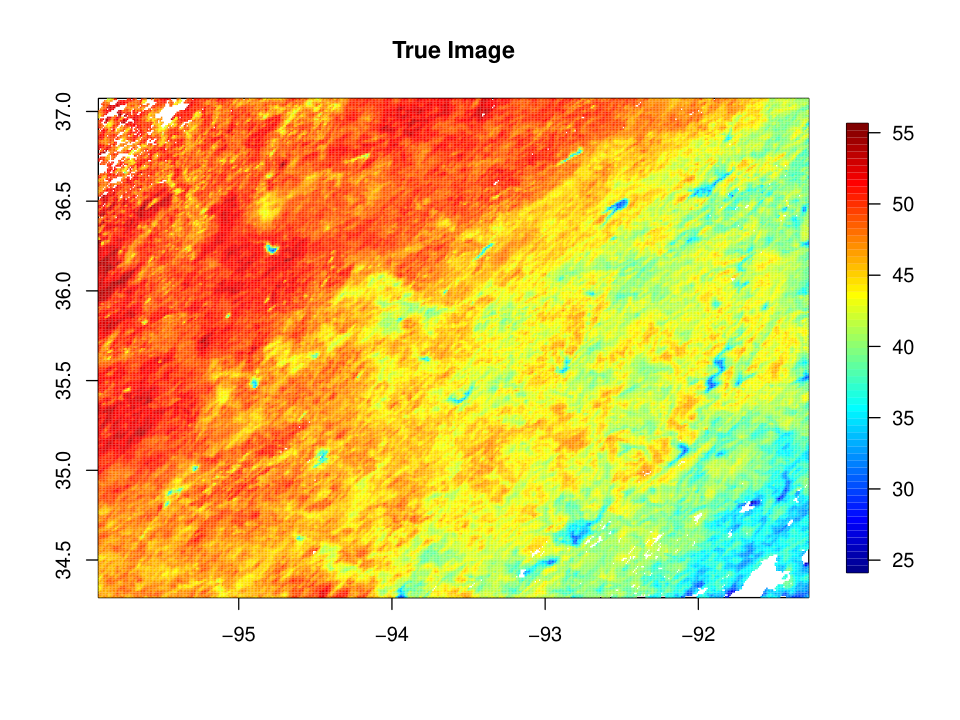


We ran the Kryging algorithm with , , and . For each value of , we use different initial values and pick the best one using five-fold cross-validation within the training dataset. The mean absolute error (MAE), root mean squared error (RMSE), continuously ranked probability score (CRPS), interval score (INT) and pointwise coverage (CVG) for the predictions of the test set datapoints were computed for each case and the computation times were noted and are tabulated in Table 4. Figure 1 shows the estimates (bottom left) and corresponding standard errors (bottom right) for the data. The estimated image picks up all the spatial features in the true data, indicating a good fit. Since the same dataset was also analyzed by twelve other existing methods, the above mentioned metrics for which are available in the Heaton et al. 2019 paper. The relevant results, as presented in the original paper, are presented in Table 5. This allows us a chance to compare the performance of our method to other existing methods, although the computing platforms were not the same for the two cases.
MAE RMSE CRPS INT CVG Run time (min.) Cores used 1.43 1.95 1.07 10.97 0.93 11.18 4 1.43 1.85 1.04 9.74 0.93 15.10 4 1.36 1.78 0.99 9.60 0.93 19.59 4 1.36 1.79 0.99 9.68 0.93 27.01 4
Method MAE RMSE CRPS INT CVG Run time(min) Cores used FRK 1.96 2.44 1.44 14.08 0.70 2.32 1 Gapfill 1.33 1.86 1.17 34.78 0.36 1.39 40 LatticeKrig 1.22 1.68 0.87 7.55 0.96 27.92 1 LAGP 1.65 2.08 1.17 10.81 0.83 2.27 40 Metakriging 2.08 2.50 1.44 10.77 0.89 2888.52 30 MRA 1.33 1.85 0.94 8.00 0.92 15.61 1 NNGP 1.21 1.64 0.85 7.57 0.95 2.06 10 Partition 1.41 1.80 1.02 10.49 0.86 79.98 55 Pred. Proc. 2.15 2.64 1.55 15.51 0.83 160.24 10 SPDE 1.10 1.53 0.83 8.85 0.97 120.33 2 Tapering 1.87 2.45 1.32 10.31 0.93 133.26 1 Periodic Embedding 1.29 1.79 0.91 7.44 0.93 9.81 1
In terms of RMSE and coverage, SPDE (Lindgren et al. 2011), Nearest Neighbor Gaussian Process or NNGP (Datta et al. 2016a; Datta et al. 2016b; Datta et al. 2016c) and LatticeKrig (Nychka et al. 2015) perform better than the proposed method. The time taken by the method is significantly less than the SPDE method and comparable to LatticeKrig. Although it should be mentioned that the they were run in different platforms with similar hardware set-up, so the comparison should not be considered a direct one. The time presented for the NNGP method in Heaton et al. 2019 considers only the time taken for the conjugate model where a well defined grid of possible parameter values were supplied to the model to use cross-validation in parallel. This range of parameter values need to be determined first and is the more difficult and time consuming part of any existing approximate inference method and neither the strategy nor the time taken to arrive at those numbers were reported in Heaton et al. 2019.
6 Conclusion
In this article, we propose an approximate inference method for analyzing massive spatial datasets using Krylov subspace approximation and profile maximum likelihood methods. The method assumes that the underlying process realizations are on a regular equispaced grid, but the observations need not be colocated on the grid. While we exclusively model the spatial process covariance using the Matrn covariance family, the method works for any choice of stationary covariance function. We also propose an approach to approximate log-determinants for symmetric BTTB matrices which has guaranteed asymptotic convergence to the true log-determinant value. The method has computational complexity of , resulting in fast run times and excellent scalability with the sample size while producing decent estimates and requires little tuning. The method is expected to run especially well when the spatial range is small to moderate and partial sill to nugget ratio is moderate. This is seen in the applications involving both synthetic and real datasets.
Although uncertainties for the mean and spatial parameter estimates are not provided directly, they can be obtained using the following approaches. A reasonable approach would be to compute the exact Hessian and its inverse for the optimization process of Eq. (13). However, that is time consuming as it has complexity involved with the computation. A suitable approximation to the inverse of the Hessian will be needed to efficiently estimate the uncertainties associated with these parameters. A computationally-expensive alternative is to estimate the parameters using the parametric bootstrap, as outlined in Section 3.5.
The method is proposed as a -dimensional method. However, for irregular datasets on dimensions higher than 3, the grid formation is slow and difficult. But for the purposes of geostatistical analyses, we need only concern ourselves with problems in or where grids are simple and easy to deal with. Should the case arise where one has to deal with higher dimensional geospatial analysis, one needs to look for a suitable alternative to the grid structure which can be a future avenue for research. Moreover, Kryging is most attractive when the observations are approximately on a grid or uniformly distributed and adaptations for extremely irregular cases such as data observed along transects or in separated clusters is another area of future work.
The proposed model can be utilized in many other scenarios than simply what has been illustrated in this article. The computational amenities of the method can be utilized for spatiotemporal modeling. Changing the observational model to include two or more sources of data can be contemplated as well. Quantifying uncertainties for the mean and the spatial parameters can be one possible extension. Extending the method to non-Gaussian observational models, for example, binary or count data, would be another possibility.
Acknowledgements
The authors were partially supported by the National Science Foundation through the awards DMS-1845406 and DMS-1638521. The authors were also partially supported by the National Institute of Health through the awards
R01ES031651-01 and R01ES027892 and by The King Abdullah University of Science and Technology grant 3800.2. We would like to thank them for their support.
Declarations
Funding
The authors were partially supported by the National Science Foundation through the awards DMS-1845406 and DMS-1638521. The authors were also partially supported by the National Institute of Health through the awards
R01ES031651-01 and R01ES027892 and by The King Abdullah University of Science and Technology grant 3800.2.
Conflict of Interest
The authors have no conflicts of interest to declare that are relevant to the content of this article.
Availability of Data and Material
The dataset analyzed in Section 5 is available in the GitHub repository for the Heaton et al. 2019 project at this GitHub repository.
Code Availability
A GitHub repository has been set up that contains codes and a demonstration file for the methods described in the article.
Ethics Approval
Not Applicable
Consent to Participate
Not Applicable
Consent for Publication
Not Applicable
References
- Ambikasaran et al. (2015) Ambikasaran S, Foreman-Mackey D, Greengard L, Hogg DW, O’Neil M (2015) Fast direct methods for Gaussian processes. IEEE transactions on pattern analysis and machine intelligence 38(2):252–265
- Anitescu et al. (2012) Anitescu M, Chen J, Wang L (2012) A matrix-free approach for solving the parametric Gaussian process maximum likelihood problem. SIAM Journal on Scientific Computing 34(1):A240–A262
- Aune et al. (2014) Aune E, Simpson DP, Eidsvik J (2014) Parameter estimation in high dimensional gaussian distributions. Statistics and Computing 24(2):247–263
- Banerjee et al. (2008) Banerjee S, Gelfand AE, Finley AO, Sang H (2008) Gaussian predictive process models for large spatial data sets. Journal of the Royal Statistical Society: Series B (Statistical Methodology) 70(4):825–848
- Barbian and Assunção (2017) Barbian MH, Assunção RM (2017) Spatial subsemble estimator for large geostatistical data. Spatial Statistics 22:68–88
- Benbow (1999) Benbow SJ (1999) Solving generalized least-squares problems with LSQR. SIAM Journal on Matrix Analysis and Applications 21(1):166–177
- Bradley et al. (2016) Bradley JR, Cressie N, Shi T, et al. (2016) A comparison of spatial predictors when datasets could be very large. Statistics Surveys 10:100–131
- Chung and Saibaba (2017) Chung J, Saibaba AK (2017) Generalized hybrid iterative methods for large-scale Bayesian inverse problems. SIAM Journal on Scientific Computing 39(5):S24–S46
- Chung et al. (2018) Chung J, Saibaba AK, Brown M, Westman E (2018) Efficient generalized Golub–Kahan based methods for dynamic inverse problems. Inverse Problems 34(2):024005
- Cox and Snell (1989) Cox DR, Snell EJ (1989) Analysis of binary data, vol 32. CRC press
- Cressie and Johannesson (2008) Cressie N, Johannesson G (2008) Fixed rank Kriging for very large spatial data sets. Journal of the Royal Statistical Society: Series B (Statistical Methodology) 70(1):209–226
- Datta et al. (2016a) Datta A, Banerjee S, Finley AO, Gelfand AE (2016a) Hierarchical nearest-neighbor Gaussian process models for large geostatistical datasets. Journal of the American Statistical Association 111(514):800–812
- Datta et al. (2016b) Datta A, Banerjee S, Finley AO, Gelfand AE (2016b) On nearest-neighbor Gaussian process models for massive spatial data. Wiley Interdisciplinary Reviews: Computational Statistics 8(5):162–171
- Datta et al. (2016c) Datta A, Banerjee S, Finley AO, Hamm NA, Schaap M (2016c) Nonseparable dynamic nearest neighbor Gaussian process models for large spatio-temporal data with an application to particulate matter analysis. The Annals of Applied Statistics 10(3):1286
- Den Hertog et al. (2006) Den Hertog D, Kleijnen JP, Siem AY (2006) The correct Kriging variance estimated by bootstrapping. Journal of the Operational Research Society 57(4):400–409
- Dutta and Mondal (2016) Dutta S, Mondal D (2016) REML estimation with intrinsic Matérn dependence in the spatial linear mixed model. Electronic Journal of Statistics 10(2):2856–2893
- Eidsvik et al. (2014) Eidsvik J, Shaby BA, Reich BJ, Wheeler M, Niemi J (2014) Estimation and prediction in spatial models with block composite likelihoods. Journal of Computational and Graphical Statistics 23(2):295–315
- Eriksson et al. (2018) Eriksson D, Dong K, Lee E, Bindel D, Wilson AG (2018) Scaling Gaussian process regression with derivatives. In: Advances in Neural Information Processing Systems, pp 6867–6877
- Finley et al. (2009) Finley AO, Sang H, Banerjee S, Gelfand AE (2009) Improving the performance of predictive process modeling for large datasets. Computational Statistics & Data Analysis 53(8):2873–2884
- Fuentes (2007) Fuentes M (2007) Approximate likelihood for large irregularly spaced spatial data. Journal of the American Statistical Association 102(477):321–331
- Furrer et al. (2006) Furrer R, Genton MG, Nychka D (2006) Covariance tapering for interpolation of large spatial datasets. Journal of Computational and Graphical Statistics 15(3):502–523
- Gneiting et al. (2006) Gneiting T, Ševčíková H, Percival DB, Schlather M, Jiang Y (2006) Fast and exact simulation of large Gaussian lattice systems in : Exploring the limits. Journal of Computational and Graphical Statistics 15(3):483–501
- Graham et al. (2018) Graham IG, Kuo FY, Nuyens D, Scheichl R, Sloan IH (2018) Analysis of circulant embedding methods for sampling stationary random fields. SIAM Journal on Numerical Analysis 56(3):1871–1895
- Gray (2006) Gray RM (2006) Toeplitz and circulant matrices: A review. Foundations and Trends® in Communications and Information Theory 2(3):155–239
- Guhaniyogi and Banerjee (2018) Guhaniyogi R, Banerjee S (2018) Meta-Kriging: Scalable Bayesian modeling and inference for massive spatial datasets. Technometrics 60(4):430–444
- Guinness (2019) Guinness J (2019) Spectral density estimation for random fields via periodic embeddings. Biometrika 106(2):267–286
- Guinness and Fuentes (2017) Guinness J, Fuentes M (2017) Circulant embedding of approximate covariances for inference from Gaussian data on large lattices. Journal of Computational and Graphical Statistics 26(1):88–97
- Gyires (1956) Gyires B (1956) Eigenwerte verallgemeinerter Toeplitzschen matrizen. Publ Math Debrecen 4:171–179
- Heaton et al. (2019) Heaton MJ, Datta A, Finley AO, Furrer R, Guinness J, Guhaniyogi R, Gerber F, Gramacy RB, Hammerling D, Katzfuss M, et al. (2019) A case study competition among methods for analyzing large spatial data. Journal of Agricultural, Biological and Environmental Statistics 24(3):398–425
- Higdon (2002) Higdon D (2002) Space and space-time modeling using process convolutions. In: Quantitative methods for current environmental issues, Springer, pp 37–56
- Kang and Cressie (2011) Kang EL, Cressie N (2011) Bayesian inference for the spatial random effects model. Journal of the American Statistical Association 106(495):972–983
- Katzfuss (2017) Katzfuss M (2017) A multi-resolution approximation for massive spatial datasets. Journal of the American Statistical Association 112(517):201–214
- Katzfuss and Cressie (2011) Katzfuss M, Cressie N (2011) Spatio-temporal smoothing and EM estimation for massive remote-sensing data sets. Journal of Time Series Analysis 32(4):430–446
- Katzfuss and Hammerling (2017) Katzfuss M, Hammerling D (2017) Parallel inference for massive distributed spatial data using low-rank models. Statistics and Computing 27(2):363–375
- Kaufman et al. (2008) Kaufman CG, Schervish MJ, Nychka DW (2008) Covariance tapering for likelihood-based estimation in large spatial data sets. Journal of the American Statistical Association 103(484):1545–1555
- Kent and Mardia (1996) Kent JT, Mardia KV (1996) Spectral and circulant approximations to the likelihood for stationary Gaussian random fields. Journal of statistical planning and inference 50(3):379–394
- Lindgren et al. (2011) Lindgren F, Rue H, Lindström J (2011) An explicit link between Gaussian fields and Gaussian Markov random fields: the stochastic partial differential equation approach. Journal of the Royal Statistical Society: Series B (Statistical Methodology) 73(4):423–498
- Liu et al. (2020) Liu H, Ong YS, Shen X, Cai J (2020) When Gaussian process meets big data: A review of scalable GPs. IEEE Transactions on Neural Networks and Learning Systems
- Martino and Rue (2009) Martino S, Rue H (2009) Implementing approximate bayesian inference using integrated nested laplace approximation: A manual for the inla program. Department of Mathematical Sciences, NTNU, Norway
- Matérn (1960) Matérn B (1960) Spatial variation, volume 36 of. Lecture Notes in Statistics
- Minden et al. (2017) Minden V, Damle A, Ho KL, Ying L (2017) Fast spatial Gaussian process maximum likelihood estimation via skeletonization factorizations. Multiscale Modeling & Simulation 15(4):1584–1611
- Nychka et al. (2015) Nychka D, Bandyopadhyay S, Hammerling D, Lindgren F, Sain S (2015) A multiresolution Gaussian process model for the analysis of large spatial datasets. Journal of Computational and Graphical Statistics 24(2):579–599
- Paciorek et al. (2015) Paciorek CJ, Lipshitz B, Zhuo W, Kaufman CG, Thomas RC, et al. (2015) Parallelizing Gaussian Process Calculations in R. Journal of Statistical Software 63(i10)
- Rue and Held (2005) Rue H, Held L (2005) Gaussian Markov random fields: theory and applications. CRC press
- Saad (2003) Saad Y (2003) Iterative methods for sparse linear systems, 2nd edn. Society for Industrial and Applied Mathematics, Philadelphia, PA, DOI 10.1137/1.9780898718003, URL https://doi-org.prox.lib.ncsu.edu/10.1137/1.9780898718003
- Stein (2002) Stein ML (2002) Fast and exact simulation of fractional Brownian surfaces. Journal of Computational and Graphical Statistics 11(3):587–599
- Stein (2013) Stein ML (2013) Statistical properties of covariance tapers. Journal of Computational and Graphical Statistics 22(4):866–885
- Stein et al. (2004) Stein ML, Chi Z, Welty LJ (2004) Approximating likelihoods for large spatial data sets. Journal of the Royal Statistical Society: Series B (Statistical Methodology) 66(2):275–296
- Sun et al. (2012) Sun Y, Li B, Genton MG (2012) Geostatistics for large datasets. In: Advances and challenges in space-time modelling of natural events, Springer, pp 55–77
- Ubaru et al. (2017) Ubaru S, Chen J, Saad Y (2017) Fast estimation of tr(f()) via stochastic Lanczos quadrature. SIAM Journal on Matrix Analysis and Applications 38(4):1075–1099
- Varin et al. (2011) Varin C, Reid N, Firth D (2011) An overview of composite likelihood methods. Statistica Sinica pp 5–42
- Vecchia (1988) Vecchia AV (1988) Estimation and model identification for continuous spatial processes. Journal of the Royal Statistical Society: Series B (Methodological) 50(2):297–312
- Wendland (1995) Wendland H (1995) Piecewise polynomial, positive definite and compactly supported radial functions of minimal degree. Advances in Computational Mathematics 4(1):389–396
- Widom (1974) Widom H (1974) Asymptotic behavior of block Toeplitz matrices and determinants. Advances in Mathematics 13(3):284–322
APPENDIX
Appendix A Gradient and Hessian Computation for the Optimization Procedure
In this section, we present the necessary details of computing and approximating the gradient and Hessian for the optimization routine.
We first, derive exact expressions for the gradient and then show how to approximate them using the strategy in Sections 3.2 and 3.1. Computing the analytical gradient would require computing derivatives of and with respect to each of and . For convenience, we reparametrize and . Using the precision instead of variance brings about greater ease in computing the analytical derivatives. Under the new parametrization,
| (15) |
| (16) |
and
| (17) |
where .
The derivatives for are computed to be
| (18) |
where denotes the derivative of with respect to . This is easy to compute analytically and has the nice BTTB property that has.
Using the expressions in (18), we compute the derivatives of to be
| (19) |
Substituting the expressions for analytical derivatives of and in the expression for the analytical gradient, we have it computed to be
| (20) |
where dL is the derivative of with respect to .
We approximate the gradient expressions in (20) by approximating by as in (12) and using the exact arithmetic identities expressed in (10). The approximated gradients can be computed as
| (21) |
where and have been defined in Section 3.2.
is an approximation to dL, the derivative of the log-determinant of with respect to . The analytical expression for dL turns out to be
This is infeasible to compute directly and is therefore approximated using the BTTB structure of and .
Any symmetric matrix with BTTB structure can be extended to have a BCCB structure as was done in computing the log-determinant itself and one can extract the eigenvalues of the matrix with BTTB structure using the matrix with BCCB structure. Any BCCB matrix is diagonalizable as , where is a scaled matrix consisting of -dimensional (d=2, in our case) Fourier coefficients, irrespective of the BCCB matrix being diagonalized. Therefore, we can say
| (22) |
These imply that
| (23) |
Since both and are diagonal, approximating dL boils down to computing and which can be computed by -dimensional FFT of the corresponding first circulant block structures of the extended BCCB structure and subsetting it properly. The equivalence in computing the derivative of log-determinant of the BTTB and matrix and its corresponding BCCB matrix has been demonstrated by Kent and Mardia 1996, showing the approximation to have the same error rate as in approximating the log-determinant itself. Approximating the derivative of the log-determinant term also costs the same as approximating the log-determinant itself, .
While minimizing the negative log-likelihood function, the Hessian turns out to be simply the Information matrix . While
we also have
Here the expectations are computed with respect to and , represent the gradient and Hessian created by computing first and second order partial derivatives with respect to . Therefore, the outer product of the gradient with itself serves as a rank-one estimate for the Hessian for a likelihood optimization problem. Although we are using profile likelihood instead of the actual likelihood function, the approximation still stands in an asymptotic sense since both the actual likelihood estimator and the profile likelihood estimators have the same asymptotic properties. This prompts us to take the outer product of the approximated gradient with itself as a rank-one approximation to the Hessian.
However, we compute the unique entries of the exact Hessian to be
| (24) |
where represents the second derivative of with respect to and is the second derivative of with respect to . also has a BTTB structure as and .
These entries are then approximated using the approximation to as presented in Chung et al. 2018, namely
| (25) |
where with and .
We define . The approximated entries of the Hessian are
| (26) |
where is a numerical approximation to . We do not use this approximation for our computing, but hope to use it in future.
Appendix B Additional Tables from the Simulation Study
In this section, we provide additional results for the simulation study. Table 6 evaluates parameter estimations for the first simulation study for both SPDE and Kryging methods. The same is done in Tables 7 and 8 for the second and third simulation studies. The results across the board are similar as mentioned in Section 4. SPDE performs better in estimating the nugget parameter , while Kryging performs better in estimating the partial sill parameter . Both methods do equally well in estimating the mean parameter and the spatial range parameter .
Parameter Grid Size SPDE Kryging k=20 k=50 k=100 k=200 0.30 (0.30) 0.31 (0.32) 0.30 (0.32) 0.31 (0.32) 0.31 (0.32) 0.23 (0.22) 0.28 (0.23) 0.28 (0.23) 0.28 (0.23) 0.28 (0.23) 0.32 (0.24) 0.32 (0.25) 0.32 (0.25) 0.32 (0.25) 0.32 (0.25) 0.26 (0.26) 0.29 (0.26) 0.29 (0.26) 0.29 (0.26) 0.29 (0.26) 1.43 (0.11) 0.36 (0.34) 0.36 (0.34) 0.36 (0.34) 0.36 (0.34) 1.59 (0.07) 0.31 (0.24) 0.31 (0.24) 0.31 (0.24) 0.31 (0.24) 1.70 (0.07) 0.33 (0.26) 0.33 (0.26) 0.33 (0.26) 0.33 (0.26) 1.81 (0.06) 0.30 (0.17) 0.30 (0.17) 0.30 (0.17) 0.30 (0.17) 0.10 (0.01) 0.17 (0.05) 0.17 (0.05) 0.17 (0.05) 0.17 (0.05) 0.06 (0.01) 0.16 (0.04) 0.16 (0.04) 0.16 (0.04) 0.16 (0.04) 0.05 (0.00) 0.16 (0.05) 0.16 (0.05) 0.16 (0.05) 0.16 (0.05) 0.04 (0.00) 0.19 (0.03) 0.19 (0.03) 0.19 (0.03) 0.19 (0.03) 0.06 (0.02) 0.03 (0.00) 0.03 (0.00) 0.02 (0.00) 0.02 (0.00) 0.01 (0.01) 0.03 (0.00) 0.03 (0.00) 0.03 (0.00) 0.03 (0.00) 0.01 (0.01) 0.03 (0.00) 0.03 (0.00) 0.03 (0.00) 0.03 (0.00) 0.03 (0.00) 0.03 (0.00) 0.03 (0.00) 0.03 (0.00) 0.03 (0.00)
Parameter Setting SPDE Kryging k=20 k=50 k=100 k=200 Setting 1 0.16 (0.15) 0.16 (0.14) 0.16 (0.14) 0.16 (0.14) 0.16 (0.14) Setting 2 0.42 (0.37) 0.46 (0.39) 0.46 (0.39) 0.46 (0.39) 0.46 (0.39) Setting 3 0.18 (0.10) 0.22 (0.10) 0.22 (0.10) 0.22 (0.10) 0.22 (0.10) Setting 4 0.42 (0.27) 0.43 (0.28) 0.43 (0.28) 0.43 (0.28) 0.43 (0.28) Setting 1 1.43 (0.05) 0.16 (0.17) 0.16 (0.17) 0.16 (0.17) 0.16 (0.17) Setting 2 1.79 (0.11) 0.59 (0.32) 0.59 (0.32) 0.59 (0.32) 0.59 (0.32) Setting 3 0.47 (0.06) 0.23 (0.21) 0.23 (0.21) 0.23 (0.21) 0.23 (0.21) Setting 4 4.07 (0.06) 0.70 (0.44) 0.70 (0.44) 0.70 (0.44) 0.70 (0.44) Setting 1 0.10 (0.01) 0.16 (0.02) 0.16 (0.02) 0.16 (0.02) 0.16 (0.02) Setting 2 0.04 (0.01) 0.21 (0.06) 0.21 (0.06) 0.21 (0.06) 0.21 (0.06) Setting 3 0.07 (0.15) 0.30 (0.03) 0.30 (0.03) 0.30 (0.03) 0.30 (0.03) Setting 4 0.12 (0.01) 0.10 (0.06) 0.10 (0.06) 0.10 (0.06) 0.10 (0.06) Setting 1 0.03 (0.00) 0.02 (0.00) 0.02 (0.00) 0.02 (0.00) 0.02 (0.00) Setting 2 0.05 (0.02) 0.13 (0.00) 0.13 (0.00) 0.13 (0.00) 0.13 (0.00) Setting 3 0.03 (0.02) 0.03 (0.00) 0.03 (0.00) 0.03 (0.00) 0.03 (0.00) Setting 4 0.01 (0.00) 0.03 (0.00) 0.03 (0.00) 0.03 (0.00) 0.03 (0.00)
Parameter Gridsize SPDE Kryging k=20 k=50 k=100 0.24 (0.18) 0.29 (0.16) 0.29 (0.16) 0.29 (0.16) 0.24 (0.18) 0.29 (0.16) 0.29 (0.16) 0.29 (0.16) 0.24 (0.18) 0.29 (0.16) 0.29 (0.16) 0.29 (0.16) 1.61 (0.07) 0.26 (0.21) 0.26 (0.21) 0.26 (0.21) 1.61 (0.07) 0.26 (0.21) 0.26 (0.21) 0.26 (0.21) 1.61 (0.07) 0.26 (0.21) 0.26 (0.21) 0.26 (0.21) 0.06 (0.01) 0.17 (0.04) 0.17 (0.04) 0.17 (0.04) 0.06 (0.01) 0.17 (0.04) 0.17 (0.04) 0.17 (0.04) 0.06 (0.01) 0.17 (0.04) 0.17 (0.04) 0.17 (0.04) 0.01 (0.01) 0.03 (0.00) 0.03 (0.00) 0.03 (0.00) 0.01 (0.01) 0.03 (0.00) 0.03 (0.00) 0.03 (0.00) 0.01 (0.01) 0.03 (0.00) 0.03 (0.00) 0.03 (0.00)