跳到论文正文
W Papers独立论文阅读器 arXiv:2012.13115 论文正文 计算阅读时间 · 0%
引用这篇论文根据当前论文元数据生成,正式投稿前建议核对。


License: arXiv.org perpetual non-exclusive license
arXiv:2012.13115v1 [cs.LG] 24 Dec 2020

Upper Confidence Bounds for Combining Stochastic Bandits

Ashok Cutkosky Affiliation: Boston University Affiliation: Boston, MA Email: ashok@cutkosky.com    Abhimanyu Das Affiliation: Google Research Affiliation: Mountain View, CA Email: abhidas@google.com    Manish Purohit Affiliation: Google Research Affiliation: Mountain View, CA Email: mpurohit@google.com
Abstract

We provide a simple method to combine stochastic bandit algorithms. Our approach is based on a “meta-UCB” procedure that treats each of NN individual bandit algorithms as arms in a higher-level NN-armed bandit problem that we solve with a variant of the classic UCB algorithm. Our final regret depends only on the regret of the base algorithm with the best regret in hindsight. This approach provides an easy and intuitive alternative strategy to the CORRAL algorithm for adversarial bandits, without requiring the stability conditions imposed by CORRAL on the base algorithms. Our results match lower bounds in several settings, and we provide empirical validation of our algorithm on misspecified linear bandit and model selection problems.

1 Introduction

This paper studies the classic contextual bandit problem in a stochastic setting [1, 2], which is a generalization of the even more classical multi-armed bandit problem [3]. In each of TT rounds indexed by t=1,…,Tt=1,\dots,T, we observe an i.i.d. random context ct∈Cc_{t}\in C, which we use to select an action at=xt​(ct)∈Aa_{t}=x_{t}(c_{t})\in A based on some policy xt:C→Ax_{t}:C\to A. Then, we receive a noisy reward r^t∈[0,1]\hat{r}_{t}\in[0,1], whose expectation is a function of only ctc_{t} and ata_{t}: 𝔼[rt|ct,at]=r(ct,at)\mathop{\mathbb{E}}[r_{t}|c_{t},a_{t}]=r(c_{t},a_{t}). The goal is to perform nearly as well as the best policy in hindsight by minimizing the regret:

Regret=∑t=1Tr⋆−r⁡(ct,at)\displaystyle\text{Regret}=\sum_{t=1}^{T}r_{\star}-r(c_{t},a_{t})

where r⋆=infx∈X𝔼c[r⁡(c,x⁡(c))]r_{\star}=\inf_{x\in X}\mathop{\mathbb{E}}_{c}[r(c,x(c))], and XX is some space of possible policies.

This problem and variants has been extensively studied under diverse assumptions about the space of policies XX and distributions of the rewards and values for r⋆r_{\star}. (e.g. see [4, 1, 2, 5, 6, 7]). Many of these algorithms have different behaviors in different environments (e.g. one algorithm might do much better if the reward r⁡(ct,at)r(c_{t},a_{t}) is a linear function of the context, while another might do better if the reward is independent of the context). This plethora of prior algorithms necessitates a “meta-decision”: If the environment is not known in advance, which algorithm should be used for the task at hand? Even in hindsight, it may not be obvious which algorithm was most optimized for the experienced environment, and so this meta-decision can be quite difficult.

We model this meta-decision by assuming we have access to NN base bandit algorithms 𝒜1,…,𝒜N\mathcal{A}_{1},\dots,\mathcal{A}_{N}. We will attempt to design a meta-algorithm whose regret is comparable to the best regret experienced by any base algorithm in hindsight for the current environment. Since we don’t know in advance which base algorithm will be optimal for the current environment, we need to address this problem in an online fashion. On the ttth round, we will choose some index iti_{t} and play the action suggested by the algorithm 𝒜it\mathcal{A}_{i_{t}}. The primary difficulty is that some base algorithms might perform poorly at first, and then begin to perform well later. A naive strategy might discard such algorithms based on the poor early performance, so some enhanced form of exploration is necessary for success. A pioneering prior work on this setting has considered the adversarial rather than stochastic case [8], and utilizes a sampling based on mirror descent with a clever mirror-map. Somewhat simplifying these results, suppose each algorithm 𝒜i\mathcal{A}_{i} guarantees regret Ci​TαiC_{i}T^{\alpha_{i}} for some CiC_{i} and αi\alpha_{i}11 1 in many common settings, αi=1/2\alpha_{i}=1/2. Given a user-specified learning rate parameter η∈ℝ\eta\in\mathbb{R}, [8, 9] guarantee:

Regret≤minj≤N⁡Cj1αj​T​η1−αjαj+T​η+Nη\displaystyle\text{Regret}\leq\min_{j\leq N}C_{j}^{\frac{1}{\alpha_{j}}}T\eta^{\frac{1-\alpha_{j}}{\alpha_{j}}}+T\eta+\frac{N}{\eta} (1)

The value of η\eta is chosen apriori, but the values of CiC_{i} need not be known. To gain a little intuition for this expression, suppose all αi=1/2\alpha_{i}=1/2, and set η=NT\eta=\frac{\sqrt{N}}{\sqrt{T}}. Then the regret is mini≤N⁡Ci2​N​T\min_{i\leq N}C_{i}^{2}\sqrt{NT}.

In this paper, we leverage the stochastic environment to avoid requiring some technical stability conditions needed in [8]: our result is a true black-box meta-algorithm that does not require any modifications to the base algorithms. Moreover, our general technique is in our view both different and much simpler. Our regret bound also improves on (1) by virtue of being non-uniform over the base algorithms: given any parameters η1,…,ηN\eta_{1},\dots,\eta_{N}, we obtain

Regret≤minj≤N⁡Cj1αj​T​ηj1−αjαj+T​ηj+∑i≠j1ηi\displaystyle\text{Regret}\leq\min_{j\leq N}C_{j}^{\frac{1}{\alpha_{j}}}T\eta_{j}^{\frac{1-\alpha_{j}}{\alpha_{j}}}+T\eta_{j}+\sum_{i\neq j}\frac{1}{\eta_{i}} (2)

This recovers (1) when all ηi\eta_{i} are equal. In general one can think of the values 1ηi\frac{1}{\eta_{i}} as specifying a kind of prior over the 𝒜i\mathcal{A}_{i} which allows us to develop more delicate trade-offs between their performances. For example, consider again the setting when all αi=1/2\alpha_{i}=1/2. If we believe that 𝒜1\mathcal{A}_{1} is more likely to perform well, then by setting η1=1T\eta_{1}=\frac{1}{\sqrt{T}} and ηj=NT\eta_{j}=\frac{N}{\sqrt{T}} for j≠1j\neq 1, we can obtain a regret of OPENmin⁡(C12​T,min2≤j≤N⁡Cj2​N​T))\min(C_{1}^{2}\sqrt{T},\min_{2\leq j\leq N}C_{j}^{2}N\sqrt{T})).

This type of bound is in some sense a continuation of a general trend in the bandit community towards finding algorithms that adapt to various properties of the environment that are unknown in foresight (e.g [10, 11, 12, 13]). However, instead of committing to some property (e.g. large value of r⋆r_{\star}, or small variance of r^\hat{r}), we instead design an algorithm that is in some sense “future-proof”, as new algorithms can be easily incorporated as new base algorithms 𝒜i\mathcal{A}_{i}.

In a recent independent work, [9] has extended the techniques of [8] to our same stochastic setting. They use a clever smoothing technique to also dispense with the stability condition required by [8], and achieve the regret bound (1). In addition to achieving the non-uniform bound (2), we also improve upon their work in two other ways: our algorithm requires only O⁡(N)O(N) space in contrast to O⁡(T​N)O(TN) space, and we allow for our base algorithms to only guarantee in-expectation rather than high-probability bounds.

In the stochastic setting, it is frequently possible to obtain logarithmic regret subject to various forms of “gap” assumptions on the actions. However, the method of [8], even when considered in the stochastic setting as in [9], seems unable to obtain such bounds. Instead, [14] has recently provided a method based on UCB that can achieve such results. Their algorithm is similar to ours, but we devise a somewhat more intricate method that is able to not only obtain the results outlined previously, but also match the logarithmic regret bounds provided by [14].

In the stochastic setting, [15] introduces a new model selection technique called Regret Balancing. However this approach requires knowledge of the exact regret bounds of the optimal base algorithm. Our approach not only avoids this requirement, but also results in stronger regret guarantees than those in that paper.

We also consider an extension of our techniques to the setting of linear contextual bandits with adversarial features. In this case we require some modifications to our combiner algorithm and assume that the base algorithms are in fact instances of linUCB [16] or similar confidence-ellipsoid based algorithms. However, subject to these restrictions we are able to recover essentially similar results as in the non-adversarial setting, which we present in Section G.

The rest of this paper is organized as follows. In section 2 we describe our formal setup and some assumptions. In section 3 we provide our algorithm and main regret bound in a high-probability setting. In section 5, we extend our analysis to in-expectation regret bounds as well as providing an automatic tuning of some parameters in the main algorithm. In section 6 we sketch some ways in which our algorithm can be applied, and show that it matches some prior lower bound frontiers. Finally, in section 7 we provide empirical validation of our algorithm.

2 Problem Setup

We let AA be a space of actions, XX a space of policies, and CC a space of contexts. Each policy is a function C→AC\to A. (random policies can be modeled by pushing the random bits into the context). In each round t=1,…,Tt=1,\dots,T we choose xt∈Xx_{t}\in X, then see an i.i.d. random context ctc_{t}, and then receive a random reward r^t∈[0,1]\hat{r}_{t}\in[0,1]. Let HtH_{t} denote the sequence x1,c1,r^1,…,r^t−1,xt,ctx_{1},c_{1},\hat{r}_{1},\dots,\hat{r}_{t-1},x_{t},c_{t}. There is an unknown function r:C×A→ℝr:C\times A\to\mathbb{R} such that 𝔼[r^t|Ht]=r⁡(ct,xt​(ct))\mathop{\mathbb{E}}[\hat{r}_{t}|H_{t}]=r(c_{t},x_{t}(c_{t})) for any HtH_{t}. The distribution of r^t\hat{r}_{t} is independent of all other values conditioned on xtx_{t} and ctc_{t}. We will also write r⁡(x)=𝔼c∼𝒟c[r⁡(c,x)]r(x)=\mathop{\mathbb{E}}_{c\sim\mathcal{D}_{c}}[r(c,x)] and rt=r⁡(ct,xt​(ct))r_{t}=r(c_{t},x_{t}(c_{t})). Let x⋆∈argmax⁡r⁡(x)x_{\star}\in\mathop{\text{argmax}}r(x). Define r⋆=𝔼cr⁡(c,x⋆​(c))r_{\star}=\mathop{\mathbb{E}}_{c}r(c,x_{\star}(c)). Then we define the regret (often called “pseudo-regret” instead) as:

Regret=∑t=1Tr⋆−rt\displaystyle\text{Regret}=\sum_{t=1}^{T}r_{\star}-r_{t}

Each base bandit algorithm 𝒜i\mathcal{A}_{i} can be viewed as a randomized procedure that takes any sequence x1,c1,r^1,…,xt−1,ct−1,r^t−1x_{1},c_{1},\hat{r}_{1},\dots,x_{t-1},c_{t-1},\hat{r}_{t-1} and outputs some xt∈Xx_{t}\in X. At the ttth round of the bandit game, our algorithm will choose some index it∈{1,…,N}i_{t}\in\{1,\dots,N\}. Then we obtain policy xT⁡(it,t)itx^{i_{t}}_{T(i_{t},t)} from AitA_{i_{t}}, and take action xt=xT⁡(it,t)it​(ct)x_{t}=x^{i_{t}}_{T(i_{t},t)}(c_{t}). The policy xT⁡(it,t)itx^{i_{t}}_{T(i_{t},t)} is the output of AitA_{i_{t}} on the input sequence of policies, contexts, and rewards for all the prior rounds for which we have chosen this same index iti_{t}. After receiving the reward r^t\hat{r}_{t}, we send this reward as feedback to 𝒜it\mathcal{A}_{i_{t}}.

In order to formalize this analysis more cleanly, for all ii, we define TT independent random variables c1i,…,cTic^{i}_{1},\dots,c^{i}_{T}, where each cti∼𝒟cc^{i}_{t}\sim\mathcal{D}_{c}. Further, we define random variables x1i,…,xTix^{i}_{1},\dots,x^{i}_{T} and r^1i,…,r^Ti\hat{r}^{i}_{1},\dots,\hat{r}^{i}_{T} such that xtix^{i}_{t} is the output of 𝒜i\mathcal{A}_{i} on the input sequence x1i,c1i,r^1i,…,xt−1i,ct−1i,r^t−1ix^{i}_{1},c^{i}_{1},\hat{r}^{i}_{1},\dots,x^{i}_{t-1},c^{i}_{t-1},\hat{r}^{i}_{t-1} and r^ti\hat{r}^{i}_{t} is a reward obtained by choosing policy xtix^{i}_{t} with context ctic^{i}_{t}. We also define random variables rti=𝔼[r^ti|x1i,c1i,r^1i,…,r^t−1i,ct−1i]r^{i}_{t}=\mathop{\mathbb{E}}[\hat{r}^{i}_{t}|x^{i}_{1},c^{i}_{1},\hat{r}^{i}_{1},\dots,\hat{r}^{i}_{t-1},c^{i}_{t-1}].

Then we can rephrase the high-level action of our algorithm as follows: We choose some index it∈{1,…,N}i_{t}\in\{1,\dots,N\}. Then we play policy xt=xT⁡(it,t)itx_{t}=x^{i_{t}}_{T(i_{t},t)}, see context ct=cT⁡(it,t)itc_{t}=c^{i_{t}}_{T(i_{t},t)}, and obtain reward r^t=r^T⁡(it,t)it\hat{r}_{t}=\hat{r}^{i_{t}}_{T(i_{t},t)}. We define rt=rT⁡(it,t)itr_{t}=r^{i_{t}}_{T(i_{t},t)}. Note that the distribution of the observed reward ∑t=1Tr^t\sum_{t=1}^{T}\hat{r}_{t} as well as the expected reward ∑t=1Trt\sum_{t=1}^{T}r_{t} is maintained by this description of the random variables.

2.1 Assumptions

We will consider two settings for the base algorithms in our analysis. First, a high-probability setting in which we wish to provide a regret bound that holds with probability at least 1−δ1-\delta for some given δ\delta. Second, an in-expectation setting in which we simply wish to bound the expected value of the regret. In the first setting, we require high-probability bounds on the regret of the base algorithms, while in the second setting we do not. Our approach to the in-expectation setting will be a construction that uses our high-probability algorithm as a black-box. Thus, the majority of our analysis takes place in the high-probability setting (in Section 3), for which we now describe the assumptions.

In the high-probability setting, we assume there are (known) numbers C1,…,CNC_{1},\dots,C_{N} and α1,…,αN∈[12,1]\alpha_{1},\dots,\alpha_{N}\in[\frac{1}{2},1], a δ>0\delta>0 and an (unknown) set S⊂{1,…,N}S\subset\{1,\dots,N\} such that with probability at least 1−δ1-\delta, there is some J∈SJ\in S such that for all t≤Tt\leq T,

∑τ=1tr⋆−rτJ≤CJ​tαJ\displaystyle\sum_{\tau=1}^{t}r_{\star}-r^{J}_{\tau}\leq C_{J}t^{\alpha_{J}} (3)

Intuitively, this is saying that each algorithm 𝒜i\mathcal{A}_{i} comes with a putative regret bound Ci​tαiC_{i}t^{\alpha_{i}}, and with high probability there is some 𝒜i\mathcal{A}_{i} with i∈Si\in S for which its claimed regret bound is in fact correct. The assumption is stronger as SS becomes smaller, and our final results will depend on the size of SS. In Section F, we provide some examples of algorithms that satisfy the requirement (3). Generally, it turns out that most algorithms based the optimism principle can be made to work in this setting for any desired δ\delta. We will refer to an index JJ that satisfied (3) as being “well-specified”.

To gain intuition about our results, we recommend that the reader supposes that SS is a singleton S={J}S=\{J\} for some unknown index JJ, and αi=1/2\alpha_{i}=1/2 for all ii (note that SS may be much smaller than the set of indices for which 3 holds). As a concrete example, suppose |X|=K|X|=K and ct=0c_{t}=0 for all tt, so that we are playing a classic KK-armed bandits problem. Let 𝒜1\mathcal{A}_{1} be an instance of UCB, but restricted to the first 1010 arms, while 𝒜2\mathcal{A}_{2} is instance of UCB restricted to the last K−10K-10 arms. Then, we can set C1=O⁡(10​log⁡(T2/δ)CLOSEC_{1}=O(\sqrt{10\log(T^{2}/\delta)} and C2=O⁡((K−10)​log⁡(T2/δ)CLOSEC_{2}=O(\sqrt{(K-10)\log(T^{2}/\delta)}. Now, depending on which is the optimal arm, we may have S={1}S=\{1\} or S={2}S=\{2\}. Although S={1,2}S=\{1,2\} would also satisfy the assumptions, since our results improve when SS is smaller and SS is unknown to the algorithm, we are free to choose the smallest possible SS.

These assumptions may seem stronger than prior work at first glance: not only do we require high-probability rather than in-expectation regret bounds, we require at least one base algorithm to be well-specified, and we require knowledge of the putative regret bounds through the coefficients CiC_{i} and αi\alpha_{i}. Prior work in this setting (e.g. [8, 9]) dispenses with the last two requirements, and [8] also dispenses with the high-probability requirement. However, it turns out that through a simple doubling construction, we can easily incorporate base algorithms with unknown regret bounds that hold only in expectation into our framework. The ability to handle unknown regret bounds dispenses with the well-specified assumption. We describe this construction and the relevant assumptions in Section 5, and show that it only weakens our analysis by log factors.

3 UCB over Bandits

In this Section, we describe our meta-learner for the high-probability setting. The intuition is based on upper-confidence bounds: first, we observe that the unknown well-specified algorithm 𝒜J\mathcal{A}_{J}’s rewards r^τJ\hat{r}^{J}_{\tau} behave very similarly to independent bounded random variables with mean r⋆r_{\star} in that their average value μ^tJ=1t​∑τ=1tr^τJ\hat{\mu}^{J}_{t}=\frac{1}{t}\sum_{\tau=1}^{t}\hat{r}^{J}_{\tau} concentrates about r⋆r_{\star} with radius CJ​tαJ−1C_{J}t^{\alpha_{J}-1}. From this, one might imagine that for any index ii, the value of μ^ti+Ci​tαi−1\hat{\mu}^{i}_{t}+C_{i}t^{\alpha_{i}-1} gives some kind of upper-confidence bound for the final total reward of algorithm ii. We could then feed these estimates into a UCB-style algorithm that views the NN base algorithms as NN arms. Unfortunately, such an approach is complicated by two issues. First, the putative regret bounds for each 𝒜i\mathcal{A}_{i} may not actually hold, which could damage the validity of our confidence estimates. Second, the confidence bounds for different algorithms may have very imbalanced behavior due to the different values of CiC_{i} and αi\alpha_{i}, and we would like our final regret bound to depend only on CJC_{J} and αJ\alpha_{J}.

We address the first issue by keeping track of the statistic ∑τ=1tμ^τi−r^τi\sum_{\tau=1}^{t}\hat{\mu}^{i}_{\tau}-\hat{r}^{i}_{\tau}. If ∑τ=1tμ^τi−r^τi≥Ci​tαi\sum_{\tau=1}^{t}\hat{\mu}^{i}_{\tau}-\hat{r}^{i}_{\tau}\geq C_{i}t^{\alpha_{i}} at any time, then we can conclude that ii is not the well-specified index JJ and so we simply discard 𝒜i\mathcal{A}_{i}. Moreover, it turns out that so long as ∑τ=1tμ^τi−r^τi≤Ci​tαi\sum_{\tau=1}^{t}\hat{\mu}^{i}_{\tau}-\hat{r}^{i}_{\tau}\leq C_{i}t^{\alpha_{i}}, the rewards r^τi\hat{r}^{i}_{\tau} are “well-behaved” enough that our meta-UCB algorithm can operate correctly.

We address the second issue by employing shifted confidence intervals in a construction analogous to that employed by [17], who designed a KK-armed bandit algorithm with a regret bound that depends on the identity of the best arm. Essentially, each algorithm 𝒜i\mathcal{A}_{i} is associated with a target regret bound, RiR_{i}, and each confidence interval is decreased by RiT\frac{R_{i}}{T}. Assuming RiR_{i} satisfies some technical conditions, this will guarantee that the regret is at most O⁡(RJ)O(R_{J}) for any JJ such that 𝒜J\mathcal{A}_{J} is well-specified.

Formally, our algorithm is provided in Algorithm 1, and its analysis is given in Theorem 1, proved in Appendix B. Note that little effort has been taken to improve the constants or log factors.

Algorithm 1 Bandit Combiner
 Input: Bandit algorithms 𝒜1,…,𝒜N\mathcal{A}_{1},\dots,\mathcal{A}_{N}, numbers C1,…,CNC_{1},\dots,C_{N}, α1,…,αN\alpha_{1},\dots,\alpha_{N}, R1,…,RNR_{1},\dots,R_{N}, TT.
 Set T⁡(i,0)=0T(i,0)=0 for all ii, set μ^0i=0\hat{\mu}^{i}_{0}=0 for all ii, and set I1={1,…,N}I_{1}=\{1,\dots,N\}
 for t=1​…​Tt=1\dots T do
  Set U⁡(i,t−1)=μ^T⁡(i,t−1)i+min⁡(1,Ci​T​(i,t−1)αi+8​log⁡(T3​N/δ)​T​(i,t−1)T⁡(i,t−1))−RiTU(i,t-1)=\hat{\mu}^{i}_{T(i,t-1)}+\min\left(1,\frac{C_{i}T(i,t-1)^{\alpha_{i}}+\sqrt{8\log(T^{3}N/\delta)T(i,t-1)}}{T(i,t-1)}\right)-\frac{R_{i}}{T} for all ii.
  Set it=argmaxi∈It⁡U⁡(i,t−1)i_{t}=\mathop{\text{argmax}}_{i\in I_{t}}U(i,t-1).
  Update T⁡(it,t)=T⁡(it,t−1)+1T(i_{t},t)=T(i_{t},t-1)+1 and T⁡(j,t)=T⁡(j,t−1)T(j,t)=T(j,t-1) for j≠itj\neq i_{t}.
  Get T⁡(it,t)T(i_{t},t)th policy xt=xT⁡(it,t)itx_{t}=x^{i_{t}}_{T(i_{t},t)} from AitA_{i_{t}}. See context ctc_{t} and play action xt​(ct)x_{t}(c_{t}).
  Receive reward r^t=r^T⁡(it,t)i\hat{r}_{t}=\hat{r}^{i}_{T(i_{t},t)}, provide reward r^t\hat{r}_{t} and context ctc_{t} as feedback to 𝒜it\mathcal{A}_{i_{t}}.
  Update μ^T⁡(it,t)it=1T⁡(it,t)​∑τ=1T⁡(it,t)r^τit\hat{\mu}^{i_{t}}_{T(i_{t},t)}=\frac{1}{T(i_{t},t)}\sum_{\tau=1}^{T(i_{t},t)}\hat{r}^{i_{t}}_{\tau}.
  if ∑τ=1T⁡(it,t)μ^τ−1it−r^τit≥Cit​T​(it,t)αit+3​log⁡(T3​N/δ)​T​(it,t)\sum_{\tau=1}^{T(i_{t},t)}\hat{\mu}^{i_{t}}_{\tau-1}-\hat{r}^{i_{t}}_{\tau}\geq C_{i_{t}}T(i_{t},t)^{\alpha_{i_{t}}}+3\sqrt{\log(T^{3}N/\delta)T(i_{t},t)} then
   It=It−1−{it}I_{t}=I_{t-1}-\{i_{t}\}.
  else
   It=It−1I_{t}=I_{t-1}.
  end if
 end for
Theorem 1.

Suppose there is a set S⊂{1,…,N}S\subset\{1,\dots,N\} such that with probability at least 1−δ1-\delta, there is some J∈SJ\in S such that

∑τ=1tr⋆−rτJ≤CJ​tαJ\displaystyle\sum_{\tau=1}^{t}r_{\star}-r^{J}_{\tau}\leq C_{J}t^{\alpha_{J}}

for all t≤Tt\leq T. Further, suppose the CiC_{i} and αi\alpha_{i} are known, and the RiR_{i} satisfy:

Ri\displaystyle R_{i} ≥Ci​Tαi\displaystyle\geq C_{i}T^{\alpha_{i}}
Ri\displaystyle R_{i} ≥∑k≠imax[(1−αk)​(1+αk)11−αk​(2​Ck)11−αk​Tαk1−αkαk​Rkαk1−αk,\displaystyle\geq\sum_{k\neq i}\max\left[\frac{(1-\alpha_{k})(1+\alpha_{k})^{\frac{1}{1-\alpha_{k}}}(2C_{k})^{\frac{1}{1-\alpha_{k}}}T^{\frac{\alpha_{k}}{1-\alpha_{k}}}}{\alpha_{k}R_{k}^{\frac{\alpha_{k}}{1-\alpha_{k}}}},\right.
288​log⁡(T3​N/δ)​TRk]\displaystyle\left.\qquad\qquad\qquad\qquad\frac{288\log(T^{3}N/\delta)T}{R_{k}}\right]

Let rt=𝔼[r^T⁡(it,t)it]r_{t}=\mathop{\mathbb{E}}[\hat{r}^{i_{t}}_{T(i_{t},t)}] be the expected reward of Algorithm 1 at time tt. Then, with probability at least 1−3​δ1-3\delta, the regret satisfies:

∑t=1Tr⋆−rt≤3​supj∈SRj\displaystyle\sum_{t=1}^{T}r_{\star}-r_{t}\leq 3\sup_{j\in S}R_{j}

Note that the algorithm does not know the set SS.

The conditions on RiR_{i} in this Theorem are somewhat opaque, so to unpack this a bit we provide the following corollary:

2.

Suppose there is a set S⊂{1,…,N}S\subset\{1,\dots,N\} such that with probability at least 1−δ1-\delta, there is some J∈SJ\in S such that ∑τ=1tr⋆−rτJ≤CJ​tαJ\sum_{\tau=1}^{t}r_{\star}-r^{J}_{\tau}\leq C_{J}t^{\alpha_{J}} for all t≤Tt\leq T. Further, suppose we are given NN positive real numbers η1,…,ηN\eta_{1},\dots,\eta_{N}. Set RiR_{i} via:

Ri\displaystyle R_{i} =Ci​Tαi+(1−αi)1−αiαi​(1+αi)1αiαi1−αiαi​Ci1αi​T​ηi1−αiαi\displaystyle=C_{i}T^{\alpha_{i}}+\frac{(1-\alpha_{i})^{\frac{1-\alpha_{i}}{\alpha_{i}}}(1+\alpha_{i})^{\frac{1}{\alpha_{i}}}}{\alpha_{i}^{\frac{1-\alpha_{i}}{\alpha_{i}}}}C_{i}^{\frac{1}{\alpha_{i}}}T\eta_{i}^{\frac{1-\alpha_{i}}{\alpha_{i}}}
+288​log⁡(T3​N/δ)​T​ηi+∑k≠i1ηk\displaystyle\qquad+288\log(T^{3}N/\delta)T\eta_{i}+\sum_{k\neq i}\frac{1}{\eta_{k}}

Then, with probability at least 1−3​δ1-3\delta, the regret of Algorithm 1 satisfies:

Regret≤3​supj∈SRj\displaystyle\text{Regret}\leq 3\sup_{j\in S}R_{j} =O~​(supj∈SCj​Tαj+Cj1αj​T​ηj1−αjαjCLOSE\displaystyle=\tilde{O}\left(\sup_{j\in S}C_{j}T^{\alpha_{j}}+C_{j}^{\frac{1}{\alpha_{j}}}T\eta_{j}^{\frac{1-\alpha_{j}}{\alpha_{j}}}\right.
OPEN+T​ηj+∑k≠j1ηk)\displaystyle\qquad\qquad\left.+T\eta_{j}+\sum_{k\neq j}\frac{1}{\eta_{k}}\right)

In most settings, CJ≥1C_{J}\geq 1 and η≥T−α\eta\geq T^{-\alpha}, so that CJ​TαJC_{J}T^{\alpha_{J}} is smaller than CJ1αJ​T​ηJ1−αiαiC_{J}^{\frac{1}{\alpha_{J}}}T\eta_{J}^{\frac{1-\alpha_{i}}{\alpha_{i}}}.

Proof sketch of Theorem 1.

While the full proof of Theorem 1 is deferred to the appendix, we sketch the main ideas here. For simplicity, we consider the case that αi=12\alpha_{i}=\frac{1}{2} for all ii, assume that S={J}S=\{J\} is a singleton set, assume Ci≥1C_{i}\geq 1, and drop all log factors and constants. Then by some martingale concentration bounds combined with the high-probability regret bound on 𝒜J\mathcal{A}_{J}, we have that r⋆≤U⁡(J,t−1)+RJTr_{\star}\leq U(J,t-1)+\frac{R_{J}}{T} for all tt with high probability. Furthermore, by martingale concentration again, we have that μ^ti≤r⋆+t\hat{\mu}^{i}_{t}\leq r_{\star}+\sqrt{t}. Therefore, an algorithm is dropped from the set ItI_{t} only if ∑τ=1T⁡(i,t)r⋆−rti≥Ci​T⁡(i,t)\sum_{\tau=1}^{T(i,t)}r_{\star}-r^{i}_{t}\geq C_{i}\sqrt{T(i,t)}, which does not happen for algorithm 𝒜J\mathcal{A}_{J} with probability at least 1−δ1-\delta. Further, by definition of ItI_{t} and another martingale bound, all algorithms ii satisfy OPEN∑τ=1T⁡(i,T)μ^τ−1i−rτi≤Ci​T⁡(i,T)+T⁡(i,T)≤2​Ci​T⁡(i,TCLOSE)\sum_{\tau=1}^{T(i,T)}\hat{\mu}^{i}_{\tau-1}-r^{i}_{\tau}\leq C_{i}\sqrt{T(i,T)}+\sqrt{T(i,T)}\leq 2C_{i}\sqrt{T(i,T}) with high probability. Let us consider the instantaneous regret r⋆−rtr_{\star}-r_{t} on some round in which it≠Ji_{t}\neq J. In this case, we must have U⁡(it,t−1)≥U⁡(J,t−1)U(i_{t},t-1)\geq U(J,t-1), so that we can write:

r⋆−rt\displaystyle r_{\star}-r_{t} =r⋆−rT⁡(it,t)it\displaystyle=r_{\star}-r^{i_{t}}_{T(i_{t},t)}
=r⋆−U⁡(J,t−1)+U⁡(J,t−1)−U⁡(it,t−1)\displaystyle=r_{\star}-U(J,t-1)+U(J,t-1)-U(i_{t},t-1)
+U⁡(it,t−1)−rT⁡(it,t)it\displaystyle\qquad+U(i_{t},t-1)-r^{i_{t}}_{T(i_{t},t)}
≤RJT+μ^T⁡(it,t−1)it−rT⁡(it,t)it−RitT\displaystyle\leq\frac{R_{J}}{T}+\hat{\mu}^{i_{t}}_{T(i_{t},t-1)}-r^{i_{t}}_{T(i_{t},t)}-\frac{R_{i_{t}}}{T}
=RJT+μ^T⁡(it,t)−1it−rT⁡(it,t)it−RitT\displaystyle=\frac{R_{J}}{T}+\hat{\mu}^{i_{t}}_{T(i_{t},t)-1}-r^{i_{t}}_{T(i_{t},t)}-\frac{R_{i_{t}}}{T}

Summing over all timesteps for which algorithm ii is chosen, we have

∑it=ir⋆−rt\displaystyle\sum_{i_{t}=i}r_{\star}-r_{t} OPEN≤RJ​T​(i,T)T+2​Ci​T⁡(i,TCLOSE)−Ri​T​(i,T)T\displaystyle\leq\frac{R_{J}T(i,T)}{T}+2C_{i}\sqrt{T(i,T})-\frac{R_{i}T(i,T)}{T}
≤RJ​T​(i,T)T+supZ≥02​Ci​Z−Ri​ZT\displaystyle\leq\frac{R_{J}T(i,T)}{T}+\sup_{Z\geq 0}2C_{i}\sqrt{Z}-\frac{R_{i}Z}{T}
≤RJ​T​(i,T)T+Ci2​TRi\displaystyle\leq\frac{R_{J}T(i,T)}{T}+\frac{C_{i}^{2}T}{R_{i}}

Now summing over all indices i≠Ji\neq J, we use the fact that ∑iT⁡(i,T)≤T\sum_{i}T(i,T)\leq T and the assumption that ∑i≠JCi2​TRi≤O⁡(RJ)\sum_{i\neq J}\frac{C_{i}^{2}T}{R_{i}}\leq O(R_{J}) to conclude that the regret over all rounds in which 𝒜J\mathcal{A}_{J} is not chosen is at most O⁡(RJ)O(R_{J}). For the rounds in which AJA_{J} is chosen, we experience regret CJ​T⁡(J,T)≤CJ​T≤RJC_{J}\sqrt{T(J,T)}\leq C_{J}\sqrt{T}\leq R_{J}, which concludes the Theorem. ∎

4 Gap-dependent regret bounds

In this section, we provide an analog of the standard “gap-dependent” bound for UCB. As a motivating example, consider the setting in which all 𝒜i\mathcal{A}_{i} for i≠Ji\neq J never play any policy xx with r⁡(x)≥r⋆−Δir(x)\geq r_{\star}-\Delta_{i} for some Δi≥0\Delta_{i}\geq 0. In this case, we might hope to perform much better, in the same way that standard UCB obtains logarithmic regret when the suboptimal arms have a non-negligible gap between their rewards and the optimal rewards. Specifically, we have the following result, whose proof is deferred to Section C:

Theorem 3.

Suppose that there is some J∈{1,…,N}J\in\{1,\dots,N\} such that with probability at least 1−δ1-\delta, we have:

∑τ=1tr⋆−rτJ≤CJ​tαJ\displaystyle\sum_{\tau=1}^{t}r_{\star}-r_{\tau}^{J}\leq C_{J}t^{\alpha_{J}}

Also, for all ii, define Ti=T⁡(i,T)T_{i}=T(i,T) and Δi\Delta_{i} by:

Δi=1T⁡(i,Ti−1)​∑τ=1T⁡(i,Ti−1)r⋆−rτi\displaystyle\Delta_{i}=\frac{1}{T(i,T_{i}-1)}\sum_{\tau=1}^{T(i,T_{i}-1)}r_{\star}-r_{\tau}^{i}

And let B⊂{1,…,N}B\subset\{1,\dots,N\} with J∉BJ\notin B be the set of indices with Δi>2​RJT\Delta_{i}>\frac{2R_{J}}{T} for i∈Bi\in B.

For i≠Ji\neq J, let Ci>0C_{i}>0 and αi≤1\alpha_{i}\leq 1 for i≠Ji\neq J be arbitrary. Then with probability at least 1−3​δ1-3\delta, the regret of Algorithm 1 satisfies:

∑t=1Tr⋆−rt≤∑τ=1T⁡(J,T)r⋆−rτJ+∑i∈B1+512​log⁡(T3​N/δ)Δi+411−αi​Ci11−αiΔiαi1−αi\displaystyle\sum_{t=1}^{T}r_{\star}-r_{t}\leq\sum_{\tau=1}^{T(J,T)}r_{\star}-r_{\tau}^{J}+\sum_{i\in B}1+\frac{512\log(T^{3}N/\delta)}{\Delta_{i}}+\frac{4^{\frac{1}{1-\alpha_{i}}}C_{i}^{\frac{1}{1-\alpha_{i}}}}{\Delta_{i}^{\frac{\alpha_{i}}{1-\alpha_{i}}}}
+min⁡[∑k≠J,k∉B2​RJ,RJ+∑k≠J,k∉Bmax⁡[(1−αk)​(1+αk)11−αk​(2​Ck)11−αk​Tαk1−αkαk​Rkαk1−αk,288​log⁡(T3​N/δ)​TRk]]\displaystyle\ +\min\left[\sum_{k\neq J,k\notin B}2R_{J},\ R_{J}+\sum_{k\neq J,k\notin B}\max\left[\frac{(1-\alpha_{k})(1+\alpha_{k})^{\frac{1}{1-\alpha_{k}}}(2C_{k})^{\frac{1}{1-\alpha_{k}}}T^{\frac{\alpha_{k}}{1-\alpha_{k}}}}{\alpha_{k}R_{k}^{\frac{\alpha_{k}}{1-\alpha_{k}}}},\ \frac{288\log(T^{3}N/\delta)T}{R_{k}}\right]\right]

Note that we have made no conditions on RiR_{i} in this expression. In particular, consider the case that each algorithm 𝒜i\mathcal{A}_{i} considers only a subset of the possible policies, and that 𝒜J\mathcal{A}_{J} is the only algorithm that is allowed to choose the optimal policy with reward r⋆r_{\star}. Then Δi\Delta_{i} is at least the gap between the reward of the best policy available to 𝒜i\mathcal{A}_{i} and r⋆r_{\star}. Thus for large enough TT, BB will be all indices except JJ, so that the overall regret provided in Theorem 3 is ∑τ=1T⁡(J,T)r⋆−rτJ+O~​(∑i≠JCi11−αiΔiαi1−αi)\sum_{\tau=1}^{T(J,T)}r_{\star}-r_{\tau}^{J}+\tilde{O}\left(\sum_{i\neq J}\frac{C_{i}^{\frac{1}{1-\alpha_{i}}}}{\Delta_{i}^{\frac{\alpha_{i}}{1-\alpha_{i}}}}\right).

As another example of this Theorem in action, let us consider the setting studied by [14]. Specifically, each 𝒜i\mathcal{A}_{i} has a putative regret bound of ∑τ=1tr⋆−rτi≤ki​log⁡(t)​t\sum_{\tau=1}^{t}r_{\star}-r^{i}_{\tau}\leq\sqrt{k_{i}\log(t)t} for all t≤Tt\leq T for some kik_{i}, and 𝒜J\mathcal{A}_{J} in fact obtains its bound. However, for all i≠Ji\neq J, 𝒜i\mathcal{A}_{i} also suffers ∑τ=1tr⋆−rti≥Δi​t\sum_{\tau=1}^{t}r_{\star}-r^{i}_{t}\geq\Delta_{i}t for all tt for some constant Δi\Delta_{i}. For example, this might occur if each 𝒜i\mathcal{A}_{i} is restricted to some subset of actions that does not include the best action. Now, recall that we made no restrictions of RiR_{i} in Theorem 3, so we are free to set Ri=0R_{i}=0 for all ii. Then, we will have B={1,…,J−1,J+1,N}B=\{1,\dots,J-1,J+1,N\} and obtain the following Corollary:

4.

Suppose k1,…,kNk_{1},\dots,k_{N} are such that for some JJ, 𝒜J\mathcal{A}_{J} guarantees ∑τ=1tr⋆−rτJ≤kJ​log⁡(t)​t\sum_{\tau=1}^{t}r_{\star}-r^{J}_{\tau}\leq\sqrt{k_{J}\log(t)t} for all t≤Tt\leq T. Further, suppose that for all i≠Ji\neq J, ∑τ=1tr⋆−rti≥Δi​t\sum_{\tau=1}^{t}r_{\star}-r^{i}_{t}\geq\Delta_{i}t for all tt for some constant Δi\Delta_{i}. Then with Ci=ki​log⁡(T)C_{i}=\sqrt{k_{i}\log(T)}, αi=12\alpha_{i}=\frac{1}{2} and Ri=0R_{i}=0, with probability at least 1−3​δ1-3\delta, Algorithm 1 guarantees regret:

∑t=1T⁡(J,T)r⋆−rtJ+∑i≠J512​log⁡(T3​N/δ)Δi+16​ki​log⁡(T)Δi\displaystyle\sum_{t=1}^{T(J,T)}r_{\star}-r^{J}_{t}+\sum_{i\neq J}\frac{512\log(T^{3}N/\delta)}{\Delta_{i}}+\frac{16k_{i}\log(T)}{\Delta_{i}}

Notably, the first term is the actual regret of if 𝒜J\mathcal{A}_{J} rather than the regret bound CJ​TC_{J}\sqrt{T}. Thus if 𝒜J\mathcal{A}_{J} outperforms this bound and obtains logarithmic regret, our combiner algorithm will also obtain logarithmic regret, which is not obviously possible using techniques based on the Corral algorithm [8]. Note that this result also appears to improve upon [14] (Theorem 4.2) by removing a log⁡(T)\log(T) factor, but this is because we have assumed knowledge of the time horizon TT in order to set CiC_{i}.

5 Unknown and In-Expectation Bounds on Base Algorithms

In this section, we show how to remedy two surface-level issues with Algorithm 1. First, we require knowledge of the values CiC_{i} and αi\alpha_{i}. Second, we require a high-probability regret bound for the well-specified base algorithm 𝒜J\mathcal{A}_{J}. Here, we show that a simple duplication and doubling-based technique suffices to address both issues.

First, let us gain some intuition for how to convert an in-expectation bound into a high-probability bound suitable for use in Theorem 1. Suppose we are given an algorithm that maintains expected regret Ci​TαiC_{i}T^{\alpha_{i}}. We duplicate this algorithm M=O⁡(log2⁡(1/δ))M=O(\log_{2}(1/\delta)) times. Then by Markov inequality, each individual duplicate obtains regret at most 2​Ci​Tαi2C_{i}T^{\alpha_{i}} with probability at least 1/21/2. Therefore, with probability at least 1−12M=1−δ1-\frac{1}{2^{M}}=1-\delta, at least one of the duplicates obtains regret at most 2​Ci​Tαi2C_{i}T^{\alpha_{i}}. Then in the terminology of Theorem 1, we let SS be the set of duplicate algorithms and so we satisfy the hypothesis of the Theorem. This argument is slightly flawed as-is because we need an anytime regret bound for the base algorithms, but it turns out this is fixable by another use of Markov and union bound inequality. We then use a variant on the doubling trick to avoid requiring knowledge of CC and α\alpha. The full construction is described below in Theorem 5, with proof in Appendix D.

Theorem 5.

Suppose that for some JJ, there is some unknown C¯J\bar{C}_{J} and α¯J\bar{\alpha}_{J} such that 𝒜J\mathcal{A}_{J} ensures 𝔼[∑τ=1tr⋆−rτJ]≤C¯J​tα¯J\mathop{\mathbb{E}}[\sum_{\tau=1}^{t}r_{\star}-r^{J}_{\tau}]\leq\bar{C}_{J}t^{\bar{\alpha}_{J}} for all t≤Tt\leq T. Further, suppose we are given positive numbers η1,…,ηN\eta_{1},\dots,\eta_{N}. Let δ∈(0,1)\delta\in(0,1) be some user-specified failure probability. For M=⌈log2⁡(1/δ)⌉M=\lceil\log_{2}(1/\delta)\rceil and K=⌈log2⁡(T)⌉K=\lceil\log_{2}(T)\rceil and L=⌈log2⁡(T)2⌉L=\lceil\frac{\log_{2}(T)}{2}\rceil, we duplicate each 𝒜i\mathcal{A}_{i} M​K​LMKL times, specifying each duplicate 𝒜i,x,y,z\mathcal{A}_{i,x,y,z} by a multi-index (i,x,y,z)∈[N]×[M]×[K]×[L](i,x,y,z)\in[N]\times[M]\times[K]\times[L]. To each duplicate we associate Ci,x,y,z=2yC_{i,x,y,z}=2^{y} and αi,x,y,z=min⁡(1,1/2+zlog⁡(T))\alpha_{i,x,y,z}=\min\left(1,1/2+\frac{z}{\log(T)}\right). Let ηi,x,y,z=ηi\eta_{i,x,y,z}=\eta_{i}. Specify Ri,x,y,zR_{i,x,y,z} as a function of ηi,x,y,z\eta_{i,x,y,z} as described in Theorem 2. Then with probability at least 1−3​δ1-3\delta, Algorithm 1 guarantees regret:

Regret≤O⁡(C¯J​Tα¯J+C¯J1α¯J​Tα¯J​ηJ1−α¯Jα¯JCLOSE\displaystyle\text{Regret}\leq O\left(\bar{C}_{J}T^{\bar{\alpha}_{J}}+\bar{C}_{J}^{\frac{1}{\bar{\alpha}_{J}}}T^{\bar{\alpha}_{J}}\eta_{J}^{\frac{1-\bar{\alpha}_{J}}{\bar{\alpha}_{J}}}\right.
OPEN+log⁡(T3​Nδ)​T​ηJ+∑i=1Nlog⁡(1/δ)​log2⁡(T)ηi)\displaystyle\qquad\left.+\log\left(\tfrac{T^{3}N}{\delta}\right)T\eta_{J}+\sum_{i=1}^{N}\frac{\log(1/\delta)\log^{2}(T)}{\eta_{i}}\right)

so that the expected regret is bounded by:

𝔼[Regret]≤O⁡(C¯J​Tα¯J+C¯J1α¯J​Tα¯J​ηJ1−α¯Jα¯JCLOSE\displaystyle\mathop{\mathbb{E}}[\text{Regret}]\leq O\left(\bar{C}_{J}T^{\bar{\alpha}_{J}}+\bar{C}_{J}^{\frac{1}{\bar{\alpha}_{J}}}T^{\bar{\alpha}_{J}}\eta_{J}^{\frac{1-\bar{\alpha}_{J}}{\bar{\alpha}_{J}}}\right.
OPEN+log⁡(T3​Nδ)​T​ηJ+∑i=1Nlog⁡(1/δ)​log2⁡(T)ηi+T​δ)\displaystyle\qquad\left.+\log\left(\tfrac{T^{3}N}{\delta}\right)T\eta_{J}+\sum_{i=1}^{N}\frac{\log(1/\delta)\log^{2}(T)}{\eta_{i}}+T\delta\right)

6 Examples and Optimality

In this section, we provide some illustrative examples of how our approach can be used. We will also highlight a few examples in which our construction matches lower bounds. The proofs are straightforward applications of Theorems 1 and 2, and are deferred to Appendix E.

6.1 KK-Armed Bandits

For our first example, suppose that the space AA is a finite set of KK arms and XX consists of the KK constant functions mapping all contexts to a single arm. This setup describes the classic KK-armed bandit problem. Let N=KN=K and suppose each 𝒜i\mathcal{A}_{i} is a naive algorithm that simply pulls arm ii on every round. We consider a 𝒜i\mathcal{A}_{i} to be well-specified if the iith arm is in fact the optimal arm, in which case it is clear we may set Ci=0C_{i}=0, αi=12\alpha_{i}=\frac{1}{2} for all ii. In the high-probability setting, we let SS be the singleton set containing only the unknown optimal index. In this case, the conditions on RiR_{i} of Theorem 1 correspond almost exactly (up to constants and log factors) with the pareto frontier for regret bounds described in [17], showing that using our construction in this setting allows us to match this lower bound frontier.

6.2 Misspecified Linear Bandit

For our second example, suppose that the space AA is a finite set of KK arms, and that the context ctc_{t} is a constant ct=cc_{t}=c and provides a feature c⁡(a)∈ℝdc(a)\in\mathbb{R}^{d} for each arm a∈Aa\in A. The space of policies is the set of KK constant functions again. In this case, it is possible the reward r⁡(c,a)r(c,a) is a fixed linear function ⟨β,c⁡(a)⟩\langle\beta,c(a)\rangle for some β∈ℝd\beta\in\mathbb{R}^{d}, in which case the linUCB algorithm [16] can obtain regret O~​(d​log⁡(K)​t)\tilde{O}(\sqrt{d\log(K)t}). On the other hand, in general the reward might be totally unrelated to the context, in which case one might wish to fall back on the UCB algorithm which obtains regret O~​(K​t)\tilde{O}(\sqrt{Kt}). By setting 𝒜1\mathcal{A}_{1} to be linUCB and 𝒜2\mathcal{A}_{2} to be ordinary UCB, we say that S={1}S=\{1\} if the rewards are indeed linear, and S={2}S=\{2\} otherwise. Further, we set C1=d​log⁡(K)C_{1}=\sqrt{d\log(K)}, C2=KC_{2}=\sqrt{K} and α1=α2=12\alpha_{1}=\alpha_{2}=\frac{1}{2}. Now let PP and QQ be any two numbers such that P​Q=K​TPQ=KT and both PP and QQ are greater than d​log⁡(k)​T\sqrt{d\log(k)T}. Then appropriate application of Corollary 2, yields regret O⁡(P)O(P) in the linear setting and regret O⁡(Q)O(Q) in general. This again matches the frontier of regret bounds for this scenario described in Theorem 24.4 of [5] (see also Lemma 6.1 of [9]). Formally, we have the following Corollary:

6.

Suppose ct:A→ℝdc_{t}:A\to\mathbb{R}^{d} for all tt. Suppose K≥d​log⁡(K)K\geq d\log(K). Let 𝒜1\mathcal{A}_{1} be an instance of linUCB and 𝒜2\mathcal{A}_{2} be an instance of the ordinary UCB algorithm. Let PP and QQ be any two numbers such that P​Q=K​TPQ=KT and both are greater than d​log⁡(K)​T\sqrt{d\log(K)T}. We consider two cases, either the reward is a linear function of ctc_{t}, or it is not. Then 𝒜1\mathcal{A}_{1} guarantees regret O~​(d​log⁡(K)​t)\tilde{O}(\sqrt{d\log(K)t}) with probability 1−δ1-\delta in the first case, while 𝒜2\mathcal{A}_{2} guarantees regret O~​(K​t)\tilde{O}(\sqrt{Kt}) in the second case. Set η1=Pd​log⁡(K)​T=KQ​d​log⁡(K)\eta_{1}=\frac{P}{d\log(K)T}=\frac{K}{Qd\log(K)} and η2=1P=QK​T\eta_{2}=\frac{1}{P}=\frac{Q}{KT}. Then using the RiR_{i} construction of Corollary 2, with probability at least 1−3​δ1-3\delta, we guarantee regret O~​(P)\tilde{O}(P) with linear rewards, and O~​(Q)\tilde{O}(Q) otherwise.

Note that we leverage our ability to use non-uniform η\eta values in this Corollary. It is not so obvious how to obtain this full frontier using the prior uniform bound (1), although it is of course conceivable that more detailed analysis of prior algorithms might allow for this same result.

6.3 Linear Model Selection

For our third example, we consider the case of model selection for linear bandits. In this setting, the context ctc_{t} again specifies features ct​(a)∈ℝdc_{t}(a)\in\mathbb{R}^{d} for each arm a∈Aa\in A, and we are guaranteed that the reward is a linear function of the context. The question now is whether the full dd-dimensions are actually necessary. Specifically, if there is some d⋆d_{\star} such that the reward is in fact a linear function of the first d⋆d_{\star} coordinates of the context only, then we would like our regret to depend on d⋆d_{\star} rather than dd. This setting has been studied before in the context of a finite set of actions in [18, 19]. These prior works impose some additional technical conditions on the distribution of rewards and contexts provided by the environment. Under their conditions, [19] obtains regret O~​(d⋆​T)\tilde{O}(\sqrt{d_{\star}T}) while under somewhat weaker conditions, [18] obtains regret O~​(d⋆​T+T3/4)\tilde{O}(\sqrt{d_{\star}T}+T^{3/4}). In contrast, we require no extra conditions, and obtain regret O~​(d⋆​T)\tilde{O}(d_{\star}\sqrt{T}). The construction is detailed in the following Corollary:

7.

Suppose ct∈ℝdc_{t}\in\mathbb{R}^{d} for all tt and the reward is always a linear function of ctc_{t}. Suppose that the reward is in fact purely a linear function of the first d⋆d_{\star} coordinates of ctc_{t}. Suppose the action set AA has finite cardinality KK. Let 𝒜i\mathcal{A}_{i} be an instance of linUCB of [16] restricted to the first 2i2^{i} coordinates of the context. Set Ci=2i​log⁡(K)C_{i}=\sqrt{2^{i}\log(K)}, αi=12\alpha_{i}=\frac{1}{2}, and ηi=1T\eta_{i}=\frac{1}{\sqrt{T}}. Then using the instantiation of Algorithm 1 from Theorem 2, we obtain regret O~​(d⋆​log⁡(K)​T)\tilde{O}\left(d_{\star}\log(K)\sqrt{T}\right). If instead the set AA is infinite, let 𝒜i\mathcal{A}_{i} be an instance of the linUCB algorithm for infinite arms [20, 21] restricted to the first 2i2^{i} coordinates. Set Ci=2iC_{i}=2^{i}, αi=12\alpha_{i}=\frac{1}{2}, and ηi=1T\eta_{i}=\frac{1}{\sqrt{T}}. Then we obtain regret O~​(d⋆2​T)\tilde{O}\left(d_{\star}^{2}\sqrt{T}\right).

7 Experimental Validation

Refer to caption
(a) Linear Rewards
Refer to caption
(b) Non-Linear Rewards
Figure 1: Misspecified Linear Bandit
Refer to caption
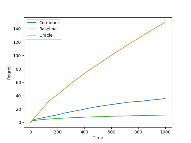
Figure 2: Model Selection Experiments

We now demonstrate empirical validation of our results in two different application settings. For our first experiment, we consider the misspecified linear bandit setting. We use ordinary UCB and linUCB as the two base algorithms. For simplicity we focus on the ordinary stochastic bandits framework (i.e. we assume the context remains fixed over time). Each arm a∈[K]a\in[K] is associated with a feature vector xa∈ℝdx_{a}\in\mathbb{R}^{d} that is chosen from the uniform distribution on the unit sphere. Let β∈ℝd\beta\in\mathbb{R}^{d} also chosen from the unit sphere be a fixed unknown parameter vector. Finally, for each arm aa, we choose μa∈ℝ\mu_{a}\in\mathbb{R} to be specified later. The reward for arm aa at any time step tt is set to be α​μa+(1−α)​d⋅⟨β,xa⟩+ηt\alpha\mu_{a}+(1-\alpha)\sqrt{d}\cdot\langle\beta,x_{a}\rangle+\eta_{t} where ηt∼𝒩⁡(0,σ)\eta_{t}\sim\mathcal{N}(0,\sigma) is independently sampled noise and 0≤α≤10\leq\alpha\leq 1 is a fixed constant. Let a⋆=argmina∈[K]⁡⟨β,xa⟩a^{\star}=\mathop{\text{argmin}}_{a\in[K]}\langle\beta,x_{a}\rangle be the worst arm with respect to the linear component of the reward. For any arm a≠a⋆a\neq a^{\star}, we set μa=0.25​d⋅⟨β,xa⟩\mu_{a}=0.25\sqrt{d}\cdot\langle\beta,x_{a}\rangle, whereas we set μa⋆=1\mu_{a^{\star}}=1. We consider two different settings of α\alpha. When α=0\alpha=0, the reward is simply a linear function of the arms and we expect the linUCB algorithm to outperform the ordinary UCB algorithm. On the other hand, when α=1\alpha=1, the rewards are constructed so that the linUCB algorithm essentially never chooses the arm a⋆a^{\star} and thus incurs linear regret whereas the ordinary UCB algorithm still guarantees O⁡(T)O(\sqrt{T}) regret. Figures 1(a) and 1(b) show the performance on these two settings respectively. In both settings, the combiner uses UCB and linUCB as the base algorithms and the putative regret bounds for UCB and linUCB are computed empirically on independent instances of the non-linear and linear reward settings respectively.

For our second experiment, we consider the model selection problem in linear bandits. As earlier, each arm a∈Ka\in K is associated with a feature vector xax_{a} sampled independently from the unit sphere. The parameter vector β∈ℝd\beta\in\mathbb{R}^{d} is chosen so that first each βj∼𝒩⁡(0,1),∀j≤d∗\beta_{j}\sim\mathcal{N}(0,1),\ \forall j\leq d^{*} and βj=0\beta_{j}=0, otherwise, and then normalized to be of unit length. The reward for arm aa at any time step tt is set to be ⟨β,xa⟩+ηt\langle\beta,x_{a}\rangle+\eta_{t} where as earlier ηt∼𝒩⁡(0,σ)\eta_{t}\sim\mathcal{N}(0,\sigma) is independently sampled noise. Figure 2 demonstrates the performance of three different algorithms in this setting with d=128,d∗=8d=128,d^{*}=8 and K=1000K=1000. The Baseline algorithm is a vanilla LinUCB algorithm that works on the ambient dimension dd, while the Oracle is a LinUCB algorithm that works on the true dimensionality of the reward parameter d∗d^{*}. The Combiner algorithm is an implementation of Algorithm 1 with log⁡d\log d base algorithms where each base algorithm AiA_{i} is an instance of LinUCB restricted to the first 2i2^{i} dimensions of the features. The putative regret bound CiC_{i} for each base algorithm AiA_{i} is computed empirically on independent instances where the corresponding algorithm is well-specified. We set the target regret bound Ri←(Ci2+N)​TR_{i}\leftarrow(C_{i}^{2}+N)\sqrt{T} where N=log⁡dN=\log d is the number of base algorithms. The experimental results validate our theoretical findings and show that the combiner algorithm is able to adapt to the true dimensionality of the rewards.

8 Conclusion

We have introduced a new method for combining stochastic bandit algorithms in such a way that our final regret may depend only on the regret of the best base algorithm in hindsight. Our method is based on upper-confidence techniques, and provides a contrast to prior work based on mirror descent [8]. We verify empirically that our technique can be used to solve some model selection and misspecification problems. In the future, we hope to see advancements in this area. For example, can we maintain logarithmic regret in benign settings? Further, in the full-information setting, one can often combine algorithms with minimal overhead. Are there any bandit settings in which such ideal behavior is possible?

References

  • [1] John Langford and Tong Zhang. The epoch-greedy algorithm for multi-armed bandits with side information. In Advances in neural information processing systems, pages 817–824, 2008.
  • [2] Alina Beygelzimer, John Langford, Lihong Li, Lev Reyzin, and Robert Schapire. Contextual bandit algorithms with supervised learning guarantees. In Proceedings of the Fourteenth International Conference on Artificial Intelligence and Statistics, pages 19–26, 2011.
  • [3] Tze Leung Lai and Herbert Robbins. Asymptotically efficient adaptive allocation rules. Advances in applied mathematics, 6(1):4–22, 1985.
  • [4] Peter Auer, Nicolo Cesa-Bianchi, and Paul Fischer. Finite-time analysis of the multiarmed bandit problem. Machine learning, 47(2-3):235–256, 2002.
  • [5] Tor Lattimore and Csaba Szepesvári. Bandit algorithms. preprint, page 28, 2018.
  • [6] Ambuj Tewari and Susan A Murphy. From ads to interventions: Contextual bandits in mobile health. In Mobile Health, pages 495–517. Springer, 2017.
  • [7] Alekh Agarwal, Daniel Hsu, Satyen Kale, John Langford, Lihong Li, and Robert Schapire. Taming the monster: A fast and simple algorithm for contextual bandits. In International Conference on Machine Learning, pages 1638–1646, 2014.
  • [8] Alekh Agarwal, Haipeng Luo, Behnam Neyshabur, and Robert E Schapire. Corralling a band of bandit algorithms. In Conference on Learning Theory, pages 12–38, 2017.
  • [9] Aldo Pacchiano, My Phan, Yasin Abbasi-Yadkori, Anup Rao, Julian Zimmert, Tor Lattimore, and Csaba Szepesvari. Model selection in contextual stochastic bandit problems. arXiv preprint arXiv:2003.01704, 2020.
  • [10] Sébastien Bubeck and Aleksandrs Slivkins. The best of both worlds: Stochastic and adversarial bandits. In Conference on Learning Theory, pages 42–1, 2012.
  • [11] Chen-Yu Wei and Haipeng Luo. More adaptive algorithms for adversarial bandits. Proceedings of Machine Learning Research, 75, 2018.
  • [12] Jean-Yves Audibert, Rémi Munos, and Csaba Szepesvári. Exploration–exploitation tradeoff using variance estimates in multi-armed bandits. Theoretical Computer Science, 410(19):1876–1902, 2009.
  • [13] Avishek Ghosh, Abishek Sankararaman, and Kannan Ramchandran. Problem-complexity adaptive model selection for stochastic linear bandits. arXiv preprint arXiv:2006.02612, 2020.
  • [14] Raman Arora, Teodor V Marinov, and Mehryar Mohri. Corralling stochastic bandit algorithms. arXiv preprint arXiv:2006.09255, 2020.
  • [15] Yasin Abbasi-Yadkori, Aldo Pacchiano, and My Phan. Regret balancing for bandit and rl model selection. arXiv preprint arXiv:2006.05491, 2020.
  • [16] Wei Chu, Lihong Li, Lev Reyzin, and Robert Schapire. Contextual bandits with linear payoff functions. In Proceedings of the Fourteenth International Conference on Artificial Intelligence and Statistics, pages 208–214, 2011.
  • [17] Tor Lattimore. The pareto regret frontier for bandits. In Advances in Neural Information Processing Systems, pages 208–216, 2015.
  • [18] Dylan J Foster, Akshay Krishnamurthy, and Haipeng Luo. Model selection for contextual bandits. In Advances in Neural Information Processing Systems, pages 14714–14725, 2019.
  • [19] Niladri S Chatterji, Vidya Muthukumar, and Peter L Bartlett. Osom: A simultaneously optimal algorithm for multi-armed and linear contextual bandits. arXiv preprint arXiv:1905.10040, 2019.
  • [20] Yasin Abbasi-Yadkori, Dávid Pál, and Csaba Szepesvári. Improved algorithms for linear stochastic bandits. In Advances in Neural Information Processing Systems, pages 2312–2320, 2011.
  • [21] Varsha Dani, Thomas P. Hayes, and Sham M. Kakade. Stochastic linear optimization under bandit feedback. In COLT, 2008.
  • [22] Sébastien Bubeck and Nicolò Cesa-Bianchi. Regret analysis of stochastic and nonstochastic multi-armed bandit problems. Foundations and Trends in Machine Learning, 5(1):1–122, 2012.
  • [23] Aleksandrs Slivkins. Introduction to multi-armed bandits. Foundations and Trends in Machine Learning, 12(1-2):1–286, 2019.
  • [24] Yasin Abbasi-Yadkori, David Pal, and Csaba Szepesvari. Online-to-confidence-set conversions and application to sparse stochastic bandits. In Artificial Intelligence and Statistics, pages 1–9, 2012.
  • [25] H Brendan McMahan. A survey of algorithms and analysis for adaptive online learning. The Journal of Machine Learning Research, 18(1):3117–3166, 2017.
  • [26] Elad Hazan, Amit Agarwal, and Satyen Kale. Logarithmic regret algorithms for online convex optimization. Machine Learning, 69(2-3):169–192, 2007.

Appendix A Lemmas for analysis of Algorithm 1

Before proving Theorem 1, we need a few Lemmas. For the most part, these are straightforward verification of intuitive concentration bounds.

Lemma 8.

With probability at least 1−δ/T≥1−δ1-\delta/T\geq 1-\delta, for all ii, for all tt, we have:

∑τ=1T⁡(i,t)rτi−r^τi≤8​log⁡(T3​N/δ)​T​(i,t)\displaystyle\sum_{\tau=1}^{T(i,t)}r^{i}_{\tau}-\hat{r}^{i}_{\tau}\leq\sqrt{8\log(T^{3}N/\delta)T(i,t)}

Similarly, with probability at least 1−δ1-\delta, for all ii, for all tt, we have:

∑τ=1T⁡(i,t)r^τi−rτi≤8​log⁡(T3​N/δ)​T​(i,t)\displaystyle\sum_{\tau=1}^{T(i,t)}\hat{r}^{i}_{\tau}-r^{i}_{\tau}\leq\sqrt{8\log(T^{3}N/\delta)T(i,t)}
Proof.

We prove only the first statement. The proof of the second is entirely symmetrical.

Fix a given ii. For any τ≤T\tau\leq T define zτ=rτi−r^τiz_{\tau}=r^{i}_{\tau}-\hat{r}^{i}_{\tau}, we recall that rτir^{i}_{\tau} is the expected value of the τ\tauth action of AiA_{i} given the past history - if tt is the first time that T⁡(i,t)=τT(i,t)=\tau, we have rτi=𝔼[r^τi|r^1,…,r^t−1]r^{i}_{\tau}=\mathop{\mathbb{E}}[\hat{r}^{i}_{\tau}|\hat{r}_{1},\dots,\hat{r}_{t-1}]. Notice that zτ∈[−1,1]z_{\tau}\in[-1,1] is a martingale difference sequence.

Now for any ϵ\epsilon we apply Azuma’s inequality to obtain for any tt:

Prob[∑τ=1trτi−r^τi≥ϵ]\displaystyle\text{Prob}\left[\sum_{\tau=1}^{t}r^{i}_{\tau}-\hat{r}^{i}_{\tau}\geq\epsilon\right] =Prob[∑τ=1tzτ≥ϵ]\displaystyle=\text{Prob}\left[\sum_{\tau=1}^{t}z_{\tau}\geq\epsilon\right]
≤exp⁡(−ϵ28​t)\displaystyle\leq\exp\left(\frac{-\epsilon^{2}}{8t}\right)

In particular, setting ϵ=8​t​log⁡(T3​N/δ)\epsilon=\sqrt{8t\log(T^{3}N/\delta)}, we have that

Prob[∑τ=1trτi−r^τi≥8​log⁡(T3​N/δ)​t]≤δT3​N\displaystyle\text{Prob}\left[\sum_{\tau=1}^{t}r^{i}_{\tau}-\hat{r}^{i}_{\tau}\geq\sqrt{8\log(T^{3}N/\delta)t}\right]\leq\frac{\delta}{T^{3}N}

Therefore:

Prob[∑τ=1T⁡(i,t)rτi−r^τi≥8​log⁡(T3​N/δ)​T​(i,t)]\displaystyle\text{Prob}\left[\sum_{\tau=1}^{T(i,t)}r^{i}_{\tau}-\hat{r}^{i}_{\tau}\geq\sqrt{8\log(T^{3}N/\delta)T(i,t)}\right] =∑t′=1TProb[∑τ=1t′rτi−r^τi≥8​log⁡(T3​N/δ)​t′ and T(i,t)=t′]\displaystyle=\sum_{t^{\prime}=1}^{T}\text{Prob}\left[\sum_{\tau=1}^{t^{\prime}}r^{i}_{\tau}-\hat{r}^{i}_{\tau}\geq\sqrt{8\log(T^{3}N/\delta)t^{\prime}}\text{ and }T(i,t)=t^{\prime}\right]
≤∑t′=1TProb[∑τ=1t′rτi−r^τi≥8​log⁡(T3​N/δ)​t′]\displaystyle\leq\sum_{t^{\prime}=1}^{T}\text{Prob}\left[\sum_{\tau=1}^{t^{\prime}}r^{i}_{\tau}-\hat{r}^{i}_{\tau}\geq\sqrt{8\log(T^{3}N/\delta)t^{\prime}}\right]
≤δN​T2\displaystyle\leq\frac{\delta}{NT^{2}}

Then union bound over the NN indices ii and TT values of tt completes the Lemma. ∎

Similarly, we have the following result:

Lemma 9.

With probability at least 1−δ1-\delta, for all ii, for all tt, we have:

∑τ=1T⁡(i,t)μ^τi−r⋆≤2​8​log⁡(T3​N/δ)​T​(i,t)\displaystyle\sum_{\tau=1}^{T(i,t)}\hat{\mu}^{i}_{\tau}-r_{\star}\leq 2\sqrt{8\log(T^{3}N/\delta)T(i,t)}
Proof.

Following the same argument as in Lemma 8, we have that for any ii and tt,

Prob[∑τ=1tr^τi−rτi≥8​log⁡(T3​N/δ)​t]≤δT3​N\displaystyle\text{Prob}\left[\sum_{\tau=1}^{t}\hat{r}^{i}_{\tau}-r^{i}_{\tau}\geq\sqrt{8\log(T^{3}N/\delta)t}\right]\leq\frac{\delta}{T^{3}N}

Further, note that since rti≤r⋆r^{i}_{t}\leq r_{\star} for all ii and tt, ∑τ=1tr^τi−rτi≤8​log⁡(T3​N/δ)​t\sum_{\tau=1}^{t}\hat{r}^{i}_{\tau}-r^{i}_{\tau}\leq\sqrt{8\log(T^{3}N/\delta)t} implies μ^ti−r⋆≤8​log⁡(T3​N/δ)t\hat{\mu}^{i}_{t}-r_{\star}\leq\frac{\sqrt{8\log(T^{3}N/\delta)}}{\sqrt{t}}. Therefore, for any ii and tt,

Prob[μ^ti−r⋆≥8​log⁡(T3​N/δ)t]≤δT3​N\displaystyle\text{Prob}\left[\hat{\mu}^{i}_{t}-r_{\star}\geq\frac{\sqrt{8\log(T^{3}N/\delta)}}{\sqrt{t}}\right]\leq\frac{\delta}{T^{3}N}

Further, observe that if μ^ti−r⋆≤8​log⁡(T3​N/δ)t\hat{\mu}^{i}_{t}-r_{\star}\leq\frac{\sqrt{8\log(T^{3}N/\delta)}}{\sqrt{t}} for all tt, then ∑^τ=1t​μτi−r⋆≤2​8​log⁡(T3​N/δ)​t\hat{\sum}_{\tau=1}^{t}\mu^{i}_{\tau}-r_{\star}\leq 2\sqrt{8\log(T^{3}N/\delta)t}. Therefore for any given tt and ii:

Prob[∑τ=1T⁡(i,t)μ^τi−r⋆≥28​log⁡(T3​N/δ)T⁡(i,t)]\displaystyle\text{Prob}\left[\sum_{\tau=1}^{T(i,t)}\hat{\mu}^{i}_{\tau}-r_{\star}\geq 2\sqrt{8\log(T^{3}N/\delta)}\sqrt{T(i,t)}\right] =∑t′=1TProb[∑τ=1t′μ^τi−r⋆≥28​log⁡(T3​N/δ)t′ and T(i,t)=t′]\displaystyle=\sum_{t^{\prime}=1}^{T}\text{Prob}\left[\sum_{\tau=1}^{t^{\prime}}\hat{\mu}^{i}_{\tau}-r_{\star}\geq 2\sqrt{8\log(T^{3}N/\delta)}\sqrt{t^{\prime}}\text{ and }T(i,t)=t^{\prime}\right]
≤∑t′=1TProb[∑τ=1t′μ^τi−r⋆≥28​log⁡(T3​N/δ)t′]\displaystyle\leq\sum_{t^{\prime}=1}^{T}\text{Prob}\left[\sum_{\tau=1}^{t^{\prime}}\hat{\mu}^{i}_{\tau}-r_{\star}\geq 2\sqrt{8\log(T^{3}N/\delta)}\sqrt{t^{\prime}}\right]
≤∑t′=1TProb[μ^τi−r⋆≤8​log⁡(T3​N/δ)τ for all τ≤t′]\displaystyle\leq\sum_{t^{\prime}=1}^{T}\text{Prob}\left[\hat{\mu}^{i}_{\tau}-r_{\star}\leq\frac{\sqrt{8\log(T^{3}N/\delta)}}{\sqrt{\tau}}\text{ for all }\tau\leq t^{\prime}\right]
≤∑t′=1T∑τ=1t′Prob[μ^τi−r⋆≤8​log⁡(T3​N/δ)τ]\displaystyle\leq\sum_{t^{\prime}=1}^{T}\sum_{\tau=1}^{t^{\prime}}\text{Prob}\left[\hat{\mu}^{i}_{\tau}-r_{\star}\leq\frac{\sqrt{8\log(T^{3}N/\delta)}}{\sqrt{\tau}}\right]
≤δT​N\displaystyle\leq\frac{\delta}{TN}

Now a union bound over the TT values of tt and NN values of ii completes the statement. ∎

Lemma 10.

With probability at least 1−3​δ1-3\delta, there is some J∈SJ\in S such that for all tt we have simultaneously:

∑τ=1T⁡(J,t)r⋆−r^τJ\displaystyle\sum_{\tau=1}^{T(J,t)}r_{\star}-\hat{r}^{J}_{\tau} ≤CJ​T​(J,t)αJ\displaystyle\leq C_{J}T(J,t)^{\alpha_{J}}
r⋆−μ^T⁡(i,t−1)J\displaystyle r_{\star}-\hat{\mu}^{J}_{T(i,t-1)} ≤min⁡(1,CJ​T​(J,t−1)αJ−1+8​log⁡(T3​N/δ)T⁡(J,t−1))\displaystyle\leq\min\left(1,C_{J}T(J,t-1)^{\alpha_{J}-1}+\frac{\sqrt{8\log(T^{3}N/\delta)}}{\sqrt{T(J,t-1)}}\right)
∑τ=1T⁡(J,t−1)μ^τ−1J−r^τJ\displaystyle\sum_{\tau=1}^{T(J,t-1)}\hat{\mu}^{J}_{\tau-1}-\hat{r}^{J}_{\tau} ≤CJ​T​(J,t−1)αJ+3​8​log⁡(T​N/δ)​T​(J,t−1)\displaystyle\leq C_{J}T(J,t-1)^{\alpha_{J}}+3\sqrt{8\log(TN/\delta)T(J,t-1)}
Proof.

By assumption, with probability 1−δ1-\delta we have that there is some J∈SJ\in S such that for all tt,

∑t=1T⁡(J,t−1)r⋆−rτJ≤CJ​T​(J,t−1)αJ\displaystyle\sum_{t=1}^{T(J,t-1)}r_{\star}-r^{J}_{\tau}\leq C_{J}T(J,t-1)^{\alpha_{J}} (4)

Next, by Lemma 8 we have with probability at least 1−δ1-\delta, for all tt,

∑τ=1T⁡(J,t−1)rτJ−r^τJ≤8​log⁡(T3​N/δ)​T​(J,t−1)\displaystyle\sum_{\tau=1}^{T(J,t-1)}r^{J}_{\tau}-\hat{r}^{J}_{\tau}\leq\sqrt{8\log(T^{3}N/\delta)T(J,t-1)} (5)

and by Lemma 9, with probability 1−δ1-\delta we have for all tt:

∑τ=1T⁡(J,t)μ^τJ−r⋆≤2​8​log⁡(T3​N/δ)​T​(J,t)\displaystyle\sum_{\tau=1}^{T(J,t)}\hat{\mu}^{J}_{\tau}-r_{\star}\leq 2\sqrt{8\log(T^{3}N/\delta)T(J,t)} (6)

All three equations then hold with probability at least 1−3​δ1-3\delta. Let us condition on this probability 1−3​δ1-3\delta event. Then the first equation in the Lemma is immediately satisfied.

For the second equation, observe that since μ^T⁡(J,t−1)J\hat{\mu}^{J}_{T(J,t-1)} and r⋆r_{\star} are both in [0,1][0,1], the statement is true so long as the minimum binds to 1. Further, for T⁡(J,t−1)≠0T(J,t-1)\neq 0, we have

r⋆−μ^T⁡(J,t−1)J\displaystyle r_{\star}-\hat{\mu}^{J}_{T(J,t-1)} =1T⁡(J,t−1)​∑τ=1T⁡(J,t−1)r⋆−r^τJ\displaystyle=\frac{1}{T(J,t-1)}\sum_{\tau=1}^{T(J,t-1)}r_{\star}-\hat{r}^{J}_{\tau}
=1T⁡(J,t−1)​∑τ=1T⁡(J,t−1)r⋆−rτJ+1T⁡(J,t−1)​∑τ=1T⁡(J,t−1)rτJ−r^τJ\displaystyle=\frac{1}{T(J,t-1)}\sum_{\tau=1}^{T(J,t-1)}r_{\star}-r^{J}_{\tau}+\frac{1}{T(J,t-1)}\sum_{\tau=1}^{T(J,t-1)}r^{J}_{\tau}-\hat{r}^{J}_{\tau}
≤CJ​T​(J,t−1)αJ−1+8​log⁡(T3​N/δ)T⁡(J,t−1)\displaystyle\leq C_{J}T(J,t-1)^{\alpha_{J}-1}+\frac{\sqrt{8\log(T^{3}N/\delta)}}{\sqrt{T(J,t-1)}}

Now for the third equation, observe μ^0J=0\hat{\mu}^{J}_{0}=0, so that

∑τ=1T⁡(J,t−1)μ^τ−1i−r⋆\displaystyle\sum_{\tau=1}^{T(J,t-1)}\hat{\mu}^{i}_{\tau-1}-r_{\star} ≤∑τ=1T⁡(J,t−1)μ^τi−r⋆\displaystyle\leq\sum_{\tau=1}^{T(J,t-1)}\hat{\mu}^{i}_{\tau}-r_{\star}
≤∑τ=1T⁡(J,t−1)8​log⁡(T3​N/δ)τ\displaystyle\leq\sum_{\tau=1}^{T(J,t-1)}\frac{\sqrt{8\log(T^{3}N/\delta)}}{\sqrt{\tau}}
≤2​8​log⁡(T3​N/δ)​T​(J,t−1)\displaystyle\leq 2\sqrt{8\log(T^{3}N/\delta)T(J,t-1)}

Combining these equations yields:

∑τ=1T⁡(J,t−1)μ^τ−1J−r^τJ\displaystyle\sum_{\tau=1}^{T(J,t-1)}\hat{\mu}^{J}_{\tau-1}-\hat{r}^{J}_{\tau} =∑τ=1T⁡(J,t−1)μ^τ−1J−r⋆+r⋆−rτJ+rτJ−r^τJ\displaystyle=\sum_{\tau=1}^{T(J,t-1)}\hat{\mu}^{J}_{\tau-1}-r_{\star}+r_{\star}-r^{J}_{\tau}+r^{J}_{\tau}-\hat{r}^{J}_{\tau}
≤2​8​log⁡(T3​N/δ)​T​(J,t−1)+CJ​T​(J,t−1)αJ+8​log⁡(T3​N/δ)​T​(J,t−1)\displaystyle\leq 2\sqrt{8\log(T^{3}N/\delta)T(J,t-1)}+C_{J}T(J,t-1)^{\alpha_{J}}+\sqrt{8\log(T^{3}N/\delta)T(J,t-1)}
≤CJ​T​(J,t−1)αJ+3​8​log⁡(T3​N/δ)​T​(J,t−1)\displaystyle\leq C_{J}T(J,t-1)^{\alpha_{J}}+3\sqrt{8\log(T^{3}N/\delta)T(J,t-1)}

∎

We also need a bound on the performance of the misspecified algorithms:

Lemma 11.

With probability at least 1−δ1-\delta, all indices ii satisfy:

∑τ=1T⁡(i,T)μ^τ−1i−rτi≤Ci​T​(i,T)αi+4​8​log⁡(T​N/δ)​T​(i,T)+1\displaystyle\sum_{\tau=1}^{T(i,T)}\hat{\mu}^{i}_{\tau-1}-r^{i}_{\tau}\leq C_{i}T(i,T)^{\alpha_{i}}+4\sqrt{8\log(TN/\delta)T(i,T)}+1
Proof.

Let tt be the smallest time such that T⁡(i,t)=T⁡(i,T)T(i,t)=T(i,T). Then it=ii_{t}=i, so we must have that i∈Iti\in I_{t}. Therefore:

∑τ=1T⁡(i,t−1)μ^τ−1i−r^τi≤Ci​T​(i,t−1)αi+3​8​log⁡(T3​N/δ)​(T⁡(i,t−1))\displaystyle\sum_{\tau=1}^{T(i,t-1)}\hat{\mu}^{i}_{\tau-1}-\hat{r}^{i}_{\tau}\leq C_{i}T(i,t-1)^{\alpha_{i}}+3\sqrt{8\log(T^{3}N/\delta)(T(i,t-1))}

Next, by Lemma 8, we have that with probability at least 1−δ1-\delta,

∑τ=1T⁡(i,t−1)r^τi−rτi\displaystyle\sum_{\tau=1}^{T(i,t-1)}\hat{r}^{i}_{\tau}-r^{i}_{\tau} ≤8​log⁡(T3​N/δ)​T​(i,t−1)\displaystyle\leq\sqrt{8\log(T^{3}N/\delta)T(i,t-1)}

Then observe that since all rewards are in [0,1][0,1], we must have μ^T⁡(i,t)−1i−rT⁡(i,t)i≤1\hat{\mu}^{i}_{T(i,t)-1}-r^{i}_{T(i,t)}\leq 1 and the statement follows. ∎

One more technical fact:

Lemma 12.

Suppose α∈[1/2,1)\alpha\in[1/2,1). Then for any constants A,B≥0A,B\geq 0,

supZ≥0A​Zα−B​Z\displaystyle\sup_{Z\geq 0}AZ^{\alpha}-BZ =αα1−α​(1−α)​A11−αBα1−α\displaystyle=\alpha^{\frac{\alpha}{1-\alpha}}\left(1-\alpha\right)\frac{A^{\frac{1}{1-\alpha}}}{B^{\frac{\alpha}{1-\alpha}}}
Proof.

We differentiate with respect to ZZ to obtain:

α​A​Zα−1\displaystyle\alpha AZ^{\alpha-1} =B\displaystyle=B
Z\displaystyle Z =(α​AB)11−α\displaystyle=\left(\frac{\alpha A}{B}\right)^{\frac{1}{1-\alpha}}
Now substitute this value back into the original expression:
A​Xα−B​X\displaystyle AX^{\alpha}-BX =(αα1−α−α11−α)​A11−αBα1−α\displaystyle=\left(\alpha^{\frac{\alpha}{1-\alpha}}-\alpha^{\frac{1}{1-\alpha}}\right)\frac{A^{\frac{1}{1-\alpha}}}{B^{\frac{\alpha}{1-\alpha}}}
=αα1−α​(1−α)​A11−αBα1−α\displaystyle=\alpha^{\frac{\alpha}{1-\alpha}}\left(1-\alpha\right)\frac{A^{\frac{1}{1-\alpha}}}{B^{\frac{\alpha}{1-\alpha}}}

∎

Appendix B Proof of Theorem 1

Now we are in a position to prove Theorem 1, which we restate below for reference: See 1

Proof.

To begin, observe that by Lemma 10 and Lemma 11, with probability 1−4​δ1-4\delta, there is some J∈SJ\in S such that for all tt and all ii, we have

∑τ=1T⁡(J,T)r⋆−rτJ\displaystyle\sum_{\tau=1}^{T(J,T)}r_{\star}-r^{J}_{\tau} ≤CJ​T​(J,T)αJ\displaystyle\leq C_{J}T(J,T)^{\alpha_{J}} (7)
r⋆−μ^T⁡(J,t−1)J\displaystyle r_{\star}-\hat{\mu}^{J}_{T(J,t-1)} ≤min⁡(1,CJ​T​(J,t−1)αJ−1+8​log⁡(T3​N/δ)T⁡(J,t−1))\displaystyle\leq\min\left(1,C_{J}T(J,t-1)^{\alpha_{J}-1}+\frac{\sqrt{8\log(T^{3}N/\delta)}}{\sqrt{T(J,t-1)}}\right) (8)
J\displaystyle J ∈It\displaystyle\in I_{t}
∑τ=1T⁡(i,T)μ^τ−1i−rτi\displaystyle\sum_{\tau=1}^{T(i,T)}\hat{\mu}^{i}_{\tau-1}-r^{i}_{\tau} ≤Ci​T​(i,T)αi+4​8​log⁡(T​N/δ)​T​(i,T)+1\displaystyle\leq C_{i}T(i,T)^{\alpha_{i}}+4\sqrt{8\log(TN/\delta)T(i,T)}+1 (9)

All of our analysis is conditioned on this probability 1−4​δ1-4\delta event.

First, notice that by (8), we have that we have that:

r⋆\displaystyle r_{\star} ≤U⁡(J,t−1)+RJT\displaystyle\leq U(J,t-1)+\frac{R_{J}}{T}

for all tt.

Now we write the regret:

∑t=1Tr⋆−rt\displaystyle\sum_{t=1}^{T}r_{\star}-r_{t} =∑t=1Tr⋆−rT⁡(it,t)it\displaystyle=\sum_{t=1}^{T}r_{\star}-r^{i_{t}}_{T(i_{t},t)}
=∑it=Jr⋆−rT⁡(J,t)J+∑it≠Jr⋆−rT⁡(it,t)it\displaystyle=\sum_{i_{t}=J}r_{\star}-r^{J}_{T(J,t)}+\sum_{i_{t}\neq J}r_{\star}-r^{i_{t}}_{T(i_{t},t)}

First let’s consider the indices for which it=Ji_{t}=J:

∑it=Jr⋆−rT⁡(J,t)J≤CJ​T​(J,T)αJ≤RJ\displaystyle\sum_{i_{t}=J}r_{\star}-r^{J}_{T(J,t)}\leq C_{J}T(J,T)^{\alpha_{J}}\leq R_{J}

Next, if it≠Ji_{t}\neq J, we must have U⁡(it,t−1)≥U⁡(J,t−1)U(i_{t},t-1)\geq U(J,t-1) since J∈ItJ\in I_{t} for all tt. Then:

r⋆\displaystyle r_{\star} =r⋆−U⁡(J,t−1)+U⁡(J,t−1)−U⁡(it,t−1)+U⁡(it,t−1)\displaystyle=r_{\star}-U(J,t-1)+U(J,t-1)-U(i_{t},t-1)+U(i_{t},t-1)
≤RJT+U⁡(it,t−1)\displaystyle\leq\frac{R_{J}}{T}+U(i_{t},t-1)

Therefore:

∑it≠Jr⋆−rT⁡(it,t)it\displaystyle\sum_{i_{t}\neq J}r_{\star}-r^{i_{t}}_{T(i_{t},t)} ≤∑it≠JRJT+U⁡(it,t−1)−rT⁡(it,t)it\displaystyle\leq\sum_{i_{t}\neq J}\frac{R_{J}}{T}+U(i_{t},t-1)-r^{i_{t}}_{T(i_{t},t)}
≤RJ+∑it≠JU⁡(it,t−1)−rT⁡(it,t)it\displaystyle\leq R_{J}+\sum_{i_{t}\neq J}U(i_{t},t-1)-r^{i_{t}}_{T(i_{t},t)}

Let us focus on the sum ∑it≠JU⁡(it,t−1)−rT⁡(it,t)it\sum_{i_{t}\neq J}U(i_{t},t-1)-r^{i_{t}}_{T(i_{t},t)}. As a first step, we observe the following identity:

∑t|it=iU⁡(i,t−1)−μ^T⁡(i,t−1)i\displaystyle\sum_{t\ |\ i_{t}=i}U(i,t-1)-\hat{\mu}^{i}_{T(i,t-1)} =∑τ=1T⁡(i,T)min⁡(1,Ci​(τ−1)αi−1+8​log⁡(T3​N/δ)τ−1)−RiT\displaystyle=\sum_{\tau=1}^{T(i,T)}\min\left(1,C_{i}(\tau-1)^{\alpha_{i}-1}+\frac{\sqrt{8\log(T^{3}N/\delta)}}{\sqrt{\tau-1}}\right)-\frac{R_{i}}{T}
≤1−T⁡(i,T)​RiT+∑τ=1T⁡(i,T)Ci​ταi−1+8​log⁡(T3​N/δ)τ\displaystyle\leq 1-\frac{T(i,T)R_{i}}{T}+\sum_{\tau=1}^{T(i,T)}C_{i}\tau^{\alpha_{i}-1}+\frac{\sqrt{8\log(T^{3}N/\delta)}}{\sqrt{\tau}}
≤1−T⁡(i,T)​RiT+Ci​T​(i,T)αiαi+2​8​log⁡(T3​N/δ)​T​(i,T)\displaystyle\leq 1-\frac{T(i,T)R_{i}}{T}+\frac{C_{i}T(i,T)^{\alpha_{i}}}{\alpha_{i}}+2\sqrt{8\log(T^{3}N/\delta)T(i,T)}

Now we use this observation as follows:

∑it≠JU⁡(it,t−1)−r^T⁡(it,t)it\displaystyle\sum_{i_{t}\neq J}U(i_{t},t-1)-\hat{r}^{i_{t}}_{T(i_{t},t)} =∑it≠Jμ^T⁡(it,t−1)it−rT⁡(it,t)it+U⁡(it,t−1)−μ^T⁡(it,t−1)it\displaystyle=\sum_{i_{t}\neq J}\hat{\mu}^{i_{t}}_{T(i_{t},t-1)}-r^{i_{t}}_{T(i_{t},t)}+U(i_{t},t-1)-\hat{\mu}^{i_{t}}_{T(i_{t},t-1)}
≤∑i≠J[∑t|it=iμ^T⁡(i,t−1)i−rT⁡(it,t)it+U⁡(i,t−1)−μ^T⁡(i,t−1)i]\displaystyle\leq\sum_{i\neq J}\left[\sum_{t\ |\ i_{t}=i}\hat{\mu}^{i}_{T(i,t-1)}-r^{i_{t}}_{T(i_{t},t)}+U(i,t-1)-\hat{\mu}^{i}_{T(i,t-1)}\right]
≤∑i≠J1−T⁡(i,T)​RiT+Ci​T​(i,T)αiαi+2​8​log⁡(T3​N/δ)​T​(i,T)+∑τ=1T⁡(i,T)μ^τ−1i−rτi\displaystyle\leq\sum_{i\neq J}1-\frac{T(i,T)R_{i}}{T}+\frac{C_{i}T(i,T)^{\alpha_{i}}}{\alpha_{i}}+2\sqrt{8\log(T^{3}N/\delta)T(i,T)}+\sum_{\tau=1}^{T(i,T)}\hat{\mu}^{i}_{\tau-1}-r^{i}_{\tau}
≤∑i≠J−T⁡(i,T)​RiT+Ci​T​(i,T)αiαi+38​log⁡(T3​N/δ)​T​(i,T)+∑τ=1T⁡(i,T)μ^iτ−1−riτ\displaystyle\leq\sum_{i\neq J}-\frac{T(i,T)R_{i}}{T}+\frac{C_{i}T(i,T)^{\alpha_{i}}}{\alpha_{i}}+3\sqrt{8\log(T^{3}N/\delta)T(i,T)}+\sum_{\tau=1}^{T(i,T)}\hat{\mu}^{i}_{\tau-1}-r^{i}_{\tau}
≤∑i≠J(1+αi)​Ci​T​(i,T)αiαi+6​8​log⁡(T3​N/δ)​T​(i,T)−T⁡(i,T)​RiT\displaystyle\leq\sum_{i\neq J}\frac{(1+\alpha_{i})C_{i}T(i,T)^{\alpha_{i}}}{\alpha_{i}}+6\sqrt{8\log(T^{3}N/\delta)T(i,T)}-\frac{T(i,T)R_{i}}{T}

Now we use a simple trick that allows us to apply Lemma 12:

(1+αi)​Ci​T​(i,T)αiαi+6​8​log⁡(T3​N/δ)​T​(i,T)−T⁡(i,T)​RiT\displaystyle\frac{(1+\alpha_{i})C_{i}T(i,T)^{\alpha_{i}}}{\alpha_{i}}+6\sqrt{8\log(T^{3}N/\delta)T(i,T)}-\frac{T(i,T)R_{i}}{T}
≤supZ(1+αi)​Ci​Zαiαi+6​8​log⁡(T3​N/δ)​Z−Z​RiT\displaystyle\leq\sup_{Z}\frac{(1+\alpha_{i})C_{i}Z^{\alpha_{i}}}{\alpha_{i}}+6\sqrt{8\log(T^{3}N/\delta)Z}-\frac{ZR_{i}}{T}
≤max⁡[supZ(1+αi)​2​Ci​Zαiαi−Z​RiT,supZ12​8​log⁡(T3​N/δ)​Z−Z​RiT]\displaystyle\leq\max\left[\sup_{Z}\frac{(1+\alpha_{i})2C_{i}Z^{\alpha_{i}}}{\alpha_{i}}-\frac{ZR_{i}}{T},\sup_{Z}12\sqrt{8\log(T^{3}N/\delta)Z}-\frac{ZR_{i}}{T}\right]
≤max⁡[(1−αi)​(1+αi)11−αi​(2​Ci)11−αi​Tαi1−αiαi​Rαi1−αi,288​log⁡(T3​N/δ)​TRi]\displaystyle\leq\max\left[\frac{(1-\alpha_{i})(1+\alpha_{i})^{\frac{1}{1-\alpha_{i}}}(2C_{i})^{\frac{1}{1-\alpha_{i}}}T^{\frac{\alpha_{i}}{1-\alpha_{i}}}}{\alpha_{i}R^{\frac{\alpha_{i}}{1-\alpha_{i}}}},\frac{288\log(T^{3}N/\delta)T}{R_{i}}\right]

Therefore by our conditions on the RiR_{i}, we have

∑i≠J(1+αi)​Ci​T​(i,T)αiαi+6​8​log⁡(T3​N/δ)​T​(i,T)−T⁡(i,T)​RiT\displaystyle\sum_{i\neq J}\frac{(1+\alpha_{i})C_{i}T(i,T)^{\alpha_{i}}}{\alpha_{i}}+6\sqrt{8\log(T^{3}N/\delta)T(i,T)}-\frac{T(i,T)R_{i}}{T}
≤∑i≠Jmax⁡[(1−αi)​(1+αi)11−αi​(2​Ci)11−αi​Tαi1−αiαi​Rαi1−αi,288​log⁡(T3​N/δ)​TRi]\displaystyle\leq\sum_{i\neq J}\max\left[\frac{(1-\alpha_{i})(1+\alpha_{i})^{\frac{1}{1-\alpha_{i}}}(2C_{i})^{\frac{1}{1-\alpha_{i}}}T^{\frac{\alpha_{i}}{1-\alpha_{i}}}}{\alpha_{i}R^{\frac{\alpha_{i}}{1-\alpha_{i}}}},\frac{288\log(T^{3}N/\delta)T}{R_{i}}\right]
≤RJ\displaystyle\leq R_{J}

And so putting all this together we have with probability at least 1−3​δ1-3\delta:

∑t=1Tr⋆−r^t\displaystyle\sum_{t=1}^{T}r_{\star}-\hat{r}_{t} =∑it=Jr⋆−r^T⁡(J,t)J+∑it≠Jr⋆−r^T⁡(it,t)it\displaystyle=\sum_{i_{t}=J}r_{\star}-\hat{r}^{J}_{T(J,t)}+\sum_{i_{t}\neq J}r_{\star}-\hat{r}^{i_{t}}_{T(i_{t},t)}
≤RJ+RJ+RJ≤3​RJ\displaystyle\leq R_{J}+R_{J}+R_{J}\leq 3R_{J}

for some J∈SJ\in S. Therefore with probability at least 1−3​δ1-3\delta, the regret is bounded by 3​supj∈SRj3\sup_{j\in S}R_{j}. ∎

B.1 Proof of Corollary 2

Now we prove Corollary 2: See 2

Proof.

Observe that by definition of RiR_{i} we have:

Ri\displaystyle R_{i} ≥Ci​Tαi\displaystyle\geq C_{i}T^{\alpha_{i}}
Further, due to the second and third terms in the definition of RiR_{i} respectively, we have the following:
1ηi\displaystyle\frac{1}{\eta_{i}} ≥(1−αi)​(1+αi)11−αi​(2​Ci)11−αi​Tαi1−αiαi​Riαi1−αi\displaystyle\geq\frac{(1-\alpha_{i})(1+\alpha_{i})^{\frac{1}{1-\alpha_{i}}}(2C_{i})^{\frac{1}{1-\alpha_{i}}}T^{\frac{\alpha_{i}}{1-\alpha_{i}}}}{\alpha_{i}R_{i}^{\frac{\alpha_{i}}{1-\alpha_{i}}}}
1ηi\displaystyle\frac{1}{\eta_{i}} ≥288​log⁡(T3​N/δ)​TRi\displaystyle\geq\frac{288\log(T^{3}N/\delta)T}{R_{i}}
Finally, due to the last term in the definition of RiR_{i}, we have:
Ri\displaystyle R_{i} ≥∑k≠i1ηk\displaystyle\geq\sum_{k\neq i}\frac{1}{\eta_{k}}
≥∑k≠imax⁡{(1−αk)​(1+αk)11−αk​(2​Ck)11−αk​Tαk1−αkαk​Rkαk1−αk,288​log⁡(T3​N/δ)​TRk}\displaystyle\geq\sum_{k\neq i}\max\left\{\frac{(1-\alpha_{k})(1+\alpha_{k})^{\frac{1}{1-\alpha_{k}}}(2C_{k})^{\frac{1}{1-\alpha_{k}}}T^{\frac{\alpha_{k}}{1-\alpha_{k}}}}{\alpha_{k}R_{k}^{\frac{\alpha_{k}}{1-\alpha_{k}}}},\frac{288\log(T^{3}N/\delta)T}{R_{k}}\right\}

Therefore these RiR_{i} satisfy the conditions of Theorem 1, and so we are done. ∎

Appendix C Proof of Theorem 3

See 3

Proof.

We begin with the regret decomposition:

∑t=1Tr⋆−rt=∑τ=1T⁡(J,T)r⋆−rτJ+∑i∉B,i≠J∑τ=1T⁡(i,T)r⋆−rτi+∑i∈B∑τ=1T⁡(i,T)r⋆−rτi\displaystyle\sum_{t=1}^{T}r_{\star}-r_{t}=\sum_{\tau=1}^{T(J,T)}r_{\star}-r^{J}_{\tau}+\sum_{i\notin B,i\neq J}\sum_{\tau=1}^{T(i,T)}r_{\star}-r^{i}_{\tau}+\sum_{i\in B}\sum_{\tau=1}^{T(i,T)}r_{\star}-r^{i}_{\tau}

The first sum in the above is already in the form we desire. The second sum could be bounded using the same argument as in the proof of Theorem 1 by:

RJ+∑k≠J,k∉Bmax⁡[(1−αk)​(1+αk)11−αk​(2​Ck)11−αk​Tαk1−αkαk​Rkαk1−αk,288​log⁡(T3​N/δ)​TRk]\displaystyle R_{J}+\sum_{k\neq J,k\notin B}\max\left[\frac{(1-\alpha_{k})(1+\alpha_{k})^{\frac{1}{1-\alpha_{k}}}(2C_{k})^{\frac{1}{1-\alpha_{k}}}T^{\frac{\alpha_{k}}{1-\alpha_{k}}}}{\alpha_{k}R_{k}^{\frac{\alpha_{k}}{1-\alpha_{k}}}},\ \frac{288\log(T^{3}N/\delta)T}{R_{k}}\right]

However, we can also bound it another way. By definition of BB, for any i∉Bi\notin B, we have:

∑τ=1T⁡(i,T)r⋆−rτi≤T​Δi≤2​RJ\displaystyle\sum_{\tau=1}^{T(i,T)}r_{\star}-r^{i}_{\tau}\leq T\Delta_{i}\leq 2R_{J}

so that the second sum is also bounded by

∑k≠J,k∉B2​RJ\displaystyle\sum_{k\neq J,k\notin B}2R_{J}

This leads to the expression involving a minimum in the Theorem statement.

For the last term, our proof proceeds by counting how many times we choose an algorithm 𝒜i\mathcal{A}_{i} for i∈Bi\in B. We only choose such an algorithm when U⁡(i,t−1)≥U⁡(J,t−1)U(i,t-1)\geq U(J,t-1). Further, note from the proof of Theorem 1, that with probability at least 1−δ1-\delta, we have:

r⋆≤U⁡(J,t−1)+RJT\displaystyle r_{\star}\leq U(J,t-1)+\frac{R_{J}}{T}

for all tt. For any ii, define TiT_{i} as the last time at which 𝒜i\mathcal{A}_{i} is chosen by Algorithm 1. Our goal is to bound TiT_{i} for all i∈Bi\in B. By definition, we must have U⁡(i,Ti−1)≥U⁡(J,Ti−1)U(i,T_{i}-1)\geq U(J,T_{i}-1). Then, observe that from Lemma 8, we have that with probability at least 1−δ1-\delta, for all i∈Bi\in B:

μ^T⁡(i,Ti−1)i−r⋆+Δi=1T⁡(i,Ti−1)​∑τ=1T⁡(i,Ti−1)r^τi−rτi≤2​8​log⁡(T3​N/δ)T⁡(i,Ti−1)\displaystyle\hat{\mu}_{T(i,T_{i}-1)}^{i}-r_{\star}+\Delta_{i}=\frac{1}{T(i,T_{i}-1)}\sum_{\tau=1}^{T(i,T_{i}-1)}\hat{r}_{\tau}^{i}-r_{\tau}^{i}\leq\frac{2\sqrt{8\log(T^{3}N/\delta)}}{\sqrt{T(i,T_{i}-1)}}

Define Z⁡(i,t)=min⁡(1,Ci​T​(i,t)iα+8​log⁡(T3​N/δ)​T​(i,t)T⁡(i,t))Z(i,t)=\min\left(1,\frac{C_{i}T(i,t)^{\alpha}_{i}+\sqrt{8\log(T^{3}N/\delta)T(i,t)}}{T(i,t)}\right). Then by the previous line and by definition of U⁡(i,Ti−1)U(i,T_{i}-1), we have with probability at least 1−2​δ1-2\delta,

U⁡(i,Ti−1)\displaystyle U(i,T_{i}-1) ≤OPEN2​8​log⁡(T3​N/δCLOSE)T⁡(i,Ti−1)+r⋆−Δi+Z⁡(i,Ti−1)−RiT\displaystyle\leq\frac{2\sqrt{8\log(T^{3}N/\delta})}{\sqrt{T(i,T_{i}-1)}}+r_{\star}-\Delta_{i}+Z(i,T_{i}-1)-\frac{R_{i}}{T}
≤OPEN2​8​log⁡(T3​N/δCLOSE)T⁡(i,Ti−1)+U⁡(J,Ti−1)+RJT−Δi+Z⁡(i,Ti−1)−RiT\displaystyle\leq\frac{2\sqrt{8\log(T^{3}N/\delta})}{\sqrt{T(i,T_{i}-1)}}+U(J,T_{i}-1)+\frac{R_{J}}{T}-\Delta_{i}+Z(i,T_{i}-1)-\frac{R_{i}}{T}

Therefore, if U⁡(i,Ti−1)≥U⁡(J,Ti−1)U(i,T_{i}-1)\geq U(J,T_{i}-1), we must have:

Δi+RiT−RJT\displaystyle\Delta_{i}+\frac{R_{i}}{T}-\frac{R_{J}}{T} ≤OPEN2​8​log⁡(T3​N/δCLOSE)T⁡(i,Ti−1)+min⁡(1,Ci​T​(i,Ti−1)iα+8​log⁡(T3​N/δ)​T​(i,Ti−1)T⁡(i,Ti−1))\displaystyle\leq\frac{2\sqrt{8\log(T^{3}N/\delta})}{\sqrt{T(i,T_{i}-1)}}+\min\left(1,\frac{C_{i}T(i,T_{i}-1)^{\alpha}_{i}+\sqrt{8\log(T^{3}N/\delta)T(i,T_{i}-1)}}{T(i,T_{i}-1)}\right) (10)
Δi2\displaystyle\frac{\Delta_{i}}{2} ≤OPEN2​8​log⁡(T3​N/δCLOSE)T⁡(i,Ti−1)+min⁡(1,Ci​T​(i,Ti−1)iα+8​log⁡(T3​N/δ)​T​(i,Ti−1)T⁡(i,Ti−1))\displaystyle\leq\frac{2\sqrt{8\log(T^{3}N/\delta})}{\sqrt{T(i,T_{i}-1)}}+\min\left(1,\frac{C_{i}T(i,T_{i}-1)^{\alpha}_{i}+\sqrt{8\log(T^{3}N/\delta)T(i,T_{i}-1)}}{T(i,T_{i}-1)}\right)
T⁡(i,Ti−1)\displaystyle T(i,T_{i}-1) ≤512​log⁡(T3​N/δ)Δi2+411−αi​Ci11−αiΔi11−αi\displaystyle\leq\frac{512\log(T^{3}N/\delta)}{\Delta_{i}^{2}}+\frac{4^{\frac{1}{1-\alpha_{i}}}C_{i}^{\frac{1}{1-\alpha_{i}}}}{\Delta_{i}^{\frac{1}{1-\alpha_{i}}}}

Therefore, observing that by definition we have T⁡(i,Ti−1)+1=Ti=T⁡(i,T)T(i,T_{i}-1)+1=T_{i}=T(i,T), we have:

∑τ=1T⁡(i,T)r⋆−rτi\displaystyle\sum_{\tau=1}^{T(i,T)}r_{\star}-r^{i}_{\tau} ≤1+T⁡(i,Ti−1)​Δi\displaystyle\leq 1+T(i,T_{i}-1)\Delta_{i}
≤1+512​log⁡(T3​N/δ)Δi+411−αi​Ci11−αΔiαi1−αi\displaystyle\leq 1+\frac{512\log(T^{3}N/\delta)}{\Delta_{i}}+\frac{4^{\frac{1}{1-\alpha_{i}}}C_{i}^{\frac{1}{1-\alpha}}}{\Delta_{i}^{\frac{\alpha_{i}}{1-\alpha_{i}}}}

∎

Appendix D Proof of Theorem 5

In this section, we provide a proof of Theorem 5, restated below: See 5

Proof.

Let y¯=⌈log2⁡(C¯J)⌉\bar{y}=\lceil\log_{2}(\bar{C}_{J})\rceil, and let z¯=⌈α¯J−12log2⁡(T)\bar{z}=\lceil\frac{\bar{\alpha}_{J}-\frac{1}{2}}{\log_{2}(T)}. Then observe since T1/log2⁡(T)=2T^{1/\log_{2}(T)}=2, we have that for all xx and t≤Tt\leq T,

C¯J​tα¯J≤CJ,x,y¯,z¯​tαJ,x,y¯,z¯≤4​C¯J​tα¯J\displaystyle\bar{C}_{J}t^{\bar{\alpha}_{J}}\leq C_{J,x,\bar{y},\bar{z}}t^{\alpha_{J,x,\bar{y},\bar{z}}}\leq 4\bar{C}_{J}t^{\bar{\alpha}_{J}}

Next, let S¯={(J,x,y¯,z¯):x∈[M]}\bar{S}=\{(J,x,\bar{y},\bar{z}):x\in[M]\}. Then we claim that with probability at least 1−δ1-\delta, there exists some J¯=(J,x¯,u¯,z¯)∈S¯\bar{J}=(J,\bar{x},\bar{u},\bar{z})\in\bar{S} such that such that 𝒜J¯\mathcal{A}_{\bar{J}} obtains regret ∑τ=1tr⋆−rτJ¯≤CJ,x,y¯,z¯​tαJ,x,y¯,z¯\sum_{\tau=1}^{t}r_{\star}-r^{\bar{J}}_{\tau}\leq C_{J,x,\bar{y},\bar{z}}t^{\alpha_{J,x,\bar{y},\bar{z}}} for all t≤Tt\leq T. The conclusion of the Theorem will then follow from Theorem 2, observing that the total number of duplicates for each algorithm is M​K​L=O⁡(log⁡(1/δ)​log2⁡(T))MKL=O(\log(1/\delta)\log^{2}(T)).

Let us prove the claim. Define V=⌈log2⁡(T)⌉V=\lceil\log_{2}(T)\rceil and define the sequence t1,…,tVt_{1},\dots,t_{V} by ti=2it_{i}=2^{i} for i<Vi<V and tV=Tt_{V}=T. Then for any ϵ>0\epsilon>0 and any ii and any jj, by Markov inequality, with probability at least 1−ϵ1-\epsilon we have

∑τ=1tir⋆−rτJ,j,y¯,z¯≤CJ,j,y¯,Z¯​tiαJ,j,y¯,z¯ϵ\displaystyle\sum_{\tau=1}^{t_{i}}r_{\star}-r^{J,j,\bar{y},\bar{z}}_{\tau}\leq\frac{C_{J,j,\bar{y},\bar{Z}}t_{i}^{\alpha_{J,j,\bar{y},\bar{z}}}}{\epsilon}

With ϵ=12​(log2⁡(T)+1)\epsilon=\frac{1}{2(\log_{2}(T)+1)}, by union bound over the V≤log2⁡(T)+1V\leq\log_{2}(T)+1 values of ii, we have that for any given jj, with probability at least 1/21/2,

∑τ=1tir⋆−rτJ,j,y¯,z¯≤2​(log2⁡(T)+1)​CJ,j,y¯,Z¯​tiαJ,j,y¯,z¯\displaystyle\sum_{\tau=1}^{t_{i}}r_{\star}-r^{J,j,\bar{y},\bar{z}}_{\tau}\leq 2(\log_{2}(T)+1)C_{J,j,\bar{y},\bar{Z}}t_{i}^{\alpha_{J,j,\bar{y},\bar{z}}} (11)

for all ii.

There are MM multi-index J¯\bar{J} of the form (J,j,y¯,z¯)(J,j,\bar{y},\bar{z}). Thus the probability that none of them satisfies (11) for all ii is at most 12M≤δ\frac{1}{2^{M}}\leq\delta. Therefore, with probability at least 1−δ1-\delta, we have that (11) holds for all ii some jj and multi-index J¯=(J,j,y¯,z¯)\bar{J}=(J,j,\bar{y},\bar{z}).

Next, observe that r⋆−rtJ¯≥0r_{\star}-r^{\bar{J}}_{t}\geq 0 for all tt with probability 1. Therefore, with probability 1−δ1-\delta, for any tt we set tit_{i} such that t≤ti≤2​tt\leq t_{i}\leq 2t and have

∑τ=1tr⋆−rτJ¯\displaystyle\sum_{\tau=1}^{t}r_{\star}-r^{\bar{J}}_{\tau} ≤∑τ=1tir⋆−rτJ¯\displaystyle\leq\sum_{\tau=1}^{t_{i}}r_{\star}-r^{\bar{J}}_{\tau}
≤2​C​(log2⁡(T)+1)​ti\displaystyle\leq 2C(\log_{2}(T)+1)\sqrt{t_{i}}
≤4​C​(log2⁡(T)+1)​t\displaystyle\leq 4C(\log_{2}(T)+1)\sqrt{t}

∎

Appendix E Proofs for Section 6

See 6

Proof.

The regret bounds on 𝒜1\mathcal{A}_{1} and 𝒜2\mathcal{A}_{2} are standard from analysis of the respective algorithms. We set α1=α2=12\alpha_{1}=\alpha_{2}=\frac{1}{2} and set C1=O~​(d​log⁡(K))C_{1}=\tilde{O}(\sqrt{d\log(K)}) and C2=O~​(K)C_{2}=\tilde{O}(\sqrt{K}), where the constants and log factors in the O~\tilde{O} notations come from the regret bounds on 𝒜1\mathcal{A}_{1} and 𝒜2\mathcal{A}_{2}. Then if the rewards are linear, then applying Theorem 2 yields regret O~​(d​log⁡(K)​T​η1+1η2)=O~​(X)\tilde{O}\left(d\log(K)T\eta_{1}+\frac{1}{\eta_{2}}\right)=\tilde{O}(X) (with S={1}S=\{1\}), while otherwise we have O~​(K​T​η2+1η1)=O~​(Y+d​log⁡(K)​YK)=O~​(Y)\tilde{O}\left(KT\eta_{2}+\frac{1}{\eta_{1}}\right)=\tilde{O}\left(Y+\frac{d\log(K)Y}{K}\right)=\tilde{O}\left(Y\right) (with S={2}S=\{2\}). ∎

See 7

Proof.

For the finite action setting, [16] proves, supposing d⋆≤d^d_{\star}\leq\hat{d}, then an instance of linUCB restricted to the first d^\hat{d} dimensions will obtain regret at most O~​(d^​log⁡(K)​T)\tilde{O}(\sqrt{\hat{d}\log(K)T}). In the infinite action setting, [20] shows that the OFUL algorithm obtains regret O~​(d^​T)\tilde{O}(\hat{d}\sqrt{T}). The corollary is then a consequence of Theorem 2. ∎

Appendix F High-Probability Regret and the Optimism Principle

In this section we sketch a proof that UCB-like algorithms tend to satisfy the high-probability conditions required by Theorem 1, without resorting to the duplication technique needed in Theorem 5. The analysis in this section is standard and more detailed discussion can be found in various texts (e.g. [5, 22, 23]).

UCB and related algorithms make use of the optimism principle. The intuitive idea is to maintain for each policy xx a bound on the best possible value for the expected reward of xx given the data seen so far. At each round, the policy with the largest such bound is chosen. In general, the bound for a policy is some mixture of its past observed performance and some uncertainty due to lack of data, so that the upper bound is larger both if a policy has done well in the past, or if it has not been explored in the past. More formally, we consider an algorithm UCB-like if for each policy xx and round index tt it produces a confidence set C⁡(x,t,δ)⊂ℝC(x,t,\delta)\subset\mathbb{R} such that with probability at least 1−δ1-\delta, the expected reward rxr_{x} satisfies rx∈C⁡(x,t,δ)r_{x}\in C(x,t,\delta) for all xx for all tt. At each time step, the algorithm plays the arm xt=argmaxx⁡U⁡(x,t,δ)x_{t}=\mathop{\text{argmax}}_{x}U(x,t,\delta), where U⁡(x,t,δ)=supC⁡(x,t,δ)U(x,t,\delta)=\sup C(x,t,\delta). Conditioned on this probability 1−δ1-\delta event, the analysis proceeds as follows:

r⋆−rxt\displaystyle r_{\star}-r_{x_{t}} ≤r⋆−U⁡(⋆,t,δ)+U⁡(⋆,t,δ)−U⁡(xt,t,δ)+U⁡(xt,t,δ)−rxt\displaystyle\leq r_{\star}-U(\star,t,\delta)+U(\star,t,\delta)-U(x_{t},t,\delta)+U(x_{t},t,\delta)-r_{x_{t}}
≤U⁡(xt,t,δ)−rxt\displaystyle\leq U(x_{t},t,\delta)-r_{x_{t}}
≤U⁡(xt,t,δ)−L⁡(xt,t,δ)\displaystyle\leq U(x_{t},t,\delta)-L(x_{t},t,\delta)

where L⁡(x,t,δ)=infC⁡(x,t,δ)L(x,t,\delta)=\inf C(x,t,\delta). Thus, with probability at least 1−δ1-\delta, the total regret at any time τ≤T\tau\leq T is

∑t=1τr⋆−rt≤∑t=1τU⁡(xt,t,δ)−L⁡(xt,t,δ)\displaystyle\sum_{t=1}^{\tau}r_{\star}-r_{t}\leq\sum_{t=1}^{\tau}U(x_{t},t,\delta)-L(x_{t},t,\delta)

Many UCB-like bounds operate by providing a bound on ∑t=1TU⁡(xt,t,δ)−L⁡(xt,t,δ)\sum_{t=1}^{T}U(x_{t},t,\delta)-L(x_{t},t,\delta) that holds for every possible sequence of xtx_{t} - not just those ones that are chosen by the algorithm. Algorithms with regret bounds that can be derived in this manner include the standard UCB algorithm for KK-armed bandits [3], as well as the linear UCB algorithm for potentially infinitely armed linear bandits [21, 20]. In the case of ordinary UCB, C⁡(x,t,δ)=[μx−C⁡(δ)T⁡(x,t−1),μx+C⁡(δ)T⁡(x,t−1)]C(x,t,\delta)=[\mu_{x}-\frac{C(\delta)}{\sqrt{T(x,t-1)}},\mu_{x}+\frac{C(\delta)}{\sqrt{T(x,t-1)}}] where CC is some constant that is O⁡(log⁡(T/δ))O(\sqrt{\log(T/\delta)}) and μx\mu_{x} is the empirical average of all prior rewards observed from arm xx. Here we observe that U⁡(xt,t,δ)−L⁡(xt,t,δ)U(x_{t},t,\delta)-L(x_{t},t,\delta), conditioned on the sequence of arm pulls, is independent of the actual observed rewards. It can be shown that

∑t=1τU⁡(xt,t,δ)−L⁡(xt,t,δ)≤O⁡(C⁡(δ)​K​τ)\displaystyle\sum_{t=1}^{\tau}U(x_{t},t,\delta)-L(x_{t},t,\delta)\leq O(C(\delta)\sqrt{K\tau})

for any sequence x1,…,xτx_{1},\dots,x_{\tau}. Therefore so long as the confidence intervals are correct for all times tt, which happens with probability at least 1−δ1-\delta, we have a bound on the regret of O⁡(C⁡(δ)​K​τ)O(C(\delta)\sqrt{K\tau})

In the case of linUCB, we have the more complicated set:

C⁡(x,t,δ)=[⟨θ^,x⟩−C⁡(δ)​x⊤​Vt−1​x,⟨θ^,x⟩+C⁡(δ)​x⊤​Vt−1​x]\displaystyle C(x,t,\delta)=[\langle\hat{\theta},x\rangle-C(\delta)\sqrt{x^{\top}V_{t-1}x},\langle\hat{\theta},x\rangle+C(\delta)\sqrt{x^{\top}V_{t-1}x}]

where θ^\hat{\theta} is the regularized least-squares regression solution for the linear parameter θ\theta, Vt−1=λ​I+∑τ=1t−1xiτ​xiτ⊤V_{t-1}=\lambda I+\sum_{\tau=1}^{t-1}x_{i_{\tau}}x_{i_{\tau}}^{\top}, and C⁡(δ)C(\delta) again is constant that is O⁡(d​log⁡(T/δ))O(\sqrt{d\log(T/\delta)}). Again, we observe that U⁡(xt,t,δ)−L⁡(xt,t,δ)U(x_{t},t,\delta)-L(x_{t},t,\delta), conditioned on the sequence of arm pulls, is independent of the actual observed rewards. It can be shown that

∑t=1τU⁡(xt,t,δ)−L⁡(xt,t,δ)≤O⁡(C⁡(δ)​d​τ​log⁡(τ))\displaystyle\sum_{t=1}^{\tau}U(x_{t},t,\delta)-L(x_{t},t,\delta)\leq O(C(\delta)\sqrt{d\tau\log(\tau)})

for any sequence x1,…,xτx_{1},\dots,x_{\tau}. Thus with probability at least 1−δ1-\delta, the confidence intervals are all correct, and so we have regret at most O⁡(C⁡(δ)​d​log⁡(τ)​τ)=O⁡(d​log⁡(T/δ)​τ)O(C(\delta)\sqrt{d\log(\tau)\tau})=O(d\sqrt{\log(T/\delta)\tau}).

Appendix G Combining Linear Bandits with Adversarial Contexts

In this section we consider linear contextual bandits with adversarial rather than stochastic contexts and show that a variant of our combiner Algorithm 1 can combine instances of standard confidence-ellipsoid based bandit algorithms. Formally, let us allow each learner 𝒜i\mathcal{A}_{i} to receive a context mapping ψti:A→ℝdi\psi^{i}_{t}:A\to\mathbb{R}^{d_{i}} that maps actions in AA to feature vectors in ℝdi\mathbb{R}^{d_{i}}. The learner will use this mapping to minimize regret. We suppose there is some JJ such that for all tt and aa, the reward for action aa at time tt is ⟨ψtJ​(a),θ⋆⟩\langle\psi^{J}_{t}(a),\theta_{\star}\rangle for some θ⋆∈ℝdJ\theta_{\star}\in\mathbb{R}^{d_{J}}. For simplicity of exposition, we consider the case in which ‖θ⋆‖≤1\|\theta_{\star}\|\leq 1, ‖ψti​(a)‖≤1\|\psi^{i}_{t}(a)\|\leq 1 for all ii, tt, and aa, and the observed rewards satisfy |r^ti|≤1|\hat{r}^{i}_{t}|\leq 1 with probability 1. We consider the regret with respect to the optimal action at time tt. That is, define

r⋆,t=maxa∈A⁡⟨ψtJ​(a),θ⋆⟩\displaystyle r_{\star,t}=\max_{a\in A}\langle\psi^{J}_{t}(a),\theta_{\star}\rangle

and the regret as:

∑t=1Tr⋆,t−rt\displaystyle\sum_{t=1}^{T}r_{\star,t}-r_{t}

where rtr_{t} is the expected loss of the chosen action. The standard base learner for this problem is LinUCB (e.g see [16, 5], which would obtain a base regret of O~​(dJ​T)\tilde{O}(d_{J}\sqrt{T}). We would like to combine many base learners to obtain a regret bound that depends on TT and dJd_{J}, but not did_{i} for i≠Ji\neq J. Specifically, we will obtain a result analogous to Theorem 1 that will enable regret O~​(dJ2​T)\tilde{O}(d_{J}^{2}\sqrt{T}).

By mild abuse of notation, we will write aT⁡(it,t)ita^{i_{t}}_{T(i_{t},t)} to indicate the feature under the map ψti\psi^{i}_{t} of the T⁡(it,t)T(i_{t},t)th action taken by algorithm 𝒜it\mathcal{A}_{i_{t}}. Define the regularized empirical covariance matrix MtiM^{i}_{t} as:

Mti=λ​I+∑τ=1t(aτi)⊤​aτi\displaystyle M^{i}_{t}=\lambda I+\sum_{\tau=1}^{t}(a^{i}_{\tau})^{\top}a^{i}_{\tau}

and define the linear regression estimate for θ⋆\theta_{\star}:

μ^ti\displaystyle\hat{\mu}^{i}_{t} =argminθ⁡λ​‖θ‖2+∑τ=1t(⟨aτi,θ⟩−rτi)2\displaystyle=\mathop{\text{argmin}}_{\theta}\lambda\|\theta\|^{2}+\sum_{\tau=1}^{t}(\langle a^{i}_{\tau},\theta\rangle-r^{i}_{\tau})^{2}

Now, we redefine our UCB combiner with confidence intervals. First, set

β=4160​log⁡(T​log2​(T/log⁡(T/δ))+2δ)+6​λ+16​d​log⁡(1+T/λ)\displaystyle\beta=4160\log\left(\frac{T\log_{2}(\sqrt{T/\log(T/\delta)})+2}{\delta}\right)+6\lambda+16d\log(1+T/\lambda)

and then define:

U⁡(i,t−1)\displaystyle U(i,t-1) =maxa∈A⁡⟨ψti​(a),μ^T⁡(i,t)−1i⟩+β​ψti​(a)⊤​(MT⁡(i,t)−1i)−1​ψti​(a)−RiT\displaystyle=\max_{a\in A}\langle\psi_{t}^{i}(a),\hat{\mu}^{i}_{T(i,t)-1}\rangle+\beta\sqrt{\psi_{t}^{i}(a)^{\top}(M^{i}_{T(i,t)-1})^{-1}\psi_{t}^{i}(a)}-\frac{R_{i}}{T}

We set 𝒜i\mathcal{A}_{i} to be the linUCB algorithm (e.g. [16]). At time tt, it suggests the action:

argmaxa∈A⁡⟨ψti​(a),μ^T⁡(i,t)−1i⟩+β​ψti​(a)⊤​(MT⁡(i,t)−1i)−1​ψti​(a)\displaystyle\mathop{\text{argmax}}_{a\in A}\langle\psi_{t}^{i}(a),\hat{\mu}^{i}_{T(i,t)-1}\rangle+\beta\sqrt{\psi_{t}^{i}(a)^{\top}(M^{i}_{T(i,t)-1})^{-1}\psi_{t}^{i}(a)} (12)

We note that it is more typical to use a time-varying value for β\beta, but in order to simplify the use of indices somewhat we present this fixed scaling. The arguments are essentially identical using standard time-varying schedules for β\beta.

Next, we change our criterion for eliminating algorithms from the active set ItI_{t}. We define the quantity:

zti=⟨ati,μ^t−1i⟩−r^ti−β​(ati)⊤​(Mt−1i)−1​(ati)\displaystyle z^{i}_{t}=\langle a^{i}_{t},\hat{\mu}^{i}_{t-1}\rangle-\hat{r}^{i}_{t}-\beta\sqrt{(a^{i}_{t})^{\top}(M^{i}_{t-1})^{-1}(a^{i}_{t})}

and we decide to eliminate an algorithm if it ever does not satisfy:

∑τ=1tzτi≤2​t​log⁡(T/δ)\displaystyle\sum_{\tau=1}^{t}z^{i}_{\tau}\leq 2\sqrt{t\log(T/\delta)} (13)

or if it does not satisfy

2​∑τ=1tβ​(aτi)⊤​(Mτ−1i)−1​(aτi)≤Ci​tαi2\sum_{\tau=1}^{t}\beta\sqrt{(a^{i}_{\tau})^{\top}(M^{i}_{\tau-1})^{-1}(a^{i}_{\tau})}\leq C_{i}t^{\alpha_{i}} (14)

Formally, the algorithm is stated in Algorithm 2.

Algorithm 2 Adversarial Linear Bandit Combiner
 Input: Numbers {Ci}\{C_{i}\}, {αi}\{\alpha_{i}\}, {Ri}\{R_{i}\}, TT.
 Set T⁡(i,0)=0T(i,0)=0 for all ii, set μ^0i=0\hat{\mu}^{i}_{0}=0 for all ii, and set I1={1,…,N}I_{1}=\{1,\dots,N\}
 Set β=4160​log⁡(T​log2​(T/log⁡(T/δ))+2δ)+6​λ+16​d​log⁡(1+T/λ)\beta=4160\log\left(\frac{T\log_{2}(\sqrt{T/\log(T/\delta)})+2}{\delta}\right)+6\lambda+16d\log(1+T/\lambda)
 for t=1​…​Tt=1\dots T do
  Set Mti=λ​I+∑τ=1t(aτi)⊤​aτiM^{i}_{t}=\lambda I+\sum_{\tau=1}^{t}(a^{i}_{\tau})^{\top}a^{i}_{\tau}
  Set U⁡(i,t−1)=maxa∈A⁡⟨ψti​(a),μ^T⁡(i,t)−1i⟩+β​ψti​(a)⊤​(MT⁡(i,t)−1i)−1​ψti​(a)−RiTU(i,t-1)=\max_{a\in A}\langle\psi_{t}^{i}(a),\hat{\mu}^{i}_{T(i,t)-1}\rangle+\beta\sqrt{\psi_{t}^{i}(a)^{\top}(M^{i}_{T(i,t)-1})^{-1}\psi_{t}^{i}(a)}-\frac{R_{i}}{T}.
  Set it=argmaxi∈It⁡U⁡(i,t−1)i_{t}=\mathop{\text{argmax}}_{i\in I_{t}}U(i,t-1).
  Update T⁡(it,t)=T⁡(it,t−1)+1T(i_{t},t)=T(i_{t},t-1)+1 and T⁡(j,t)=T⁡(j,t−1)T(j,t)=T(j,t-1) for j≠itj\neq i_{t}.
  Get T⁡(it,t)T(i_{t},t)th action at=aT⁡(it,t)ita_{t}=a^{i_{t}}_{T(i_{t},t)} from 𝒜it\mathcal{A}_{i_{t}}.
  Receive reward r^t=r^T⁡(it,t)it\hat{r}_{t}=\hat{r}^{i_{t}}_{T(i_{t},t)}, provide reward r^t\hat{r}_{t} as feedback to 𝒜it\mathcal{A}_{i_{t}}.
  Set μ^T⁡(it,t)it=argminθ⁡λ​‖θ‖2+∑τ=1t(⟨aτit,θ⟩−r^τit)2\hat{\mu}^{i_{t}}_{T(i_{t},t)}=\mathop{\text{argmin}}_{\theta}\lambda\|\theta\|^{2}+\sum_{\tau=1}^{t}(\langle a^{i_{t}}_{\tau},\theta\rangle-\hat{r}^{i_{t}}_{\tau})^{2}.
  Set ztit=⟨aT⁡(it,t)it,μ^T⁡(it,t)−1it⟩−r^t−β​(at)⊤​(MT⁡(it,t)−1it)−1​(at)z^{i_{t}}_{t}=\langle a^{i_{t}}_{T(i_{t},t)},\hat{\mu}^{i_{t}}_{T(i_{t},t)-1}\rangle-\hat{r}_{t}-\beta\sqrt{(a_{t})^{\top}(M^{i_{t}}_{T(i_{t},t)-1})^{-1}(a_{t})}
  if ∑τ=1T⁡(it,t)zτit>2​T⁡(it,t)​log⁡(T/δ)\sum_{\tau=1}^{T(i_{t},t)}z^{i_{t}}_{\tau}>2\sqrt{T(i_{t},t)\log(T/\delta)} or 2​∑τ=1T⁡(it,t)β​(aτit)⊤​(Mτ−1it)−1​(aτit)>Cit​T​(it,t)αit2\sum_{\tau=1}^{T(i_{t},t)}\beta\sqrt{(a^{i_{t}}_{\tau})^{\top}(M^{i_{t}}_{\tau-1})^{-1}(a^{i_{t}}_{\tau})}>C_{i_{t}}T(i_{t},t)^{\alpha_{i_{t}}} then
   It=It−1−{it}I_{t}=I_{t-1}-\{i_{t}\}.
  else
   It=It−1I_{t}=I_{t-1}.
  end if
 end for

We will use a proof similar to that of Theorem 1 to show the following:

Theorem 13.

Suppose there is some J∈{1,…,N}J\in\{1,\dots,N\} such that with probability at least 1−δ1-\delta:

∑τ=1tr⋆−rτJ\displaystyle\sum_{\tau=1}^{t}r_{\star}-r^{J}_{\tau} ≤2​∑τ=1tβ​(aτJ)⊤​(Mτ−1J)−1​aτJ\displaystyle\leq 2\sum_{\tau=1}^{t}\beta\sqrt{(a^{J}_{\tau})^{\top}(M^{J}_{\tau-1})^{-1}a^{J}_{\tau}}
≤CJ​tαJ\displaystyle\leq C_{J}t^{\alpha_{J}} (15)

and also for all a∈Aa\in A, the expected reward rt​(a)=⟨ψtJ​(a),θ⋆⟩r_{t}(a)=\langle\psi^{J}_{t}(a),\theta_{\star}\rangle for some θ⋆\theta_{\star} with ‖θ⋆‖≤1\|\theta_{\star}\|\leq 1 for all t≤Tt\leq T. Further, suppose all the base learners 𝒜i\mathcal{A}_{i} are linUCB algorithms using prediction (12), CiC_{i} and αi\alpha_{i} are known, and the RiR_{i} satisfy:

Ri\displaystyle R_{i} ≥Ci​Tαi\displaystyle\geq C_{i}T^{\alpha_{i}}
Ri\displaystyle R_{i} ≥∑k≠imax⁡[24​TRk,(1−αk)​αkαk1−αk​(2​Ck)11−αk​Tαk1−αkRkαk1−αk]\displaystyle\geq\sum_{k\neq i}\max\left[\frac{24T}{R_{k}},\ \frac{(1-\alpha_{k})\alpha_{k}^{\frac{\alpha_{k}}{1-\alpha_{k}}}(2C_{k})^{\frac{1}{1-\alpha_{k}}}T^{\frac{\alpha_{k}}{1-\alpha_{k}}}}{R_{k}^{\frac{\alpha_{k}}{1-\alpha_{k}}}}\right]

Let rt=𝔼[r^T⁡(it,t)it]r_{t}=\mathop{\mathbb{E}}[\hat{r}^{i_{t}}_{T(i_{t},t)}] be the expected reward of Algorithm 2 at time tt. Then, with probability at least 1−3​δ1-3\delta, the regret satisfies:

∑t=1Tr⋆−rt≤3​RJ\displaystyle\sum_{t=1}^{T}r_{\star}-r_{t}\leq 3R_{J}

Note that standard matrix analysis (e.g. see Lemma 17) shows that

∑τ=1Tβ​(aτJ)⊤​(Mτ−1J)−1​aτJ≤O~​(dJ​T)\displaystyle\sum_{\tau=1}^{T}\beta\sqrt{(a^{J}_{\tau})^{\top}(M^{J}_{\tau-1})^{-1}a^{J}_{\tau}}\leq\tilde{O}\left(d_{J}\sqrt{T}\right)

so that by setting Ci=O~​(di2)C_{i}=\tilde{O}(d_{i}^{2}) and αi=1/2\alpha_{i}=1/2 for all ii, Theorem 13 yields a regret bound of O~​(dJ2​T)\tilde{O}(d_{J}^{2}\sqrt{T}), just as we encountered in the case of stochastic contexts.

Proof.

First, recall that by our linUCB update for 𝒜i\mathcal{A}_{i} (12), we have

U⁡(it,t−1)=⟨at,μ^T⁡(it,t)−1it⟩+β​at⊤​(MT⁡(i,t)−1i)−1​at−RitT\displaystyle U(i_{t},t-1)=\langle a_{t},\hat{\mu}^{i_{t}}_{T(i_{t},t)-1}\rangle+\beta\sqrt{a_{t}^{\top}(M^{i}_{T(i,t)-1})^{-1}a_{t}}-\frac{R_{i_{t}}}{T}

Now, we write the regret:

∑t=1Tr⋆,t−rt\displaystyle\sum_{t=1}^{T}r_{\star,t}-r_{t} =∑t=1Tr⋆,t−rT⁡(it,t)it\displaystyle=\sum_{t=1}^{T}r_{\star,t}-r^{i_{t}}_{T(i_{t},t)}
=∑it=Jr⋆,t−rT⁡(J,t)J+∑it≠Jr⋆,t−rT⁡(it,t)it\displaystyle=\sum_{i_{t}=J}r_{\star,t}-r^{J}_{T(J,t)}+\sum_{i_{t}\neq J}r_{\star,t}-r^{i_{t}}_{T(i_{t},t)}

First let’s consider the indices for which it=Ji_{t}=J. Notice that by Corollary 15 and Lemma 17, a well-specified learner 𝒜J\mathcal{A}_{J} is never eliminated with probability at least 1−2​δ1-2\delta, and we further have by Theorem 16:

∑it=Jr⋆,t−rT⁡(J,t)J≤CJ​T​(J,T)αJ≤RJ\displaystyle\sum_{i_{t}=J}r_{\star,t}-r^{J}_{T(J,t)}\leq C_{J}T(J,T)^{\alpha_{J}}\leq R_{J}

Next, if it≠Ji_{t}\neq J, we must have U⁡(it,t−1)≥U⁡(J,t−1)U(i_{t},t-1)\geq U(J,t-1) since J∈ItJ\in I_{t} for all tt. Then:

r⋆,t−rT⁡(it,t)it\displaystyle r_{\star,t}-r^{i_{t}}_{T(i_{t},t)} ≤r⋆,t−U⁡(J,t−1)+U⁡(it,t−1)−rT⁡(it,t)it\displaystyle\leq r_{\star,t}-U(J,t-1)+U(i_{t},t-1)-r^{i_{t}}_{T(i_{t},t)}
=r⋆,t−U⁡(J,t−1)+μ^T⁡(it,t−1)it​at+β​at⊤​(MT⁡(it,t)−1it)−1​at−RitT−r^T⁡(it,t)it+r^T⁡(it,t)it−rT⁡(it,t)it\displaystyle=r_{\star,t}-U(J,t-1)+\hat{\mu}^{i_{t}}_{T(i_{t},t-1)}a_{t}+\beta\sqrt{a_{t}^{\top}({{M^{i_{t}}_{T(i_{t},t)-1}})^{-1}a_{t}}}-\frac{R_{i_{t}}}{T}-\hat{r}^{i_{t}}_{T(i_{t},t)}+\hat{r}^{i_{t}}_{T(i_{t},t)}-r^{i_{t}}_{T(i_{t},t)}
=r⋆,t−U⁡(J,t−1)+zT⁡(it,t)it+2​β​at⊤​(MT⁡(it,t)−1it)−1​at−RitT+r^T⁡(it,t)it−rT⁡(it,t)it\displaystyle=r_{\star,t}-U(J,t-1)+z^{i_{t}}_{T(i_{t},t)}+2\beta\sqrt{a_{t}^{\top}({{M^{i_{t}}_{T(i_{t},t)-1}})^{-1}a_{t}}}-\frac{R_{i_{t}}}{T}+\hat{r}^{i_{t}}_{T(i_{t},t)}-r^{i_{t}}_{T(i_{t},t)}

where the last inequality follows from the definition of ztiz^{i}_{t}.

Now, r⋆,t−U⁡(J,t−1)−RjT=r⋆,t−maxa∈A⁡[μ^T⁡(J,t−1)J​a+β​aT​(MT⁡(J,t)−1J)−1​a]≤0r_{\star,t}-U(J,t-1)-\frac{R_{j}}{T}=r_{\star,t}-\max_{a\in A}\left[\hat{\mu}^{J}_{T(J,t-1)}a+\beta\sqrt{a^{T}({{M^{J}_{T(J,t)-1}})^{-1}a}}\right]\leq 0, with probability 1−δ1-\delta by Corollary 15. Therefore, conditioned on this 1−δ1-\delta event, we have

∑it≠Jr⋆,t−rT⁡(it,t)it\displaystyle\sum_{i_{t}\neq J}r_{\star,t}-r^{i_{t}}_{T(i_{t},t)} =∑i≠​J∑t|it=ir⋆,t−rT⁡(it,t)it\displaystyle=\sum_{i_{\neq}J}\sum_{t|i_{t}=i}r_{\star,t}-r^{i_{t}}_{T(i_{t},t)}
≤∑i≠J∑t|it=iRJT+zT⁡(it,t)it+2​β​at⊤​(MT⁡(i,t)−1i)−1​at−RiT+r^T⁡(i,t)i−rT⁡(i,t)i\displaystyle\leq\sum_{i\neq J}\sum_{t|i_{t}=i}\frac{R_{J}}{T}+z^{i_{t}}_{T(i_{t},t)}+2\beta\sqrt{a_{t}^{\top}({{M^{i}_{T(i,t)-1}})^{-1}a_{t}}}-\frac{R_{i}}{T}+\hat{r}^{i}_{T(i,t)}-r^{i}_{T(i,t)}
≤RJ+∑i≠J[−T⁡(i,T)​RiT+2T⁡(i,T)​log⁡(T/δ)+∑t|it=ir^T⁡(i,t)i−rT⁡(i,t)i\displaystyle\leq R_{J}+\sum_{i\neq J}\left[-\frac{T(i,T)R_{i}}{T}+2\sqrt{T(i,T)\log(T/\delta)}+\sum_{t|i_{t}=i}\hat{r}^{i}_{T(i,t)}-r^{i}_{T(i,t)}\right.
+∑t|it=i2βat⊤​(MT⁡(i,t)−1i)−1​at]\displaystyle\quad\quad\left.+\sum_{t|i_{t}=i}2\beta\sqrt{a_{t}^{\top}({{M^{i}_{T(i,t)-1}})^{-1}a_{t}}}\right]
≤RJ+∑i≠J[−T⁡(i,T)​RiT+2T⁡(i,T)​log⁡(T/δ)+8​log⁡(T3​N/δ)​T​(i,T)\displaystyle\leq R_{J}+\sum_{i\neq J}\left[-\frac{T(i,T)R_{i}}{T}+2\sqrt{T(i,T)\log(T/\delta)}+\sqrt{8\log(T^{3}N/\delta)T(i,T)}\right.
+∑t|it=i2βat⊤​(MT⁡(i,t)−1i)−1​at]\displaystyle\quad\quad\left.+\sum_{t|i_{t}=i}2\beta\sqrt{a_{t}^{\top}({{M^{i}_{T(i,t)-1}})^{-1}a_{t}}}\right]
≤RJ+∑i≠J[−T⁡(i,T)​RiT+24​log⁡(T3​N/δ)​T​(i,T)\displaystyle\leq R_{J}+\sum_{i\neq J}\left[-\frac{T(i,T)R_{i}}{T}+\sqrt{24\log(T^{3}N/\delta)T(i,T)}\right.
+∑t|it=i2βat⊤​(MT⁡(i,t)−1i)−1​at]\displaystyle\quad\quad\left.+\sum_{t|i_{t}=i}2\beta\sqrt{a_{t}^{\top}({{M^{i}_{T(i,t)-1}})^{-1}a_{t}}}\right]

where the third inequality is from equation (13), and the last inequality follows from Lemma 8

Now, ∑t|it=i2​β​at⊤​(MT⁡(i,t)−1i)−1​at≤Ci​T​(i,T)αi\sum_{t|i_{t}=i}2\beta\sqrt{a_{t}^{\top}({{M^{i}_{T(i,t)-1}})^{-1}a_{t}}}\leq C_{i}T(i,T)^{\alpha_{i}}, where the inequality follows from the second condition for being in ItI_{t} (14).

Therefore,

∑it≠Jr⋆,t−rT⁡(it,t)it\displaystyle\sum_{i_{t}\neq J}r_{\star,t}-r^{i_{t}}_{T(i_{t},t)} ≤RJ+∑i≠​J[−T⁡(i,T)​RiT+24​log⁡(T3​N/δ)​T​(i,T)+Ci​T​(i,T)αi]\displaystyle\leq R_{J}+\sum_{i_{\neq}J}\left[-\frac{T(i,T)R_{i}}{T}+\sqrt{24\log(T^{3}N/\delta)T(i,T)}+C_{i}T(i,T)^{\alpha_{i}}\right]
≤RJ+∑i≠Jmax⁡{supZ[−Z​RiT+2​24​log⁡(T3​N/δ)​Z],supZ[−Z​RiT+2​Ci​T​(i,T)αi]}\displaystyle\leq R_{J}+\sum_{i\neq J}\max\left\{\sup_{Z}\left[-\frac{ZR_{i}}{T}+2\sqrt{24\log(T^{3}N/\delta)Z}\right],\sup_{Z}\left[-\frac{ZR_{i}}{T}+2C_{i}T(i,T)^{\alpha_{i}}\right]\right\}
By Lemma 12:
≤RJ+∑i≠Jmax⁡[24​TRi,(1−αi)​αiαi1−αi​(2​Ci)11−αi​Tαi1−αiRiαi1−αi]\displaystyle\leq R_{J}+\sum_{i\neq J}\max\left[\frac{24T}{R_{i}},\ \frac{(1-\alpha_{i})\alpha_{i}^{\frac{\alpha_{i}}{1-\alpha_{i}}}(2C_{i})^{\frac{1}{1-\alpha_{i}}}T^{\frac{\alpha_{i}}{1-\alpha_{i}}}}{R_{i}^{\frac{\alpha_{i}}{1-\alpha_{i}}}}\right]
≤2​RJ\displaystyle\leq 2R_{J}

This component of the regret due to it≠J{i_{t}\neq J} is now in the same form as in the proof of the Theorem 1 and can be bounded by O⁡(RJ)O(R_{J}) by an almost identical analysis.

And so, putting all this together we have with probability at least 1−3​δ1-3\delta, ∑t=1Tr⋆,t−rt≤3​RJ\sum_{t=1}^{T}r_{\star,t}-r_{t}\leq 3R_{J}. Therefore with probability at least 1−3​δ1-3\delta, the regret is bounded by 3​Rj3R_{j}. ∎

Appendix H Adversarial linear contextual bandits analysis

In this section we analyze the standard confidence ellipsoid technique for linear contextual bandits in the case of adversarial contexts. We do not claim these results are novel (essentially similar and tighter analysis can be found in [16, 20]). We include this section for completeness and to complement the analysis in Section G. Our proof technique is however slightly different from these works - it is a variant on the online-to-confidence set conversion idea of [24] that might have some indepenedent interest.

In the linear contextual bandit problem, in each round the adversary reveals a mapping ψt\psi_{t} from the set of actions AA to ℝd\mathbb{R}^{d}. There is an unknown fixed θ⋆∈ℝd\theta_{\star}\in\mathbb{R}^{d} such that the expected reward of action aa is always ⟨ψt​(a),θ⋆⟩\langle\psi_{t}(a),\theta_{\star}\rangle. We assume ‖ψt​(a)‖≤1\|\psi_{t}(a)\|\leq 1 for all aa and tt and ‖θ⋆‖≤1\|\theta_{\star}\|\leq 1. Let a1,…,aTa_{1},\dots,a_{T} be the actions chosen by the algorithm over TT rounds. Then the regret is defined as:

∑t=1Tmaxa∈A⁡⟨ψt​(a)−ψt​(at),θ⋆⟩\displaystyle\sum_{t=1}^{T}\max_{a\in A}\langle\psi_{t}(a)-\psi_{t}(a_{t}),\theta_{\star}\rangle

By abuse of notation, we will identify actions with their associated vectors in order to write at⋆a^{\star}_{t} and ata_{t} instead of argmaxa⁡ψt​(a)\mathop{\text{argmax}}_{a}\psi_{t}(a) and ψt​(at)\psi_{t}(a_{t}). Thus, the regret is

∑t=1T⟨at⋆−at,θ⋆⟩\displaystyle\sum_{t=1}^{T}\langle a^{\star}_{t}-a_{t},\theta_{\star}\rangle

After playing action ata_{t}, we observe yt∈[−1,1]y_{t}\in[-1,1]22 2 it is also possible to consider subgaussian yty_{t}, but we stick with bounded values here for simplicity with 𝔼[yt|at]=⟨at,θ⋆⟩\mathop{\mathbb{E}}[y_{t}|a_{t}]=\langle a_{t},\theta_{\star}\rangle.

Define At=λ​I+∑τ=1taτ⊤​aτA_{t}=\lambda I+\sum_{\tau=1}^{t}a_{\tau}^{\top}a_{\tau}, where λ>0\lambda>0 is some scalar parameter, and II is the d×dd\times d identity matrix. Define

μ^t=argmin‖θ‖≤1⁡λ2​‖θ‖2+12​∑τ=1t−1(⟨at,θ⟩−yt)2\displaystyle\hat{\mu}_{t}=\mathop{\text{argmin}}_{\|\theta\|\leq 1}\frac{\lambda}{2}\|\theta\|^{2}+\frac{1}{2}\sum_{\tau=1}^{t-1}(\langle a_{t},\theta\rangle-y_{t})^{2}

In round tt, we choose

at=argmaxa⁡⟨a,μt−1⟩+βt−1​a⊤​At−1−1​a\displaystyle a_{t}=\mathop{\text{argmax}}_{a}\langle a,\mu_{t-1}\rangle+\beta_{t-1}\sqrt{a^{\top}A_{t-1}^{-1}a} (16)

for some appropriate scaling factor βt\beta_{t} we will choose shortly. We claim the following:

Lemma 14.

With probability at least 1−δ1-\delta,

(θ⋆−μ^t)⊤​At​(θ⋆−μ^t)≤4160​log⁡(log2⁡(T/log⁡(1/δ))+2δ)+6​λ+16​d​log⁡(1+T/λ)\displaystyle(\theta_{\star}-\hat{\mu}_{t})^{\top}A_{t}(\theta_{\star}-\hat{\mu}_{t})\leq 4160\log\left(\frac{\log_{2}(\sqrt{T/\log(1/\delta)})+2}{\delta}\right)+6\lambda+16d\log(1+T/\lambda)
Proof.

Observe that μ^t\hat{\mu}_{t} is the output of the follow-the-regularized-leader algorithm (e.g. [25]) on the losses ℓt​(μ)=12​(⟨at,μ⟩−yt)2\ell_{t}(\mu)=\frac{1}{2}(\langle a_{t},\mu\rangle-y_{t})^{2} with constant regularizer λ2​‖μ‖2\frac{\lambda}{2}\|\mu\|^{2} restricted to vectors of norm at most 1. Thus, by [25] Theorem 2, we have

∑t=1T12​(⟨at,μt⟩−yt)2−12​(⟨at,θ⋆⟩−yt)2\displaystyle\sum_{t=1}^{T}\frac{1}{2}(\langle a_{t},\mu_{t}\rangle-y_{t})^{2}-\frac{1}{2}(\langle a_{t},\theta_{\star}\rangle-y_{t})^{2} ≤λ2​‖θ⋆‖2+∑t=1T(⟨at,μt⟩−yt)2​at⊤​At−1​at2\displaystyle\leq\frac{\lambda}{2}\|\theta_{\star}\|^{2}+\sum_{t=1}^{T}(\langle a_{t},\mu_{t}\rangle-y_{t})^{2}\frac{a_{t}^{\top}A_{t}^{-1}a_{t}}{2}
≤λ2+4​∑t=1Tat⊤​At−1​at2\displaystyle\leq\frac{\lambda}{2}+4\sum_{t=1}^{T}\frac{a_{t}^{\top}A_{t}^{-1}a_{t}}{2}
≤λ2+4​d​log⁡(1+T/λ)\displaystyle\leq\frac{\lambda}{2}+4d\log(1+T/\lambda)

where the last line is by [26] Lemma 11.

Now, let zt=yt−⟨at,θ⋆⟩z_{t}=y_{t}-\langle a_{t},\theta_{\star}\rangle. Observe that 𝔼[zt]=0\mathop{\mathbb{E}}[z_{t}]=0 and ztz_{t} is 2-subgaussian. Therefore:

∑t=1T12​(⟨at,μ^t⟩−yt)2−12​(⟨at,θ⋆⟩−yt)2=∑t=1T12​⟨at,μ^t−θ⋆⟩2−zt​⟨at,μ^t−θ⋆⟩\displaystyle\sum_{t=1}^{T}\frac{1}{2}(\langle a_{t},\hat{\mu}_{t}\rangle-y_{t})^{2}-\frac{1}{2}(\langle a_{t},\theta_{\star}\rangle-y_{t})^{2}=\sum_{t=1}^{T}\frac{1}{2}\langle a_{t},\hat{\mu}_{t}-\theta_{\star}\rangle^{2}-z_{t}\langle a_{t},\hat{\mu}_{t}-\theta_{\star}\rangle
Now by Lemma 18, with probability at least 1−δ1-\delta we have:
≥∑t=1T12​⟨at,μ^t−θ⋆⟩2−16​log⁡(log2⁡(T/log⁡(1/δ))+2δ)​∑t=1T⟨at,μ^t−θ⋆⟩2\displaystyle\quad\geq\sum_{t=1}^{T}\frac{1}{2}\langle a_{t},\hat{\mu}_{t}-\theta_{\star}\rangle^{2}-16\sqrt{\log\left(\frac{\log_{2}(\sqrt{T/\log(1/\delta)})+2}{\delta}\right)\sum_{t=1}^{T}\langle a_{t},\hat{\mu}_{t}-\theta_{\star}\rangle^{2}}
−16​log⁡(log2⁡(T/log⁡(1/δ))+2δ)\displaystyle\quad\quad\quad-16\log\left(\frac{\log_{2}(\sqrt{T/\log(1/\delta)})+2}{\delta}\right)
Next, use the identity A−B​A≥A2−2​B2A-B\sqrt{A}\geq\frac{A}{2}-2B^{2}:
≥14​∑t=1T⟨at,μ^t−θ⋆⟩2−1040​log⁡(log2⁡(T/log⁡(1/δ))+2δ)\displaystyle\quad\geq\frac{1}{4}\sum_{t=1}^{T}\langle a_{t},\hat{\mu}_{t}-\theta_{\star}\rangle^{2}-1040\log\left(\frac{\log_{2}(\sqrt{T/\log(1/\delta)})+2}{\delta}\right)

Thus with probability at least 1−δ1-\delta:

∑t=1T14​⟨at,μ^t−θ⋆⟩2\displaystyle\sum_{t=1}^{T}\frac{1}{4}\langle a_{t},\hat{\mu}_{t}-\theta_{\star}\rangle^{2} ≤1040​log⁡(log2⁡(T/log⁡(1/δ))+2δ)+λ2+4​d​log⁡(1+T/λ)\displaystyle\leq 1040\log\left(\frac{\log_{2}(\sqrt{T/\log(1/\delta)})+2}{\delta}\right)+\frac{\lambda}{2}+4d\log(1+T/\lambda)
λ​‖μ^t−θ⋆‖2+∑t=1T⟨at,μ^t−θ⋆⟩2\displaystyle\lambda\|\hat{\mu}_{t}-\theta_{\star}\|^{2}+\sum_{t=1}^{T}\langle a_{t},\hat{\mu}_{t}-\theta_{\star}\rangle^{2} ≤4160​log⁡(log2⁡(T/log⁡(1/δ))+2δ)+6​λ+16​d​log⁡(1+T/λ)\displaystyle\leq 4160\log\left(\frac{\log_{2}(\sqrt{T/\log(1/\delta)})+2}{\delta}\right)+6\lambda+16d\log(1+T/\lambda)
(μ^t−θ⋆)⊤​At​(μ^t−θ⋆)\displaystyle(\hat{\mu}_{t}-\theta_{\star})^{\top}A_{t}(\hat{\mu}_{t}-\theta_{\star}) ≤4160​log⁡(log2⁡(T/log⁡(1/δ))+2δ)+6​λ+16​d​log⁡(1+T/λ)\displaystyle\leq 4160\log\left(\frac{\log_{2}(\sqrt{T/\log(1/\delta)})+2}{\delta}\right)+6\lambda+16d\log(1+T/\lambda)

∎

This Lemma has an important corollary:

15.

Define

βt2=4160​log⁡(T​log2​(T/log⁡(T/δ))+2δ)+6​λ+16​d​log⁡(1+T/λ)\displaystyle\beta_{t}^{2}=4160\log\left(\frac{T\log_{2}(\sqrt{T/\log(T/\delta)})+2}{\delta}\right)+6\lambda+16d\log(1+T/\lambda)

and

zt=⟨at,μ^t⟩−yt−βt​at⊤​At​at\displaystyle z_{t}=\langle a_{t},\hat{\mu}_{t}\rangle-y_{t}-\beta_{t}\sqrt{a_{t}^{\top}A_{t}a_{t}}

Then

𝔼[zt]≤0\displaystyle\mathop{\mathbb{E}}[z_{t}]\leq 0

and with probability at least 1−2​δ1-2\delta

∑t=1τzt≤2​τ​log⁡(T/δ)\displaystyle\sum_{t=1}^{\tau}z_{t}\leq 2\sqrt{\tau\log(T/\delta)}

and also

maxa⁡⟨a,θ⋆⟩−maxa⁡⟨a,μ^t−1⟩+βt​a⊤​At−1−1​a≤0\displaystyle\max_{a}\langle a,\theta_{\star}\rangle-\max_{a}\langle a,\hat{\mu}_{t-1}\rangle+\beta_{t}\sqrt{a^{\top}A_{t-1}^{-1}a}\leq 0

for all τ≤T\tau\leq T

Proof.

First, we claim that with probability at least 1−δ1-\delta, for any aa:

⟨a,μ^t−1−θ⋆⟩−βt​a⊤​At−1​a≤0\displaystyle\langle a,\hat{\mu}_{t-1}-\theta_{\star}\rangle-\beta_{t}\sqrt{a^{\top}A_{t-1}a}\leq 0

for all tt. To see this, notice that by Lemma 14, we have with probability 1−δ1-\delta for all tt.

(θ⋆−μ^t)⊤​At​(θ⋆−μ^t)≤βt2\displaystyle(\theta_{\star}-\hat{\mu}_{t})^{\top}A_{t}(\theta_{\star}-\hat{\mu}_{t})\leq\beta_{t}^{2}

Therefore

⟨a,θ⋆⟩\displaystyle\langle a,\theta_{\star}\rangle =⟨a,μ^t−1⟩+⟨a,θ⋆−μ^t−1⟩\displaystyle=\langle a,\hat{\mu}_{t-1}\rangle+\langle a,\theta_{\star}-\hat{\mu}_{t-1}\rangle
≤⟨a,μ^t−1⟩+βt​a⊤​At−1−1​a\displaystyle\leq\langle a,\hat{\mu}_{t-1}\rangle+\beta_{t}\sqrt{a^{\top}A_{t-1}^{-1}a}

This shows the last claim of the Corollary. Now let xt=⟨at,θ⋆⟩−ytx_{t}=\langle a_{t},\theta_{\star}\rangle-y_{t}. Notice that 𝔼[xt]=0\mathop{\mathbb{E}}[x_{t}]=0 and xt∈[−2,2]x_{t}\in[-2,2]. Thus we have with probability at least 1−δ1-\delta,

∑t=1τxt≤2​τ​log⁡(T/δ)\displaystyle\sum_{t=1}^{\tau}x_{t}\leq 2\sqrt{\tau\log(T/\delta)}

for all τ\tau. Combining all together proves the Corollary. ∎

Next, we need to bound the actual regret of this algorithm:

Theorem 16.

Set

βt2=4160​log⁡(T​log2​(T/log⁡(T/δ))+2δ)+6​λ+16​d​log⁡(1+T/λ)\displaystyle\beta_{t}^{2}=4160\log\left(\frac{T\log_{2}(\sqrt{T/\log(T/\delta)})+2}{\delta}\right)+6\lambda+16d\log(1+T/\lambda)

Then, if λ≥2\lambda\geq 2, with probability at least 1−δ1-\delta:

∑t=1T⟨at⋆−at,θ⋆⟩\displaystyle\sum_{t=1}^{T}\langle a^{\star}_{t}-a_{t},\theta_{\star}\rangle ≤1​∑t=1Tβt​at⊤​At−1−1​at\displaystyle\leq 1\sum_{t=1}^{T}\beta_{t}\sqrt{a_{t}^{\top}A_{t-1}^{-1}a_{t}}
≤βT​d​T​log⁡(1+2​T/λ)\displaystyle\leq\beta_{T}\sqrt{dT\log(1+2T/\lambda)}
=O~​(d​T)\displaystyle=\tilde{O}\left(d\sqrt{T}\right)
Proof.

By Lemma 14, we have

(θ⋆−μ^t)⊤​At​(θ⋆−μ^t)≤βt2\displaystyle(\theta_{\star}-\hat{\mu}_{t})^{\top}A_{t}(\theta_{\star}-\hat{\mu}_{t})\leq\beta_{t}^{2}

for all tt with probability at least 1−δ1-\delta. Therefore conditioned on this 1−δ1-\delta probability event, for any aa:

⟨a,θ⋆⟩\displaystyle\langle a,\theta_{\star}\rangle =⟨a​μ^t−1⟩+⟨a,θ⋆−μ^t−1⟩\displaystyle=\langle a\hat{\mu}_{t-1}\rangle+\langle a,\theta_{\star}-\hat{\mu}_{t-1}\rangle
≤⟨a,μ^t−1⟩+βt−1​a⊤​At−1−1​a\displaystyle\leq\langle a,\hat{\mu}_{t-1}\rangle+\beta_{t-1}\sqrt{a^{\top}A_{t-1}^{-1}a}
so by definition of ata_{t}:
≤⟨at,μ^t−1⟩+βt−1​at⊤​At−1−1​at\displaystyle\leq\langle a_{t},\hat{\mu}_{t-1}\rangle+\beta_{t-1}\sqrt{a_{t}^{\top}A_{t-1}^{-1}a_{t}}

Similarly, we have

⟨at,θ⋆⟩\displaystyle\langle a_{t},\theta_{\star}\rangle =⟨at,μ^t−1⟩+⟨at,θ⋆−μ^t−1⟩\displaystyle=\langle a_{t},\hat{\mu}_{t-1}\rangle+\langle a_{t},\theta_{\star}-\hat{\mu}_{t-1}\rangle
≥⟨at,μ^t−1⟩−βt​at⊤​At−1−1​at\displaystyle\geq\langle a_{t},\hat{\mu}_{t-1}\rangle-\beta_{t}\sqrt{a_{t}^{\top}A_{t-1}^{-1}a_{t}}

Therefore:

⟨at⋆−at,θ⋆⟩\displaystyle\langle a^{\star}_{t}-a_{t},\theta_{\star}\rangle ≤2​βt​at⊤​At−1−1​at\displaystyle\leq 2\beta_{t}\sqrt{a_{t}^{\top}A_{t-1}^{-1}a_{t}}

Thus by Cauchy-Schwarz and the monotonicity of βt\beta_{t}:

∑t=1T⟨at⋆−at,θ⋆⟩\displaystyle\sum_{t=1}^{T}\langle a^{\star}_{t}-a_{t},\theta_{\star}\rangle ≤2​βT​T​∑t=1Tat⊤​At−1−1​at\displaystyle\leq 2\beta_{T}\sqrt{T\sum_{t=1}^{T}a_{t}^{\top}A_{t-1}^{-1}a_{t}}

Now define A^t=λ2​I+∑τ=1taτ⊤​aτ\hat{A}_{t}=\frac{\lambda}{2}I+\sum_{\tau=1}^{t}a_{\tau}^{\top}a_{\tau}. Since ‖at‖≤1\|a_{t}\|\leq 1, if we set λ≥2\lambda\geq 2, we must have

at⊤​At−1−1​at≤at⊤​A^t−1​at\displaystyle a_{t}^{\top}A_{t-1}^{-1}a_{t}\leq a_{t}^{\top}\hat{A}_{t}^{-1}a_{t}

Now, again by [26] Lemma 11, we have:

∑t=1Tat⊤​A^t−1​at\displaystyle\sum_{t=1}^{T}a_{t}^{\top}\hat{A}_{t}^{-1}a_{t} ≤d​log⁡(1+2​T/λ)\displaystyle\leq d\log(1+2T/\lambda)

which concludes the Theorem. ∎

Finally, one more check:

Lemma 17.

Suppose λ≥2\lambda\geq 2. Then for all tt,

∑τ=1tβτ​at⊤​At−1−1​at≤βt​d​t​log⁡(1+2​t/λ)\displaystyle\sum_{\tau=1}^{t}\beta_{\tau}\sqrt{a_{t}^{\top}A_{t-1}^{-1}a_{t}}\leq\beta_{t}\sqrt{dt\log(1+2t/\lambda)}
Proof.

Since ‖at‖≤1\|a_{t}\|\leq 1, we have

at⊤​At−1−1​at≤at⊤​A^t−1−1​at\displaystyle a_{t}^{\top}A_{t-1}^{-1}a_{t}\leq a_{t}^{\top}\hat{A}_{t-1}^{-1}a_{t}

where

A^t=λ2​I+∑τ=1taτ⊤​aτ\displaystyle\hat{A}_{t}=\frac{\lambda}{2}I+\sum_{\tau=1}^{t}a_{\tau}^{\top}a_{\tau}

Then by Cauchy-Schwarz and the monotonicity of βt\beta_{t}:

∑τ=1tβτ​at⊤​At−1−1​at\displaystyle\sum_{\tau=1}^{t}\beta_{\tau}\sqrt{a_{t}^{\top}A_{t-1}^{-1}a_{t}} ≤βt​t​∑τ=1taτ⊤​Aτ−1−1​aτ\displaystyle\leq\beta_{t}\sqrt{t}\sqrt{\sum_{\tau=1}^{t}a_{\tau}^{\top}A_{\tau-1}^{-1}a_{\tau}}
≤βt​t​∑τ=1taτ⊤​A^τ−1​aτ\displaystyle\leq\beta_{t}\sqrt{t}\sqrt{\sum_{\tau=1}^{t}a_{\tau}^{\top}\hat{A}_{\tau}^{-1}a_{\tau}}
now use [26] Lemma 11 once again:
≤βt​d​t​log⁡(1+2​t/λ)\displaystyle\leq\beta_{t}\sqrt{dt\log(1+2t/\lambda)}

∎

Lemma 18.

Suppose x1,…,XTx_{1},\dots,X_{T} are arbitrary random variables with |xt|≤1|x_{t}|\leq 1 almost surely. Suppose z1,…,zTz_{1},\dots,z_{T} are such that 𝔼[zt|x1,…,xt]=0\mathop{\mathbb{E}}[z_{t}|x_{1},\dots,x_{t}]=0 and ztz_{t} is 1-subgaussian given x1,…,xtx_{1},\dots,x_{t}. Then with probability at least 1−δ1-\delta:

∑t=1Tzt​xt≥−4​log⁡(OPENlog2⁡(T/log⁡(1/δ))+2)δ)​∑t=1TxT2+4​log⁡(OPENlog2⁡(T/log⁡(1/δ))+2)δ)\displaystyle\sum_{t=1}^{T}z_{t}x_{t}\geq-4\sqrt{\log\left(\frac{\log_{2}(\sqrt{T/\log(1/\delta)})+2)}{\delta}\right)\sum_{t=1}^{T}x_{T}^{2}}+4\log\left(\frac{\log_{2}(\sqrt{T/\log(1/\delta)})+2)}{\delta}\right)
Proof.

The proof should follow from standard inequalities. Here we just check that xtx_{t} being random does not cause a significant problem… Define Sτ=∑t=1τzt​xtS_{\tau}=\sum_{t=1}^{\tau}z_{t}x_{t}. Note that S1,S2,…S_{1},S_{2},\dots is a martingale. For any η\eta, we have:

P[ST≥ϵ]\displaystyle P[S_{T}\geq\epsilon] ≤exp⁡𝔼−η​ϵ⁡[exp⁡(η​ST​t)]\displaystyle\leq\exp^{-\eta\epsilon}\mathop{\mathbb{E}}[\exp(\eta S_{T}t)]
=exp⁡𝔼−η​ϵ⁡[exp⁡(η​ST−1)​exp⁡(η​zT​xT)]\displaystyle=\exp^{-\eta\epsilon}\mathop{\mathbb{E}}[\exp(\eta S_{T-1})\exp(\eta z_{T}x_{T})]
=exp−η​ϵ𝔼[exp(ηST−1)𝔼[exp(ηzTxT)|x1,…,xT]]\displaystyle=\exp^{-\eta\epsilon}\mathop{\mathbb{E}}[\exp(\eta S_{T-1})\mathop{\mathbb{E}}[\exp(\eta z_{T}x_{T})|x_{1},\dots,x_{T}]]
≤exp⁡(−η​ϵ)​𝔼[exp⁡(η​St−1)​exp⁡(η2​xT2/2)]\displaystyle\leq\exp(-\eta\epsilon)\mathop{\mathbb{E}}[\exp(\eta S_{t-1})\exp(\eta^{2}x_{T}^{2}/2)]
repeating for TT steps:
≤exp⁡(−η​ϵ+η2​∑t=1TxT2/2)\displaystyle\leq\exp(-\eta\epsilon+\eta^{2}\sum_{t=1}^{T}x_{T}^{2}/2)

Therefore with probability at least 1−δ1-\delta,

ST≤log⁡(1/δ)η+η​∑t=1TxT2\displaystyle S_{T}\leq\frac{\log(1/\delta)}{\eta}+\eta\sum_{t=1}^{T}x_{T}^{2}

Then, considering η=2k\eta=2^{k} for −⌈log2⁡(T/log⁡(1/δ))⌉≤k≤0-\lceil\log_{2}(\sqrt{T/\log(1/\delta)})\rceil\leq k\leq 0, we have that with probability at least 1−δ1-\delta,

ST\displaystyle S_{T} ≤min−⌈log2⁡(T/log⁡(1/δ))⌉≤k≤0⁡log⁡(log2⁡(T/log⁡(1/δ))+2δ)2k+2k​∑t=1TxT2\displaystyle\leq\min_{-\lceil\log_{2}(\sqrt{T/\log(1/\delta)})\rceil\leq k\leq 0}\frac{\log\left(\frac{\log_{2}(\sqrt{T/\log(1/\delta)})+2}{\delta}\right)}{2^{k}}+2^{k}\sum_{t=1}^{T}x_{T}^{2}
≤2​infη∈[log⁡(1/δ)/T,1]log⁡(log2⁡(T/log⁡(1/δ))+2δ)η+η​∑t=1TxT2\displaystyle\leq 2\inf_{\eta\in[\sqrt{\log(1/\delta)/T},1]}\frac{\log\left(\frac{\log_{2}(\sqrt{T/\log(1/\delta)})+2}{\delta}\right)}{\eta}+\eta\sum_{t=1}^{T}x_{T}^{2}
≤4​log⁡(log2⁡(T/log⁡(1/δ))+2δ)​∑t=1TxT2+4​log⁡(log2⁡(T/log⁡(1/δ))+2δ)\displaystyle\leq 4\sqrt{\log\left(\frac{\log_{2}(\sqrt{T/\log(1/\delta)})+2}{\delta}\right)\sum_{t=1}^{T}x_{T}^{2}}+4\log\left(\frac{\log_{2}(\sqrt{T/\log(1/\delta)})+2}{\delta}\right)

∎