Stochastic Pre-Event Preparation for Enhancing Resilience of Distribution Systems with High DER PenetrationJournal: Renewable and Sustainable Energy Reviews
Abstract
This paper proposes a stochastic optimal preparation and resource allocation method for upcoming extreme weather events in distribution systems, which can assist utilities to achieve faster and more efficient post-event restoration. With the objective of maximizing served load and minimizing operation cost, this paper develops a two-stage stochastic mixed-integer linear programming (SMILP) model. The first-stage determines the optimal positions and numbers of mobile resources, fuel resources, and labor resources. The second-stage considers network operational constraints and repair crew scheduling constraints. The proposed stochastic pre-event preparation model is solved by a scenario decomposition method, Progressive Hedging (PH), to ease the computational complexity introduced by a large number of scenarios. Furthermore, to show the impact of solar photovoltaic (PV) generation on system resilience, we consider three types of PV systems during power outage and compare the resilience improvements with different PV penetration levels. Numerical results from simulations on a large-scale (more than 10,000 nodes) distribution feeder have been used to validate the scalability and effectiveness of the proposed method.
Keywords:
Pre-event preparation , progressive hedging , PV systems , resource allocation , two-stage stochastic model1 Introduction
Extreme weather events have brought significant damage to power grid infrastructure and caused 50%-60% of power outages in the U.S. [1]. Among those outages, around 90% of them were due to failures in distribution systems [2]. After severe weather events, the major challenge for utilities is the shortage of various resources to repair damage and restore power supply. Pre-event resource allocation is one of the most effective ways to mitigate extreme events’ impacts on power distribution system. It can allocate appropriate amounts of flexible resources to optimal positions before the extreme events. These flexible resources include emergency power supply resources, equipment resources and labor resources. Therefore, pre-event preparation enables faster and more efficient post-event restoration of the power gird.
There are exist studies that have investigated resource allocation problems for the resilience enhancement of electric distribution systems. In [3, 4, 5], proactive resource management in microgrids and proactive operation strategies in distribution systems are considered to enhance system resilience during extreme events. In [6], the number and location of depots are determined at the pre-disturbance stage to manage the available resources. In [7], repair crews are pre-allocated to depots and integrated with restoration process to enhance the resilience of electric distribution systems. In [8], a two-stage stochastic model is developed to select staging locations and allocate repair crews for disaster preparation, while considering distribution system operation and crew routing constraints. In [9], the authors developed a stochastic model for optimizing proactive operation actions. The study optimized the topology of the network and position of crews for upcoming disturbances. In [10] and [11], a two-stage framework is developed to position mobile emergency generators (MEGs) for pre- and post-disasters. Mobile energy storage devices (MESs) are investigated in [12] and [13] for resilience enhancement of power distribution systems. However, there remain limitations in the above studies on pre-event preparation and resource allocation. These limitations are described in the following:
(1) Pre-allocation of various flexible resources: In practice, pre-event preparation includes allocation of various flexible resources, such as MEGs, MESs, fuel resources for diesel generators, and repair crews. The optimal allocation of those flexible resources can help utilities to achieve faster and more efficient post-event power restoration. However, previous studies mainly focused on allocating specific flexible resources, rather than formulating a complete optimization problem to pre-allocate various flexible resources together.
(2) Impacts of solar PV power on system resilience: Due to intermittent characteristic of traditional distributed energy resources (DERs), such as solar power, PV systems are not considered as a reliable resilient solution. However, the distributed nature of PV power can contribute to a more resilient power system. In practice, PV systems can be coupled with energy storage technology, to enable continues operation during outages [14]. However, different types of PV systems are ignored in most existing research.
(3) Scalability of the solution algorithm: On one side, the stochastic pre-event preparation model may suffer from computational inefficiency due to a large number of scenarios; on the other side, a limited number of scenarios may influence the stability and quality of the solutions. Therefore, the trade-off between computation time and solution accuracy needs to be studied for stochastic pre-event preparation methods. In addition, a large-scale system is needed to verify the scalability of solution algorithms.
To address these challenges, we propose a two-stage stochastic mixed integer linear program (SMILP) for pre-event preparation with pre-allocation of mobile resources, fuel resources and labour resources. Furthermore, the proposed pre-event preparation model considers different types of PV systems and facilitates the benefits of leveraging high PV penetration for improving the resilience of distribution grids. In this paper, resilience improvement is quantified by the increased served load and reduced outage duration. To deal with the massive computation burden, the proposed two-stage stochastic pre-event preparation problem is solved by a scenario decomposition method, Progressive Hedging (PH) [15], while maintaining the accuracy and stability of the solution [16]. Also, the quality of the solution is validated by a multiple replication procedure (MRP). The main contribution of this paper is three-folded:
- 1.
We propose a two-stage SMILP model for pre-event preparation, where the first-stage allocates MEGs, MESs, fuel, and repair crews, while the second-stage considers distribution system operation and repair crew scheduling constraints.
- 2.
The proposed model considers three types of PV systems. We also demonstrate the improvement of resilience and the reduction of outage duration with different PV penetration levels.
- 3.
The proposed solution algorithm is tested through a solution validation method to show its quality. In addition, a large-scale system, consisting of more than 10,000 nodes, is used to verify the scalability of the proposed pre-event preparation model.
The remainder of the paper is organized as follows: Section 2 describes the proposed two-stage SMILP for pre-event preparation and resource allocation. Section 3 presents the PH solution algorithm, convergence analysis and solution validation. Simulation results and conclusions are given in Section 4 and Section 5, respectively.
2 Two-stage Stochastic Pre-event Preparation Model
The general framework of the proposed two-stage stochastic pre-event preparation model is shown in Figure 1.
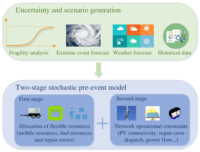
Damage scenarios for extreme weather events are generated based on: (1) identification of extreme weather events, such as flood, hurricane and winter storm; (2) extreme weather event data and metric; (3) fragility model of test systems, which describes the behavior of components under extreme weather events; (4) damage status of components in test system subject to specific extreme weather events. To approximate the impact of extreme weather events to grid infrastructures, damage scenarios can be generated by mapping the weather data set to failure probability of grid infrastructures. Adopted from [17], the failure probability of an overhead line being damaged by hurricane can be expressed as follows:
| (1) |
where is the failure probability of the overhead line with wind speed . is defined as the conditional failure probability of pole at line as a log-normal cumulative distribution function (CDF) of the wind speed , which is expressed in equation (2). and are the number of distribution poles supporting line and the number of conductor wires between two adjacent poles at line , respectively. In equation (3), represents the failure probability of conductor between two poles.
| (2) |
| (3) |
where and are the median capacity and the logarithmic standard deviation of intensity measurement, respectively. represents the direct wind-induced failure probability of conductor and represents the fallen tree-induced failure probability of conductor . is the probability that conductor is underground, which is more invulnerable to extreme weather events. represents the average tree-induced damage probability of overhead conductors. More details of weather forecasting methodologies, line fragility models and scenario generation can be found in [18].
As shown in Figure 1, the proposed SMILP pre-event preparation model has two stages: (i) Flexible resources are allocated in the first-stage, including the optimal number and position of MEGs and MESs, allocation of available fuel to generators, and pre-position of repair crews to depots. (ii) The second-stage optimizes the operation of the distribution system and assign crews to the damaged components. Constraints in the second-stage includes unbalanced optimal power flow constraints, network reconfiguration and isolation constraints, and repair crew scheduling constraints.
2.1 Model Objective Function
The objective function (2.1) is set to minimize operation costs and maximize load served. There are three cost related terms in the objective, cost of fuel , cost of switching operation , and cost of load shedding . The objective is formulated as follows:
| (4) |
where is the probability of occurrence for scenario , is the rate of fuel consumption of a generator, and is the active power output for fuel-based generator at bus , phase , time , and scenario . Binary variable represents the status of each switch, if switch is operated at time on scenario , then . The binary variable represents the status of load at bus , time , and scenario . If the demand () is served, then .
2.2 First-Stage Constraints
The first-stage constraints revolve around pre-allocating four critical resources that will be utilized after an extreme event: (i) MEGs, (ii) MESs, (iii) fuel and (iv) repair crews.
2.2.1 Mobile Resources Allocation Constraints
Mobile resources can be used to restore energy for isolated areas that are not damaged, and to restore critical customers. In addition, fuel management is critical after an extreme event to operate emergency generators. Distributing fuel after an extreme event maybe difficult due to road conditions. As for repair crews, pre-assigning them to different locations provides a faster and more organized response. The constraints for allocating the mobile resources are modeled as follows:
| (5) |
| (6) |
| (7) |
where binary variables and equal 1 if an MEG and MES are allocated to bus , respectively. The set represents the set of candidate buses for MEGs and MESs. Constraints (5) and (6) indicates that the number of installed MEGs and MESs are equal to the number of available devices ( and ). We assume that each bus can only have a limited number of mobile units , which is enforced by (7).
2.2.2 Fuel Resources Allocation Constraints
Define the set , where is the set of buses that have fuel-based emergency generators. The fuel allocated to must be limited to the available amount of fuel. We model the fuel allocation constraints as follows:
| (8) |
| (9) |
Constraint (8) limits the total amount of allocated fuel to the amount of fuel available (), where is the amount of fuel allocated to the generator at bus . Constraint (9) limits the amount of fuel on each site, where is the amount of fuel already present for the generator at bus , and represents the maximum capacity of fuel at bus .
2.2.3 Repair Crew Allocation Constraints
In order to allocate the repair crews, we divide the network into different regions . Each region will be assigned with different crews, who will conduct the repairs in that region. The repair crews are pre-positioned to the regions using constraints (10) and (11), as follows:
| (10) |
| (11) |
where is the number of repair crews in region and is the total number of crews. The number of repair crews is limited in each region, using and , depending on the size and capacity of the staging locations.
2.3 Second-Stage Constraints
In the second-stage of the proposed pre-event preparation model, the constraints of PV systems and repair crew dispatch are mainly discussed. The model also considers unbalanced power flow constraints, voltage constraints and reconfiguration constraints [19, 20].
2.3.1 PV System Constraints
To fully investigate the impact of PV systems on system resilience, three types of PV systems [20] are considered in the second-stage, : (i) Type 1: on-grid (grid-following) PV (), where during an outage, the PV is switched off. (ii) Type 2: hybrid on-grid/off-grid PV + energy storage system (ESS) (), where the PV system operates on-grid in normal conditions, and off-grid during an outage. (iii) Type 3: grid-forming PV + ESS with grid-forming capability (), this system can restore part of the network that is not damaged if the fault is isolated. The output power of the PV systems is determined using the following equations:
| (12) |
| (13) |
| (14) |
| (15) |
The active power output of a PV depends on the rating of the solar cell and the solar irradiance [21]. The generated output power from the PV can be determined in constraints (12) and (13), respectively. The binary variable equals 1 if bus is energized at time and scenario . Using advanced PV smart inverters [22], the PVs can provide reactive power support , which is constrained by the capacity in (14) and (15). During an outage, on-grid PVs are disconnected and the on-site load is not served by the PVs, therefore, constraints (13) and (15) are multiplied by . PV systems of types and can disconnect from the grid and serve the on-site load.
An example network with damaged line is given in Figure 2, where the network is divided into three islands due to the damaged line. In this work, we assume that the network can be restored using the grid-forming sources in . While PV system in types or can connect to the grid only after the PV bus is energized. Island A has a grid-forming generator, therefore, a microgrid is created and the PV system can participate. Island B must be isolated because of the damaged line. Island C does not have any grid-forming generators; hence, it will not be active and the grid-tied PV will be disconnected.

To determine the connection status of the PV systems, we design a virtual network in parallel to the distribution network. The example network shown in Figure 2 is transformed to a virtual network shown in Figure 3.

A virtual network with virtual sources, loads, and flow is built to identify if an island can be energized by grid-forming generators. Each grid-forming generator is replaced by a virtual source with infinite capacity. Other power sources without grid-forming capability (e.g., grid-tied PVs) are removed. The actual loads are replaced by virtual loads with magnitude of 1. The virtual network scheme is modeled using constraints (16)-(20).
| (16) |
| (17) |
| (18) |
| (19) |
| (20) |
A power-balance equation is added for each virtual bus, which means that if the virtual load at a bus is served, then that bus is energized. Therefore, for islands without grid-forming generators, all buses will be de-energized as the virtual loads in the island cannot be served. Constraint (16) is the node balance constraint for the virtual network. Virtual source is connected to buses with power sources that have the capability to restore the system. The variable represents the virtual flow on line and each bus is given a load of 1 that is multiplied by . Therefore, (bus is energized) if the virtual load can be served by a virtual source and 0 (bus is de-energized) otherwise. The virtual flow is limited by (17). The limits are multiplied by the status of the line () so that the virtual flow is 0 if a line is disconnected. The virtual source can be used only if a generator is installed, as enforced by (18). Define as the set of all buses. If bus is de-energized, then the load must be shed (19), unless bus has a local power source with disconnect switch. Constraint (20) is similar to (19) but with the presence of mobile sources.
2.3.2 Repair Crews Constraints
In the second-stage, repair crews are assigned to damaged components that are in the area at which they are positioned. Note that the travel time is neglected in this study, as the travel distances between components in the same area is assumed to be small. An example for crew assignment is given in Figure 4, where two working areas are assigned for the crews. In this example, four damaged lines in Area 1 will be repaired by crews 1-3, while crews 4 and 5 are responsible for the two damaged lines in Area 2. The repair crews constraints are formulated as follows:
| (21) |
| (22) |
| (23) |

Define as a binary variable that equals 1 if line is being repaired at time on scenario , and as the set of damaged lines on scenario . Constraint (21) limits the number of repairs being conducted in each area according to the number of crews available. Constraint (22) defines the repair time for each damaged line. The line status equals 0 until the repair process is conducted for time periods. Based on constraint (23), let , , then . For example, when and , then constraint (23) becomes , therefore, .
2.3.3 Network Operational Constraints
The next set of constraints are related to the operation of distribution systems. We consider unbalanced power flow equations, radiality constraints, fuel consumption, and energy storage constraints. The unbalanced distribution system constraints are given below:
| (24) |
| (25) |
| (26) |
| (27) |
| (28) |
| (29) |
| (30) |
| (31) |
| (32) |
| (33) |
| (34) |
| (35) |
Constraints (2.3.3) and (2.3.3) are the active and reactive nodal power balance constraints, where and are the active and reactive line flows, and and are the power outputs of the generators. The active charging/discharging and reactive power outputs of energy storage systems are denoted by , and . Constraints (26)-(27) represent the active and reactive power limits of the lines, where the limits ( and ) are multiplied by the line status binary variable . Therefore, if a line is disconnected or damaged, power cannot flow through it. Constraints (28)-(29) limit the output of the generators to and . Similarly, we limit the output of the MEGs in (30)-(31) if an MEG is installed ().
Constraints (32) and (33) calculate the voltage difference along line between bus and bus , where is the square of voltage magnitude of bus . We use the big-M method to relax constraints (32) and (33), if lines are damaged or disconnected. and are the unbalanced three-phase resistance matrix and reactance matrix of line , which can be referred to [22]. The vector represents the phases of line . Constraint (34) guarantees that the voltage is limited within a specified region ( and ), and is set to 0 if the bus is in an outage area. Constraint (35) can guarantee the radiality network during the network reconfiguration. In this paper, we assume that all the possible loops can be identified by depth-first search method. The set of loops are given by , and the set of switches in loop is given by . For each fuel-based generator, the total fuel consumption is limited by the available fuel resources in constraint (36), as follows:
| (36) |
Next, we model the operation constraints for ESSs and MESs. The constraints include the change in state of charge (SOC), charging and discharging limits, and reactive power limits. Let be the set of buses with ESSs, and . We can then define the energy storage constraints as follows:
| (37) |
| (38) |
| (39) |
| (40) |
| (41) |
| (42) |
| (43) |
| (44) |
Constraint (37) determines the state of charge of ESSs (). denotes the maximum capacity of the storage system. To ensure safe ESS operation, the SOC and charging () and discharging () power of ESSs are constrained as shown in (38)-(40). Here, , , and define the permissible range of SOC, and maximum charging and discharging power, respectively. In constraints (39)-(40), the binary variable indicates that ESSs cannot charge and discharge at the same time instant. The ESS charging/discharging efficiency are represented by /. The reactive power of ESS, , is kept within maximum limit, , through constraint (41). For MES units, we add constraint (42)-(43) so that if , the output power is 0 at bus . The same method is applied for the reactive power in (44).
3 Solution Algorithm
When the number of scenarios is finite, a two-stage stochastic problem can be modeled as a single-stage large linear programming model, where each constraint in the problem is duplicated for each realization of the random data. For problems where the number of realization is too large or infinite, the Monte Carlo sampling technique can be used to generate a manageable number of scenarios. In this work, we use the scenario decomposing method PH to solve the proposed two-stage stochastic pre-event preparation problem.
3.1 Two-stage Progressive Hedging Algorithm
The proposed two-stage stochastic pre-event preparation problem (2.1)-(44) can be compactly reformulated with an extensive form (EF) as follows:
| (45) |
| (46) |
where and are vectors containing the coefficients associated with the compact first-stage variable and compact second-stage variable in the objective (45), respectively. The constraint (46) represents the subproblem constraints that ensure a feasible solution. The PH algorithm decomposes the extensive form into scenario-based subproblems, by relaxing the non-anticipativity of the first-stage variables. Hence, with the total number of scenarios, the proposed stochastic pre-event preparation problem is decomposed into subproblems. The proposed two-stage PH algorithm is presented in Algorithm 1. Define as iteration number, as a penalty factor and as a termination threshold. The PH algorithm starts by solving the subproblems with individual scenarios. Note that for an individual scenario, the two-stage model is reformulated to a single-level problem. In Step 4, the first-stage solution obtained from Step 2 is aggregated to obtain the expected value . Step 5 calculates the value of the multiplier . In Step 8, the subproblems are solved, where each subproblem is augmented with a linear term proportional to the multiplier and a squared two norm term penalizing the difference of from . Steps 9-10 are similar as Steps 4-5. The algorithm terminates once all first-stage decisions converge to a common .
3.2 Convergence and Solution Validation
As shown in Algorithm 1, the convergence metric of progressive hedging algorithm at each iteration is expressed as the deviation from the mean summed across all first-stage variables and the average value of the first-stage variable as follows:
| (47) |
Numerical results for convergence analysis are given in case study section. In order to test the solution quality based on the limited generated damage scenarios, we follow the suggestion from [20] and apply MRP to test the stability and quality of the candidate solutions, as shown in Algorithm 2. MRP is to repeat the procedure of generating scenarios and solving the proposed model for times and construct the confidence interval (CI) for the optimality gap. The detailed steps in MRP is shown in Algorithm 2, where is the gap estimate and is the sample variance.
4 Case Study
In this section, a large-scale system is used as a test case to verify the scalability and effectiveness of the two-stage stochastic pre-event resource allocation model. This large-scale system consists of 3 existing test systems, EPRI ckt5, ckt7 systems [23], and IEEE 8500 bus system [24], Following the suggestions from [25], the cost parameters in the simulation are , , and . The stochastic models and algorithms are implemented using the PySP package in Pyomo [26]. IBM’s CPLEX 12.6 mixed-integer solver is used to solve all subproblems. The experiments were performed on Iowa State University’s Condo cluster, whose individual blades consist of two 2.6 GHz 8-Core Intel E5-2640 v3 processors and 128 GB of RAM.
4.1 Pre-Event Preparation Results
In this case, we have included 9 depots that are hosting a total of 27 crews, 9 dispatchable DGs, 8 MEGs, 3 MESs, 123 switches, 5 small PVs, 15 large PVs, and 12 ESSs. The 9 DGs are rated at 300 kW and 250 kVAr. The 5 small PVs are rated at 11kW22kW. The 15 large PVs are rated at 500 kW. The 12 ESSs are rated at 500 kW/ 3500 kWh. The pre-event preparation model of the large-scale system is solved in 10.2 hours with 10 damage scenarios. The first-stage decision variables (locations of MEGs, MESs and crews) are shown in Figure 5. 27 crews are allocated to 9 different depots. The value inside the crew depot in Figure 5 represents the number of crews assigned to that depot. Areas with large number of crews indicates that the lines in the area have high damage probabilities.

As discussed in Section 3.2, we use the convergence metric to evaluate the convergence speed of the proposed model. At the same time, we also compare the computational speed with and without a soft-start solution. Soft-start solution means that the previous computed solution in other instance will be used as the starting point. The comparison result is shown in Figure 6. If the convergence metric reaches the convergence threshold 0.01, the algorithm will stop and obtain the optimal solution. The instance with soft-start solution converges at 57 iteration and takes 10.2 hours. The case without soft-start solution converges after 100 iteration and takes 24.3 hours. To test the solution quality with MRP, based on the limited generated damage scenarios, the one-sided CI of the obtained solution is . This small gap indicates that our solution is stable and of high quality.

To evaluate the performance of the developed pre-event preparation model, the model is compared to a base model. The base case is generated by the following steps: (i) one MEG are prepositioned at the substations. (ii) Extra MEG are prepositioned at high-priority loads. (iii) PV and ESS are not considered. (iv) Fuel is allocated to the MEGs such that they can operate for at least 24 hours. (v) Crews are allocated evenly between depots. In this work, we calculate average outage duration by dividing the sum of outage durations for the loads with the number of loads. To compare the performance of the proposed model and the base model, we generate a random scenario and test the response of the system. The generated scenario has 103 damaged lines and they were aggregated to 34 damaged areas in Figure 7. Each circle represents the repair time needed for the specific damaged area considering all the aggregated damaged lines.

The comparison between the base model and the proposed method is shown in Figure. 8. In the base model, the total restored energy is 231,422.38 kWh and the average outage duration is 14.69 hours. In the proposed method, the total restored energy is 291,727.48 kWh and the average outage duration is 11.28 hours. Therefore, approximately 20.67% more loads are served by the proposed method and the outage duration decreased by 30.22%.

4.2 Impacts of Solar PV on System Resilience
To show the advantages of the PV systems, we test the response of the system with the proposed method and different PV penetration levels. As discussed in Section 2.3.1, we consider three types of PV: (i) Type I PV, which represents residential PV panels and the rated capacity is assumed to be 6 kW; (ii) Type II PV, which represents mid-size PV systems and the rated capacity is assumed to be 48 kW; (iii) Type III PV, which represents large utility PV farm and the rated capacity is assumed to be 2000 kW. Based on the number of different types of PVs, we define 6 PV penetration levels as 9%, 27%, 45%, 63%, 81%, and 99%. The number of Type I, II and III PVs for each PV penetration levels is summarized in Table 1. To better collaborate the setting of PV penetration, the number of dispatchable DGs has been changed to 10 and the positions of those DGs have been changed accordingly. The rest of case settings keep the same.
|
|
|
|
|||||||||
|---|---|---|---|---|---|---|---|---|---|---|---|---|
| 9% | 8 | 1 | 1 | |||||||||
| 27% | 24 | 4 | 3 | |||||||||
| 45% | 40 | 7 | 5 | |||||||||
| 63% | 63 | 9 | 7 | |||||||||
| 81% | 72 | 12 | 9 | |||||||||
| 99% | 88 | 15 | 11 |
Based on the results of Figure. 9, it can be observed that different PV penetration levels have different allocation results of the flexible resources, including the positions of MEGs, MESs and number of repair crews.

Figure. 10 shows the percentage of power served during the event, and after the repair process starts. Table 2 and Table 3 compare the amount of load served and average outage duration with different levels of PV penetration.

Based on the results from Figure. 10, Table 2 and Table 3, it can be seen that the penetration of PV contributes to enhancing system resilience. Approximately 31.13% more loads are served compared to the base model when the proposed method with 99% PV penetration is used. Also, the average outage duration decreased by 31.12%. However, compared with the case of 81% PV penetration level, the proposed method with 99% PV penetration does not have significant improvement.
|
|
| ||||||
|---|---|---|---|---|---|---|---|---|
| 0 | 251,210.72 | - | ||||||
| 9% | 318,668.37 | 26.85 | ||||||
| 27% | 335,525.77 | 33.56 | ||||||
| 45% | 336,710.74 | 34.04 | ||||||
| 63% | 344,588.22 | 37.17 | ||||||
| 81% | 360,668.04 | 43.57 | ||||||
| 99% | 364,785.93 | 45.21 |
|
|
| ||||||
|---|---|---|---|---|---|---|---|---|
| 0 | 14.69 | - | ||||||
| 9% | 12.33 | 16.07 | ||||||
| 27% | 11.72 | 20.22 | ||||||
| 45% | 11.65 | 20.69 | ||||||
| 63% | 11.21 | 23.69 | ||||||
| 81% | 10.45 | 28.86 | ||||||
| 99% | 10.12 | 31.11 |
5 Conclusion
In this paper, we develop a two-stage stochastic pre-event resource allocation method for upcoming extreme events, which enables faster and more efficient post-event restoration. The proposed pre-event method leverages the pre-allocation of mobile resources, fuel resources and labor resources. It also facilitates the benefits of distributed PV systems in resilience improvement of distribution grids. According to the case studies, we have the following observations: (i) Compared to the base model without pre-event resource allocation, the proposed pre-event preparation model can serve more loads and reduce the outage duration. (ii) Based on the response of the system with different PV penetration levels, it can be observed that the proposed pre-event preparation model with high PV penetration can further improve system resilience and reduce the outage duration. Therefore, PV systems can play a critical role in improving distribution grid resilience and further promote the renewable energy deployment. (iii) By considering the trade-off between solution accuracy and computation efficiency, the result of MRP indicates that the proposed model’s solutions with a limited number of scenarios can be very stable and of high quality. The scalability of the proposed pre-event preparation model is verified with a large-scale system.
Acknowledgement
This work was supported by the U.S. Department of Energy Wind Energy Technologies Office under Grant DE-EE0008956.
References
- Salman et al. [2015] A. M. Salman, Y. Li, M. G. Stewart, Evaluating system reliability and targeted hardening strategies of power distribution systems subjected to hurricanes, Reliability Engineering & System Safety 144 (2015) 319–333.
- of the President [2020] E. O. of the President, Economic benefits of increasing electric grid resilience to weather outages, Technical Report, White House Tech. Rep., 2020.
- Gholami et al. [2019] A. Gholami, T. Shekari, S. Grijalva, Proactive management of microgrids for resiliency enhancement: An adaptive robust approach, IEEE Trans. Sustain. Energy 10 (2019) 470–480.
- Wang et al. [2017] C. Wang, Y. Hou, F. Qiu, S. Lei, K. Liu, Resilience enhancement with sequentially proactive operation strategies, IEEE Trans. Power Syst. 32 (2017) 2847–2857.
- Panteli et al. [2017] M. Panteli, P. Mancarella, D. N. Trakas, E. Kyriakides, N. D. Hatziargyriou, Metrics and quantification of operational and infrastructure resilience in power systems, IEEE Trans. Power Syst. 32 (2017) 4732–4742.
- Wang et al. [2004] S. Wang, B. R. Sarker, L. Mann, E. Triantaphyllou, Resource planning and a depot location for electric power restoration, Euro. J. Oper. Res. 155 (2004) 22–43.
- Arif et al. [2018] A. Arif, Z. Wang, J. Wang, C. Chen, Power distribution system outage management with co-optimization of repairs, reconfiguration, and DG dispatch, IEEE Trans. Smart Grid 9 (2018) 4109–4118.
- Arif et al. [2020] A. Arif, Z. Wang, C. Chen, B. Chen, A stochastic multi-commodity logistic model for disaster preparation in distribution systems, IEEE Trans. Smart Grid 11 (2020) 565–576.
- Taheri et al. [2019] B. Taheri, A. Safdarian, M. Moeini-Aghtaie, M. Lehtonen, Enhancing resilience level of power distribution systems using proactive operational actions, IEEE Access 7 (2019) 137378–137389.
- Lei et al. [2018] S. Lei, J. Wang, C. Chen, Y. Hou, Mobile emergency generator pre-positioning and real-time allocation for resilient response to natural disasters, IEEE Trans. Smart Grid 9 (2018) 2030–2041.
- Lei et al. [2019] S. Lei, C. Chen, H. Zhou, Y. Hou, Routing and scheduling of mobile power sources for distribution system resilience enhancement, IEEE Trans. Smart Grid 10 (2019) 5650–5662.
- Kim and Dvorkin [2019] J. Kim, Y. Dvorkin, Enhancing distribution system resilience with mobile energy storage and microgrids, IEEE Trans. Smart Grid 10 (2019) 4996–5006.
- Samara et al. [2020] S. Samara, M. F. Shaaban, A. H. Osman, Optimal management of mobile energy generation and storage systems, IEEE Access 8 (2020) 203890–203900.
- Belding et al. [2020] S. Belding, A. Walker, A. Watson, Will solar panels help when the power goes out?, Technical Report, National Renewable Energy Tech. Rep., 2020.
- Rockafellar and Wets [1991] R. T. Rockafellar, R. J.-B. Wets, Scenarios and policy aggregation in optimization under uncertainty, Mathematics of operations research 16 (1991) 119–147.
- Watson and Woodruff [2011] J.-P. Watson, D. L. Woodruff, Progressive hedging innovations for a class of stochastic mixed-integer resource allocation problems, Computational Management Science 8 (2011) 355–370.
- Ma et al. [2018] S. Ma, B. Chen, Z. Wang, Resilience enhancement strategy for distribution systems under extreme weather events, IEEE Trans. Smart Grid 9 (2018) 1442–1451.
- Ma et al. [2019] S. Ma, S. Li, Z. Wang, F. Qiu, Resilience-oriented design of distribution systems, IEEE Trans. Power Syst. 34 (2019) 2880–2891.
- Chen et al. [2018] B. Chen, C. Chen, J. Wang, K. L. Butler-Purry, Sequential service restoration for unbalanced distribution systems and microgrids, IEEE Trans. Power Syst. 33 (2018) 1507–1520.
- Arif et al. [2020] A. Arif, Z. Wang, C. Chen, J. Wang, Repair and resource scheduling in unbalanced distribution systems using neighborhood search, IEEE Trans. Smart Grid 11 (2020) 673–685.
- Melhem et al. [2018] F. Y. Melhem, O. Grunder, Z. Hammoudan, N. Moubayed, Energy management in electrical smart grid environment using robust optimization algorithm, IEEE Trans. Industry Applications 54 (2018) 2714–2726.
- Zhang et al. [2019] Q. Zhang, K. Dehghanpour, Z. Wang, Distributed CVR in unbalanced distribution systems with PV penetration, IEEE Trans. Smart Grid 10 (2019) 5308–5319.
- EPRI [2019] EPRI, OPENDSS test circuits, Apr.2019. URL: https://sourceforge.net/p/electricdss/discussion/beginners.html.
- Arritt and Dugan [2010] R. F. Arritt, R. C. Dugan, The IEEE 8500-node test feeder, in: IEEE PES T&D Conference, 2010, pp. 1–6.
- Ma [2020] S. Ma, Resilience-oriented design and proactive preparedness of electrical distribution system, PhD Thesis (2020).
- Hart et al. [2017] W. E. Hart, C. D. Laird, J.-P. Watson, D. L. Woodruff, G. A. Hackebeil, B. L. Nicholson, J. D. Siirola, Pyomo-optimization modeling in python, volume 67, Springer, 2017.