The Stability of the -family of Peakon Equations
Abstract
In the present work we revisit the -family model of peakon equations, containing as special cases the (Camassa-Holm) and (Degasperis-Procesi) integrable examples. We establish information about the point spectrum of the peakon solutions and notably find that for suitably smooth perturbations there exists point spectrum in the right half plane rendering the peakons unstable for . We explore numerically these ideas in the realm of fixed-point iterations, spectral stability analysis and time-stepping of the model for the different parameter regimes. In particular, we identify exact, stationary (spectrally stable) lefton solutions for , and for , we dynamically identify ramp-cliff solutions as dominant states in this regime. We complement our analysis by examining the breakup of smooth initial data into stable peakons for . While many of the above dynamical features had been explored in earlier studies, in the present work, we supplement them, wherever possible, with spectral stability computations.
1 Introduction
The family of partial differential equations
| (1) |
labeled by the parameter , is distinguished by the fact that it includes two completely integrable equations, namely the Camassa-Holm equation (the case [1, 2]), and the Degasperis-Procesi equation (the case [3, 4]). Each of the two integrable cases has a Lax pair (and is, thus, solvable via the inverse scattering transform), possesses multi-soliton solutions, and a bi-Hamiltonian structure [5, 6, 2, 7]. Furthermore, the cases have been singled out by various tests of integrability: The Wahlquist-Estabrook prolongation method, the Painlevé analysis, symmetry conditions, and a test for asymptotic integrability [3, 8, 9, 10].
The Camassa-Holm equation was originally proposed as a model for shallow water waves [1, 2]. The results of [11, 12] (see Proposition 2 of [11] and Equation (3.8) of [12]) show that, in a model of shallow water, the solution of Eq. (1) corresponds to the horizontal component of velocity evaluated at some specific level in the cases or . However, there is some debate about the precise range of validity of such models [13].
What makes the -family particularly interesting to study from a mathematical physics viewpoint is that it shares the one-peakon solutions
| (2) |
that are admitted by the Camassa-Holm, and the Degasperis-Procesi equations. Indeed, the peakons can solve the following weak formulation of Eq. (1)
| (3) |
where denotes convolution; the fact that is a Green’s function for the operator was used in the reformulation. In effect, Eq. (3) is obtained from Eq. (1) by factoring out the operator .
Moreover, the whole -family possesses -peakon solutions given by
| (4) |
where the positions and amplitudes are the canonically conjugate coordinates and momenta in a finite-dimensional Hamiltonian system. In the cases this Hamiltonian system is completely integrable in the Liouville-Arnold sense [1, 2, 4]. In the general case, the Hamiltonian system does not appear to be integrable [14]. Recently, the -family was generalized to an equation containing two free functions with the property that it also admits multi-peakon solutions written as a linear combination of one-peakons [15].
Another interesting aspect of the -family in the cases is that they admit smooth multi-soliton solutions on a nonzero background [5, 1, 2]. In the limit where the background goes to zero, the -soliton solutions become the -peakons solution as given in Eq. (4). For general , smooth one-solitons on nonzero background are known to exist [16].
The work of [17, 18] presented a numerical study of the solutions of Eq. (1) for different values of . They observed that there are three distinct parameter regimes separated by bifurcations at and , as follows:
- •
Peakon regime: For , arbitrary initial data asymptotically separates out into a number of peakons as .
- •
Ramp-cliff regime: For , solutions behave asymptotically like a combination of a “ramp”-like solution of Burgers equation (proportional to ), together with an exponentially-decaying tail (“cliff”).
- •
Lefton regime: For , arbitrary initial data moves to the left and asymptotically separates out into a number of “leftons” as , which are smooth, exponentially localized, stationary solitary waves.
The behavior observed separately in each of the parameter ranges and can be understood as particular instances of the soliton resolution conjecture [19], a somewhat loosely defined conjecture which states that for suitable dispersive wave equations, solutions with “generic” initial data will decompose into a finite number of solitary waves plus a radiation part which disperses away. The authors of [20] provide a first step towards explaining this phenomenon analytically in the “lefton” regime . Indeed, they show that in this parameter range a single lefton solution is orbitally stable, by applying the approach of Grillakis, Shatah and Strauss in [21]. The main ingredients required for the stability analysis are the Hamiltonian structure and conservation laws for Eq. (1). The -family is known to admit a Hamiltonian structure and two additional conservation laws [22]. The lefton solutions are a critical point for a functional which is combination of the Hamiltonian and a conserved functional.
In this article, our goal is to study the spectral stability of the peakon solutions [cf. Eq. (2)]. In particular, we are interested in the observation made numerically by Holm and Staley in [17, 18] that the peakon solutions become unstable when . To do so, in Section 2, we state the main analytical results concerning the spectrum associated to the eigenvalue problem arising from the linearization of Eq. (3) about the peakon solutions. These analytical results are proven in Section 3. The numerical results on the -family [cf. Eq. (1)] are presented in Section 4. We explore both statically as appropriate, as well as dynamically, each of the classes of solutions therein. We examine their existence over parametric variations of , when possible/relevant (e.g. for the leftons) we consider their stability and we also explore their dynamics (especially for the ramp-cliff waveforms for which we cannot identify a reference frame in which they appear as steady). In Section 5, we state our conclusions and present directions for future study.
2 Main Results
The spectral stability of the peakon solution is explored by first considering Eq. (3) in the co-traveling frame :
Now consider a small perturbation of the peakon of the form
where stands for the eigenvector associated with the eigenvalue . Then, we substitute into Eq. (3) and linearize by keeping only the first-order terms in . This way, we obtain the following eigenvalue problem associated to an integral operator
| (5) |
For our analytical study, we are interested in the spectrum of defined above.
To define an appropriate domain for the operator , we need to consider well-posedness of the -family [cf. Eq. (3)]. The -family is known to be well-posed for initial conditions in , [23, 24, 25, 26, 27, 28, 29]. The peakons in the Camassa-Holm () are proven to be stable in [30] while the ones in the Degasperis-Procesi () in [31]. However, due to the discussion above about well-posedness, the authors of [30] and [31] state that their stability results only apply to initial condition that are in the subsets , , of (for Camassa-Holm) or (for Degasperis-Procesi).
We are thus interested in the orbital stability of the peakon solutions (2) with respect to initial conditions of the form
where is introduced to take into account a drift along the translation invariance symmetry direction. A necessary condition for the initial conditions above to be in , for some is that be in , for all , since itself is in , for all . Thus, at the linear level, we will look for eigenvectors of the form
| (6) |
for , for all . However, is discontinuous and thus not in the domain of as defined in Eq. (5) due to the term . In the next section (see Eq. (22)), we will define an extension of the operator given in Eq. (5) that admits discontinuous functions in its domain. For , we will be interested in eigenfunctions in the set
| (7) |
The extension is not a closed operator on and thus its resolvent set is automatically empty (see for example [32]). However, we show that is closed on the Banach space (see Lemma 3.4), where is the set of bounded functions that are continuous except at the origin, where the functions are allowed to have a finite jump discontinuity (see Eq. (24)). In Section 3, we prove the following theorem about the point spectrum of :
Theorem 2.1.
The second statement within the Theorem 2.1 above provides an explanation for the observation made numerically by Holm and Staley in [17, 18] that the peakon solutions are unstable when . Remark 3.6 illustrates the fact that if the chosen space is made of functions with more regularity than the ones in , the width of the band obtained in the first part of the Theorem 2.1 decreases. Actually, Eq. (31) shows that with enough regularity, the two bands in Theorem 2.1 can be made as close as one wants to each other. A spectrum consisting of a strip about the imaginary axis also occurs in the study of the peaked periodic wave of both versions of the reduced Ostrovsky equations [33]. Although our solutions are not periodic, the nature of the result is similar.
In what follows, we also explore numerically the waveforms of the model for different values of . We identify the leftons as stationary solutions for and illustrate their potential spectral stability. We dynamically examine the ramp-cliff solutions for and show that progressively refined computations (involving more modes) suggest that the ramp-cliff solutions deform into emitting peakons close to (the more refined the computations, the closer to this phenomenology arises). Beyond in line with the theory above, we find that initial data breaks up spontaneously into arrays of peakons that appear to be dynamically robust. A complementary perspective that we provide to avoid issues with the discontinuity of the peakons involves the stability analysis of the solutions of non-vanishing background, as they approach the vanishing background (i.e., peakon) limit.
3 Computation of the point spectrum
In this section, we compute the point spectrum of Eq. (5) for values of such that . The case where can be obtained from the spectrum of the right side of the complex plane by making the observation that if solves the eigenvalue problem of Eq. (5) for a given value of , then solves that same eigenvalue problem with as the corresponding value of .
We first show that the operator defined in Eq. (5) does not have continuous eigenvectors.
Proposition 3.1.
The eigenvalue problem of Eq. (5) does not have solutions in .
Proof.
Consider the problem of Eq. (5) for . We apply the operator to obtain the following differential equation
| (8) |
where we have used the fact that is a Green’s function for the operator . It turns out there are two solutions to Eq. (8) converging as , one as and one as . There is also a solution diverging as . These decay and growth rates are found by solving the constant coefficient asymptotic system obtained by applying the limit to Eq. (8). Actually, Eq. (8) admits the two explicit solutions and .
It should be noted that in Eq. (8) is a regular singular point with exponents , and . A third solution linearly independent that is not singular at can be found if we assume . It can be defined by its series expansion about
| (9) |
where
| (10) |
Upon adding an appropriate multiple of to , the solution converges as and is zero at . Indeed, let be the solution of Eq. (8) defined as
| (11) |
Then is such that and as .
Applying the operator to the eigenvalue problem of Eq. (5) for , one obtains a differential equation with only one converging solution as given by . Hence, to look for a solution to Eq. (5) that is bounded, in the case where , one considers
Since we look for continuous solution, and because , we need to take . The most general ansatz in this case is
| (12) |
with being the Heaviside function.
Lemma 3.2.
If we substitute into Eq. (5), one obtains
| (13) |
Proof.
By substituting into Eq. (5), it is a straightforward computation to find that
| (14) |
When substituting , there are two cases to consider: and . If , we substitute into Eq. (5) and obtain
| (15) |
For , one uses the fact that satisfies (8) itself obtained by the application of the operator on the eigenvalue problem (5), that is
This implies that is a linear combination of and for . Since converges to zero as , we have that
Furthermore, it can be checked that is continuous at due to the fact that is a a continuous function such that . This check is done using the expression obtained below in Eq. (23) for the extension of . The discontinuous part of on the second line of Eq. (23) is zero if . Thus by continuity, with Eq. (15) that and thus
| (16) |
To prove that Eq. (5) does not have continuous solutions, we need to prove that the right-hand-side (RHS) of Eq. (13) cannot be zero for any and . For the RHS of Eq. (13) to be zero, must be zero since the expression it multiplies is discontinuous. The statement of the proposition then stems from the following lemma.
Lemma 3.3.
Assume that has a positive real part. Let be the unique (up to multiplication by a scalar) solution to Eq. (8) such that and as . Then
Proof.
We make the substitution into Eq. (8) to get a second-order equation for since solves Eq. (8). The new equation admits as a solution. We then make the substitution and get a first-order equation for whose solution is
| (17) |
This way, we have that , thus implying
| (18) |
We substitute in the equation above and integrate both sides from to . We integrate by parts the first term of the left-hand-side (LHS), using the fact that , and obtain
Since the sign of never changes by Eq. (17) and as by Eq. (18), we have that never changes sign for and the integrals above are both nonzero. ∎
∎
We now want to consider solutions to the eigenvalue problem of [cf. Eq. (5)] admitting a discontinuity at the origin such as in Eq. (6). To do so, we introduce an extension of as defined in Eq. (5). We first consider in the case , which we denote by :
where we used the fact that . Then, we use integration by parts to eliminate and obtain
| (19) |
where
In the case of , we get
| (20) |
Thus the extension of the operator (from Eq. (5)) reads
which has a larger domain, and if . Indeed, the domain of (from the definition given in Eq. (5)), is restricted to , while the operator (from Eqs. (19) and (20)) admits functions that have a finite-jump discontinuity at . Furthermore, it is straightforward to verify that is in the kernel of , i.e.
| (21) |
We can group terms in Eqs. (19) and (20) as
| (22) |
and rewrite (by applying the derivative operator in Eq. (22)) as
| (23) |
In order to show that is not closable on , it suffices to show that there is a sequence converging to zero, while does not [34, 32]. We choose the sequence of bump functions defined as
Clearly, converges to 0 in , and all the terms in Eq. (22) do also except for the third one since converges to .
In order to define a space on which is closed, we first introduce the following subspace of made of functions that are continuous everywhere except at . More precisely
| (24) |
The set with the norm is a Banach space, since it is isomorphic to the direct sum equipped with the norm .
The operator is defined almost everywhere on , and thus we have the following lemma.
Lemma 3.4.
The operator is closed on .
Proof.
We first consider the operator defined by
| (25) |
We prove that is compact on followed by the use of Theorem 1.11 of [35]11 1 It states that if an operator is closed, then so is any relatively compact perturbation of that operator..
We first prove that each term on the first line of Eq. (23) is compact on by proving they are compact on both and . They are compact on because each term on the first line of Eq. (23) can be written as an integral operator for some kernel . As such, each of those terms defines a Hilbert-Schmidt integral operator, known to be compact (see [36], p. 262). For example, the first term in parentheses in Eq. (23) corresponds to the kernel
| (26) |
To prove the integral terms in Eq. (23) are compact on , we use the Corollary 5.1 of [37], giving the conditions on the kernel of an integral operator for it to be compact on . Those conditions reduce to the following in the case of dimension.
Assume that there is a constant such that for almost all , and . Then the operator is compact if and only if for any there exist and such that for almost all and all we have
| (27) |
and
| (28) |
To check those conditions on the kernel defined in Eq. (26), we compute its norm and find that it is bounded by . We can also compute the integral in Eq. (27) and find that is is bounded by . Finally, the integral in Eq. (28) is found to be bounded by . The conditions of compactness on can also be verified straightforwardly for the two other terms of the first line of Eq. (23). For the second term, we have
The condition on the norm, and conditions (27) and (28) are verified based on the fact that
For the third term in Eq. (23), we have the kernel
where
Since , we only have to verify the conditions for . An integral computation shows that the norm of is bounded by . Furthermore, another integral computation shows that the integral in (27) is bounded by . For the integral in (28), one has to consider several cases depending on the signs of , , and . In each case, one finds that the integral is bounded by an expression that goes to zero as . Note that it would have been sufficient to show that the integral operators on the first line of Eq. (23) are continuous in order to prove the lemma. However, compactness is the stronger property that may be useful in the future to obtain the full spectrum.
We now prove that the remaining term of defined by
is compact on . To prove compactness, we need to take a bounded sequence of and prove that has a Cauchy subsequence. The boundedness of on implies the boundedness of , with . Thus, the sequence contains a Cauchy subsequence . With the norm we have
and with the norm
Thus, the sequence is a Cauchy subsequence of on both and . We conclude that is compact on .
It now suffices to prove that defined in Eq. (25) is closed. Assume we have a converging sequence in the domain of , such that also is converging. We need to show that . The convergence of the term to in is immediate. For the term , the convergence of to implies the of to . Furthermore, since itself is convergent in , it converges to , by definition of convergence on . The convergence of the term in the sup norm to follows from the fact that converges in both and to the same function, by the definition of the norm on as being the maximum of the two norms. ∎
We are now ready to prove Theorem 2.1.
Proof.
We first compute the point spectrum of associated with the eigenvalue problem of Eq. (22). The most general candidate for a discontinuous solution at is given by Eq. (12). Without loss of generality, we choose
Hence, the most general ansatz for a solution in in this case is
where we used the fact that . Computing , using Eqs. (13) and (21), we find
Thus, is a solution given that and is chosen such that . From the expansions given in Eq. (9), if we add the restriction that be in , we have that
| (29) |
i.e. any satisfying is in the point spectrum.
The following lemma proves the second part of Theorem 2.1.
Lemma 3.5.
Proof.
Because the series expansion of Eq. (9) admits a different form for and , we treat the two cases separately starting with . In view of the definition of from Eqs. (9) and (11), if we require to be in , it implies that . We write as . Because , we have that is in . It thus suffices to show that the function
| (30) |
is in for all if only if . As an example, if we use in Eq. (30), then the Fourier transform of is given by
Recall that the condition for to be in is that be in [38]. This condition is satisfied if and only if . The same condition on is obtained if we use such that and thus it is clear from given by Eq. (30) that it will be in for all if and only if . It can also be checked directly by the following expression giving the Fourier transform of [cf. Eq. (30)] for general values of
where is the Gamma function. As per the case for , from the second line of Eq. (9), we consider the function
which can be verified to be in for all by the expression of its Fourier transform:
where is Euler’s constant. ∎
∎
Remark 3.6.
In Theorem 2.1, we use the space (with defined in (24)). If more regularity is required by using the space
instead, one finds the point spectrum in the first part of Theorem 2.1 to be . Indeed, the proof of Theorem 2.1 goes through with the modification that the condition (instead of specified in Eq. (29)) must be satisfied in order for to be in . The closure of holds because, for any interval , for some constant . Furthermore, if is replaced by , , in the definition of above, then the condition on becomes . This follows from the Fourier transform computation done in the proof of Lemma 3.5 and from Lemma 5.2 of [38] giving a criterion for a function to be in a fractional Sobolev space on a subset of . The band specified in the first part of Theorem 2.1 is then found to be
| (31) |
which limits to the band specified in the second part of Theorem 2.1 as .
4 Numerical Results
In this section, we present numerical results concerning the existence and spectral stability of standing and traveling wave solutions to the -family of equations, i.e., Eq. (1). The discussion that follows next is complemented by systematically presenting results on spatio-temporal evolution of generic (Gaussian) and peakon initial data.
4.1 Standing and traveling waves
First, we shall be interested in the “lefton” solutions. A single lefton is a stationary solution of Eq. (1) given by the explicit formula [22]
| (32) |
where and are its amplitude and center, respectively. For a given , this is a 2-parameter family of solutions, given the arbitrary choice and . The form of Eq. (32) suggests that leftons exist only for the parameter regime . This is confirmed numerically by parameter continuation in . We start with a lefton solution given by Eq. (32) with and , normalized so that . We then increase using a secant-based predictor-corrector parameter continuation algorithm in Matlab. So that a single member of the 2-parameter family is selected, we add the constraints that is an even function and that . In all cases, the parameter continuation stops just before is reached. Since the width of the lefton solution [cf. Eq. (32)] increases as approaches , the exact stopping point depends on the domain size used for continuation, as well as the discretization of the problem (e.g. number of grid points used) and the continuation step size.
We investigate the spectral stability of a lefton solution of the -family as written in Eq. (1). We linearize the -family about and obtain the following eigenvalue problem
| (33) |
where the prime denotes derivative with respect to . We rearrange Eq. (33) to get , where is the linear operator
We can verify directly that , which results from translation invariance of the system. In addition, when , . To find the spectrum, we again use Fourier spectral differentiation matrices for the differential operators and compute the eigenvalues using the built-in eigenvalue solver eig in MATLAB. Figure 1 shows the computed spectrum for a lefton solution with parameter and amplitude ( for all leftons). The maximum real part of the spectrum is of order , suggesting that the spectrum is purely imaginary. In addition, we verify numerically that and . We expect that the additional degree of freedom in in Eq. (32) will generate an eigenfunction in the kernel of , and we can verify numerically that . The same spectral results are obtained for a wide range of and .

For the peakon solutions, which are traveling waves, this method of computing the spectrum does not work since the peakon is not differentiable at its center. As an alternative, we will compute the spectrum of the family of smooth solitary waves on a nonzero background [16], which are solutions to the equation
| (34) |
obtained by integrating the co-traveling frame ODE obtained from Eq. (1). The limit of these smooth solitons, which we compute numerically by parameter continuation in (Figure 2, left panel), is the peakon solution.


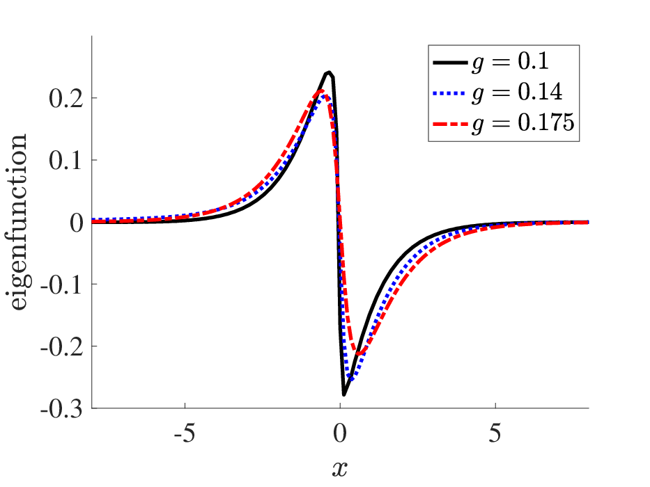
Using the same techniques as above, we can numerically compute the spectrum of these smooth solitons. For , the maximum real part of the spectrum is of order for sufficiently large (Figure 2, bottom left), which suggests that the spectrum is purely imaginary for that parameter regime. When decreases below a threshold value, numerical spectral computation suggests the presence of an eigenvalue with positive real part. This threshold, however, is lower as the number of Fourier modes in the discretization is increased. Furthermore, the eigenfunction associated with this eigenvalue resembles the derivative of the smooth soliton (Figure 2, bottom right), and becomes increasingly singular as decreases. Since the derivative is an eigenfunction with eigenvalue due to translation invariance, this positive real eigenvalue is most likely an artifact resulting from the fact that the solution we are linearizing around becomes increasingly non-smooth as decreases, and this occurs sooner for coarser discretizations. Similar results are obtained for values of between and . Thus, we conclude that for sufficiently large (i.e. ; cf. Fig. 2), the solutions of [16] are spectrally stable; yet, as approaches , we are no longer able to provide definitive spectral conclusions for the stability of the non-smooth peakon solutions, although the above interpretation of our spectral computations (corroborated by dynamical simulations given below) is suggestive of their robustness.
4.2 Numerical timestepping
We now turn our focus to spatio-temporal dynamics of the -family of peakon equations Eq. (1). For our subsequent analysis, we will consider Gaussian initial data of the form of
| (35) |
where and correspond to the width and center of the Gaussian pulse, respectively. The previous works of [17, 18, 39] considered the so-called -formulation
| (36) |
which we adopt from now on, and the numerical scheme we employed in this work is discussed next. We advance Eq. (36) forward in time with the initial data of Eq. (35) by using Fourier spectral collocation for the spatial discretization supplemented by periodic boundary conditions on , and the Runge-Kutta-Fehlberg (RKF45) for the time marching. The latter is a predictor-corrector method (with time step-size adaptation) where we used strict (absolute and relative) tolerances of per time step. Then, at each time step, the field is obtained from by inverting the Helmholtz operator in Fourier space. We should mention in passing that the time integration is performed in Fourier space as well. We remove the aliasing errors by employing the so-called -rule in order to ensure that the high wavenumber Fourier coefficients are well decayed (see, e.g., Ref. [40]). However, we do not employ artificial viscosity as opposed to the works of [17, 18, 39]. This way, it is expected that the numerical results reported herein are close representations of the original physical system.
A series of benchmarks of the numerical scheme is discussed in the Appendix A. In particular, using the initial data of Eq. (35), selected cases of spatio-temporal dynamics in are presented giving rise to peakons, leftons as well as ramp-cliffs, and the results discussed therein are connected with the current literature. For example (see also Figs. 7-9), when , we observe the emergence of solitary pulses from Gaussian initial data [cf. Eq. (35)] that move to the left, gradually asymptoting to a steady-state solution, i.e., leftons [cf. Eq. (32)]. It should be noted in passing that the number of leftons depends on how close or far away the selected value of is from , e.g., we observed the emergence of three and two leftons for and , respectively (see the Appendix A for a detailed discussion on leftons).


We now turn our focus on the ramp-cliff regime corresponding to the case when . In the Appendix A, we present 4 cases of ramp-cliffs where the latter travel faster for gradually increasing values of . We can clearly observe the formation of these patterns and the self-similar expansion of their rear tails, while at the same time their front part steepens. It is worth noting here that we are not aware of a frame where such solutions can be considered as steady. However, we report at this point an artifact that was observed in our numerical simulations with collocation points and interval of time of integration . One would expect the emergence of ramp-cliffs propagating to the right of the computational domain. Nevertheless, for we noticed that peakons were emitted from the ramp-cliffs, with the former emerging as robust traveling waves. We investigated this byproduct of the numerical scheme by considering the implications of Theorem 3 in [20]. In particular, it can be shown that if , then , holds which in fact is the case as per the Gaussian initial data employed in this work.


Upon a careful inspection of the temporal evolution of the variable , we noticed that it becomes negative past a time , thus suggesting that one cannot continue the temporal integration beyond that time (due to the numerical scheme violating a theoretically established constraint). Moreover, we performed a spatial grid refinement by increasing the number of collocation points to in order to investigate further the dependence of on . We still observed the emergence of such “spurious” peakons but their appearance was delayed in time. This finding is somewhat expected: in this computation, we keep our spatial domain fixed during the spatial grid refinement which implies that the wavenumbers are still multiples of . Thus, when the number of collocation points is increased, the numerical scheme resolves progressively better the large wavenumbers which, in turn, results in the time delay of the emergence of those “spurious” peakons. It is expected that if we increase the number of nodes to, e.g., , this artifact will gradually disappear. As case examples of ramp-cliffs (in addition to the ones shown in Fig. 10 in Appendix A), we demonstrate two cases with and in Fig. 3 where we stopped the integrator at (past that time, we observed the non-positivity of the variable).
We now investigate the peakon regime of the -family, i.e.,when . In particular, Fig. 4 presents selective cases of numerical simulations based on Gaussian initial data with and , and Fourier modes. The top left and right panels correspond to the cases with and (CH) whereas the bottom left and right to values of of and (DP), respectively. The emergence of sharply peaked waves can be discerned from these panels where the initial Gaussian pulse breaks into peakons as time progresses. Furthermore, the time when the first peakon emerges in the simulations depends on the value of , that is, its emergence is “delayed” when is close to . However, when the value is further away from that limit, the first peakon emerges at earlier times together with secondary peakons of smaller amplitude traveling across the computational grid. It should be noted also that the first peakon (having actually the largest amplitude) travels in the computational grid and undergoes nearly elastic collisions with other peakons of smaller amplitude. Such phenomenology is interesting in its own right and deserves further study, however it is beyond the scope of the present work.
We finally focus on Theorem 2.1 (see Section 2) which suggests that the point spectrum contains positive eigenvalues for , that is, the peakons are orbitally unstable for . We explore this theoretical finding numerically by considering a peakon centered at with speed (or amplitude) , and collocation points. The left and right panels of the top row of Figure 5 present our numerical results for values of of (left panel) and (right panel), respectively. It can be discerned from both panels that the peakons are orbitally unstable. The amplitude of the initial profile () gradually increases over time eventually leading to a collapse of the waveform (in particular, past for the spatial discretization employed herein).
On the other hand, i.e., when , we expect peakons to be orbitally stable. Indeed, this is the case as is shown in the middle and bottom panels of Fig. 5. In particular, the middle and bottom panels showcase profiles of peakons at and (terminal time of integration) for and , respectively (the same initial condition was used in both cases as in the top row of Fig. 5). It can be discerned from both panels that peakons appear to be robust over the time integration. However, a couple of remarks are in order at this point and in line with the middle and bottom panels of Fig. 5. We observe a small in-amplitude yet stationary localized error at the vicinity of the center () of the initially placed peakon. It has been argued in [41] that when non-smooth initial data are considered in an evolution numerical experiment (such as peakons in the -family), localized errors are expected to be formed in the vicinity of initially that remain stationary in time. This is the case in both panels of Fig. 5 and it is expected that this error gradually diminishes with grid refinement (see [41]). However, this error results in a slightly larger amplitude (and thus speed) of the pertinent peakon waveform but after a “transient” period of time it remains constant over the time evolution, as this can be seen in the insets of the panels. Indicatively, the location of the peakon after time units in the bottom panel (i.e., for ) is found to be at whereas the theoretical expectation is , thus suggesting a (relative) error of . Despite this artifact, peakons for appear to be highly robust and these findings are in accordance with Theorem 2.1.


5 Conclusions and Future Directions
In the present work we have identified the solutions of the -family of peakon equations. We have provided some analytical insight on the spectral problem, identifying the instability of the peakon waveforms via the consideration of their point spectrum. Indeed, we have indicated that the latter contains eigenvalues with a positive real part. Our analytical insights have been corroborated by a diverse array of numerical computations. For structures that we could identify as steady, either in the original frame or in a co-traveling frame, we attempted to offer a complementary spectral picture. This was done in the case of the leftons for which are stationary and were found to potentially be stable in this regime. On the other hand, in the regime , we could only perform dynamical simulations which illustrated the transient emergence and tendency towards breaking of ramp-cliff waveforms. The resulting formation of peakon structures (as ) was identified as a feature that disappears as the high wavenumbers become better resolved. However, the peakon structures become indeed dominant for where they spontaneously arise from smooth initial conditions and robustly persist for different values of , for integrable and non-integrable cases alike. Suggestive, although not definitive, towards their stability is the picture identified spectrally for the solutions on a finite background, tending towards these peakons as the background parameter tends to .
While we believe that this study addresses some of the pending questions on this class of systems admittedly many more questions remain open and are worthwhile to explore in future studies. Is there a meaningful (and consistent with our theoretical analysis) way in which the peakon spectral analysis can be numerically performed? Is there a frame (possibly a self-similarly evolving one) where the ramp-cliff structures can be considered as steady and thus be spectrally analyzed? Are there higher-dimensional analogues of these different structures and, if so, which of the above properties persist or disappear even in the two-spatial-dimension case? These are only some among the numerous open questions. Work in these is currently underway and will be reported in future publications.
Acknowledgments
PGK acknowledges support from the U.S. National Science Foundation under Grants no. PHY-1602994 and DMS-1809074 (PGK). EGC is indebted to Hans Johnston (UMass) for endless support, discussions and guidance throughout this work. He thanks Darryl Holm (Imperial College) for pointing out Ref. [39] and express his gratitude to James (Mac) Hyman (Tulane University) for fruitful discussions during his visit at Los Alamos National Laboratory in 2019. He also express his gratitude to Chi-Wang Shu (Brown University) for discussions about discontinuous Galerkin methods. SL acknowledges a Collaboration Grants for Mathematicians from the Simons Foundation (award # 420847). SL also acknowledges discussions with Andrew Hone (University of Kent) and Simon Eveson (University of York).
Appendix A Spatio-temporal dynamics: From peakons to Leftons and Ramp-Cliffs
We test our numerical scheme by re-producing a subset of the results of Refs. [4] and [17]. In particular, the left () and right () panels of Fig. 6 correspond to the spatio-temporal evolution of by using Gaussian initial data [cf. Eq. (35)] with and , and and respectively. Those results compare well with Figs 1 and 2 of Refs. [17] and [4], respectively.


Next, we focus on the regime . In particular, Figs. 7-9 highlight numerical results on the lefton regime [cf. Eq. (32)] by considering various values of (with Fourier modes). In particular, Fig. 7 presents the spatio-temporal evolution of for the cases with (top left panel), (top right panel), (bottom left panel), and (bottom right panel), respectively, when Gaussian initial data are employed with and . The emergence of leftons is clearly evident in all those panels and we notice the appearance of more leftons when is larger in its absolute value (notice the appearance of four leftons in the top left and right panels whereas the bottom left and right ones contain three and two, respectively). We further investigated the emergence of leftons by considering different values of the Gaussian’s width and center. Specifically, Fig. 8 presents results with (and ) where the number of leftons decreases as approaches .
Fig. 9 compares the numerically obtained (stationary) solution of the top right panel of Fig. 8 with Eq. (32). It should be noted that this result is the analogue of Fig. 6 in [17]. In the present case (with ), three leftons appear at the terminal time of the evolution () whose locations and amplitudes are computed. Then, those values are plugged into Eq. (32) and are plotted with stars, crosses and plus signs in Fig. 9. A perfect match can be clearly discerned, thus suggesting the accuracy and high-fidelity of the numerical scheme employed in this work.


Next, we focus on the regime in which ramp-cliff solutions were suggested to be observed from Gaussian initial data. Fig. 10 corresponds to numerical results with and by employing Fourier modes. In particular, the top left and right panels correspond to the spatio-temporal evolution of with (i.e., at the bifurcation point) and , whereas the bottom left and right ones to and , respectively. From the top left panel of Fig. 10 (), it can be discerned that the Gaussian pulse becomes slightly wider but represents a nearly stationary solution (see, for example, Fig. 5 of [18]). On the other hand, the top right, bottom left and right panels corresponding to , and , respectively, showcase examples of ramp-cliff solutions. It should be noted that their amplitude decreases over the time evolution although their velocity increases with .
References
- [1] R. Camassa and D.D. Holm, Phys. Rev. Lett. 71 (1993) 1661-4.
- [2] R. Camassa, D.D. Holm and J.M. Hyman, Adv. Appl. Mech. 31 (1994) 1-33.
- [3] A. Degasperis and M. Procesi. Symmetry and Perturbation Theory, World Scientific (1999) 23-37.
- [4] A. Degasperis, D.D. Holm and A.N.W. Hone, Theor. and Math. Phys. 133 (2002) 1461–72.
- [5] Y. Matsuno, Inverse Problems 21 (2005) 2085.
- [6] A.N.W. Hone, J. Phys. A 32 (1999) L307-L314.
- [7] B. Fuchssteiner and A.S. Fokas, Physica D 4 (1981) 47-66.
- [8] A.N.W. Hone and J.P. Wang, Inverse Problems 19 (2003) 129-145.
- [9] A.V. Mikhailov and V.S. Novikov. J. Phys. A 35 (2002) 4775-4790.
- [10] A.N.W. Hone, Integrability, ed. A.V. Mikhailov, Lect. Notes Phys. 767, Springer, Berlin, Heidelberg (2009) 245-277.
- [11] A. Constantin and D. Lannes, Arch. Rational Mech. Anal. 192 (2009) 165-186.
- [12] R.I. Ivanov, Phil. Trans. R. Soc. A 365 (2007) 2267-2280.
- [13] R. Bhatt and A.V. Mikhailov, On the inconsistency of the Camassa-Holm equation with the shallow water theory. arxiv:1010.1932v1
- [14] D.D. Holm and A.N.W. Hone, J. Nonlin. Math. Phys. 12, Supplement 1 (2005) 380-94.
- [15] S.C. Anco and E. Recio, J. Phys. A 52 (2019) 125203.
- [16] B. Guo and Z. Liu, Chaos, Solitons & Fractals 23 (2005) 1451-1463.
- [17] D.D. Holm and M. F. Staley, Phys. Lett. A 308 (2003) 437-444.
- [18] D.D. Holm and M.F. Staley, SIAM J. Appl. Dyn. Syst. 2 (2003) 323-380.
- [19] T. Tao. Bull. Amer. Math. Soc. 46 (2009) 1-33.
- [20] A.N.W. Hone and S. Lafortune, Physica D 269 (2014) 28-36.
- [21] M. Grillakis, J. Shatah and W. Strauss, J. Functional Analysis 74 (1987) 160-197.
- [22] A. Degasperis, D.D. Holm and A.N.W. Hone, Proceedings of the Workshop: Nonlinear Physics: Theory and Experiment. II, World Scientific (2002) 37-43.
- [23] G. Gui, Y. Liu, and L. Tian, Indiana University Mathematics Journal 57 (2008) 1209-1234.
- [24] Y. Zhou, Math. Nachr. 278 (2005) 1726-1739.
- [25] Y. Liu and Z. Yin, Comm. Math. Phys. 267 (2006) 801-820.
- [26] J. Escher and Z. Yin, Journal für die reine und angewandte Mathematik (Crelles Journal) 624 (2008) 51-80.
- [27] K. Grayshan, Differential and Integral Equations 25, (2012) 1-20.
- [28] Y.A. Li and P. J. Olver, J. Diff. Eqs. 162 (2000) 27-63.
- [29] G. Rodríguez-Blanco, Nonlinear Analysis 46 (2001) 309-327.
- [30] A. Constantin and W. Strauss, Comm. Pure Appl. Math. 53 (2000) 603–610.
- [31] Z. Lin and Y. Liu, Comm. Pure and Appl. Math. 62 (2009) 125-146.
- [32] K. Schmüdgen, Unbounded self-adjoint operators on Hilbert space Graduate Texts in Mathematics Vol. 265. Springer-Verlag (2012).
- [33] A. Geyer and D. Pelinovsky, Proceedings of the American Mathematical Society 148 (2020) 5109-5125.
- [34] D. E. Edmunds and W. D. Evans, Spectral theory and differential operators, Oxford University Press (2018).
- [35] T. Kato, Perturbation theory for linear operators, Vol. 132, Springer Science & Business Media (2013).
- [36] M. Renardy and R. C. Rogers, An Introduction to Partial Differential Equations, Texts in Applied Mathematics, Springer-Verlag, 2nd edition (2004).
- [37] S. P. Eveson, Proceedings of the American Mathematical Society 123 (1995) 3709-3716.
- [38] E. Di Nezza, G. Palatucci, and E. Valdinoci, Bulletin des Sciences Mathématiques 136 (2012) 521-573.
- [39] O.B. Fringer and D.D. Holm, Physica D: Nonlinear Phenomena 150 (2001) 237-263.
- [40] J. Boyd, Chebyshev & Fourier Spectral Methods: Second Revised Edition, Dover Books on Mathematics (2001).
- [41] D.C. Antonopoulos, V.A. Dougalis and D.E. Mitsotakis, Numerische Mathematik 143 (2019) 833-862.