Dissecting a resonance wedge on
Heteroclinic bifurcationsThanks: AR was partially supported by CMUP (UID/MAT/00144/2019), which is funded by FCT with national (MCTES) and European structural funds through the programs FEDER, under the partnership agreement PT2020. AR also acknowledges financial support from Program INVESTIGADOR FCT (IF/00107/2015).

While some progress has been made, both numerically and analytically, the number of explicit configurations whose flows have an invariant torus and for which the Torus-Breakdown description is available, has remained small.

By studying unfoldings of a Bykov attractor, we are able to delineate the ways in which the first return map to a cross section can make the transition from a single rotation number to an interval of rotation numbers¹¹ 1 The existence of rotational horseshoes, described in Appendix A.8, is responsible for the existence of an interval of rotation number – see [45]. . As a continuation of the project started in [52], we will prove analytically that a sequence of discrete-time Bogdanov-Takens bifurcations organise the dynamics that appear in the unfolding. Besides, within the Arnold wedge, we numerically find surfaces corresponding to the following bifurcations: Hopf, period-doubling and the transition node $\mapsto$ focus. Our results agree well with the literature about heteroclinic bifurcations, Arnold tongues and the scenarios described in [9, 10, 47].

Our object of study is not “just another dynamical system”, but representative for the case of 3-dimensional dissipative flows admitting 2-dimensional connections that are pulled apart. In similar models, the corresponding phenomenology should contain no further secrets.

Our study allows us to understand the bifurcations from an invariant torus to strange attractors that appear in Ruelle and Takens [53] and Langford [40] (see also §6.2 of [20]). In the context of turbulent flows, the author of [40] studied a two-parameter unfolding a Hopf-zero singularity and proved that axisymmetric perturbations generate an invariant torus. By slightly breaking the symmetry, Langford prove that the flow becomes more and more turbulent with fractal basins of attraction as a consequence of the emergence strange attractors. The bifurcations described in our paper have similarities with those described in [54] in the context of a low-order atmospheric circulation model.

In Section 2, we describe precisely our object of study and we review the literature related to it. In Section 3 we state the main results of the article. The coordinates and other notation used in the rest of the article are presented in Section 4 to prove the main results of the manuscript in Section 5.

We refine the structure of Arnold tongues which appear in the context of heteroclinic bifurcations on Section 6. In Section 7, we briefly illustrate our theoretical results with an example explored in [21]. Symmetry-breaking effects will be described.

We finish the article with a discussion in Section 8 about the consequences of our findings. Dynamics similar to what we described is expected to occur near periodically forced attracting heteroclinic cycles. For reader’s convenience, we have compiled at the end of the article (Appendix A) a list of basic definitions.

For $\varepsilon>0$ small, consider the 3-parameter family of $C^{3}$–smooth differential equations

where ${\mathbb{S}}^{3}$ represents the unit three-sphere, endowed with the usual topology. Let us denote by $\varphi_{(A,\lambda,\omega)}(t,x)$, $t\in{\mathbb{R}}$, the flow associated to (2.1) satisfying the following properties for $A=\lambda=0$ and $\omega\in{\mathbb{R}}^{+}$:

1. (P1)

   There are two different equilibria, say $O_{1}$ and $O_{2}$.

2. (P2)

   The eigenvalues of $Df_{X}$ are:

   1. (P2a)

      $E_{1}$ and $-C_{1}\pm\omega i$ where $C_{1},E_{1}>0$, for $X=O_{1}$;

   2. (P2b)

      $-C_{2}$ and $E_{2}\pm\omega i$ where $C_{2},E_{2}>0$, for $X=O_{2}$.

For $W\subseteq{\mathbb{S}}^{3}$, denoting by $\overline{W}$ the closure of $W$, we also assume that:

1. (P3)

   The manifolds $\overline{W^{u}(O_{2})}$ and $\overline{W^{s}(O_{1})}$ coincide and the set $\overline{W^{u}(O_{2})\cap W^{s}(O_{1})}$ consists of a 2-dimensional sphere (${W^{u}(O_{2})\cap W^{s}(O_{1})}$ is called the $2D$-connection).

and

1. (P4)

   There are two trajectories, say $\gamma_{1},\gamma_{2}$, contained in $W^{u}(O_{1})\cap W^{s}(O_{2})$, each one in each connected component of ${\mathbb{S}}^{3}\backslash\overline{W^{u}(O_{2})}$ ($\gamma_{1},\gamma_{2}$ are called the $1D$-connections).

The equilibria $O_{1}$ and $O_{2}$, the $2D$-connection referred in (P3) and the two trajectories $\gamma_{1},\gamma_{2}$ of (P4) build a heteroclinic network, that we denote by $\Gamma$. This network, illustrated in Figure 1, has two cycles. Assuming that the set of eigenvalues of $Df_{O_{1}}$ and $Df_{O_{2}}$ satisfy

1. (P5)

   $\displaystyle\frac{C_{1}C_{2}}{E_{1}E_{2}}\gtrsim 1$

There are two possibilities for the geometry of the flow around the saddle-foci of $\Gamma$, depending on the direction the trajectories turn around the $1D$-connections. This is related to the topological concept of chirality introduced in [37].

Let $V_{1}$ and $V_{2}$ be small disjoint neighborhoods of $O_{1}$ and $O_{2}$ with boundaries $\partial V_{1}$ and $\partial V_{2}$, respectively. These neighborhoods will be precisely constructed in Section 4. Trajectories starting at $\partial V_{1}\backslash W^{s}(O_{1})$ near $W^{s}(O_{1})$ go into the interior of $V_{1}$ in positive time, then follow one of the solutions in $[O_{1}\rightarrow O_{2}]$, go inside $V_{2}$, come out at $\partial V_{2}$ and then return to $\partial V_{1}$ (see Figure 2). This trajectory is not closed since $\Gamma$ is attracting.

Let $\mathcal{Q}$ be a piece of trajectory like this from $\partial V_{1}$ to $\partial V_{1}$. Within $\partial V_{1}\backslash W^{s}(O_{1})$, join its starting point to its end point by a segment as in Figure 2, forming a closed curve, which we call the loop of $\mathcal{Q}$. By construction, the loop of $\mathcal{Q}$ and $\Gamma$ are disjoint closed sets.

The next hypothesis may be written as:

1. (P6)

   The saddle-foci $O_{1}$ and $O_{2}$ have the same chirality.

For $r\geq 3$, denote by $\mathfrak{X}^{r}({\mathbb{S}}^{3})$, the set of 3-parameter family of $C^{3}$–vector fields on ${\mathbb{S}}^{3}$ satisfying Properties (P1)–(P6), endowed with the $C^{r}$–topology.

Concerning the effect of $A$, $\lambda$ and $\omega$ on the dynamics of (2.1), we assume that:

1. (P7)

   For $A>\lambda\geq 0$ and $\omega\in{\mathbb{R}}^{+}$, the two trajectories within $W^{u}(O_{1})\cap W^{s}(O_{2})$ persist.

By the Kupka-Smale Theorem, generically the invariant 2-dimensional manifolds $W^{u}(O_{2})$ and $W^{s}(O_{1})$ are transverse (either intersecting or not):

1. (P8a)

   For $A,\lambda\geq 0$ and $\omega\in{\mathbb{R}}^{+}$, the manifolds $W^{u}(O_{2})$ and $W^{s}(O_{1})$ intersect transversely.

2. (P8b)

   For $A,\lambda\geq 0$ and $\omega\in{\mathbb{R}}^{+}$, the manifolds $W^{u}(O_{2})$ and $W^{s}(O_{1})$ do not intersect.

and

1. (P9)

   Up to high order terms in $x,y$, the transitions along the connections $[O_{1}\rightarrow O_{2}]$ and $[O_{2}\rightarrow O_{1}]$ are given, in the local coordinates that will be defined in Section 4, by the Identity map and by

   $$(x,y)\mapsto(x,y+A+\lambda\Phi(x))$$

   respectively, where $\Phi:{\mathbb{S}}^{1}\rightarrow{\mathbb{S}}^{1}$ is a Morse function with at least two non-degenerate critical points (${\mathbb{S}}^{1}={\mathbb{R}}\pmod{2\pi}$). This assumption will be clearer later.

Once for all, we define the following notation that will be used throughout the present manuscript:

We discuss the Hypotheses (P1)–(P9), stressing that they are natural in several settings. An illustrative scheme of the Hypotheses has been summarized in Table 1 of [52].

In this section, we give an overview of results for the class of vector fields satisfying either (P1)–(P8a)–(P9) or (P1)–(P8b)–(P9).

In order to describe the dynamics around the cycles of $\Gamma$, we use the local coordinates near the equilibria $O_{1}$ and $O_{2}$ introduced in [44] (cf. [38, 52]). In these coordinates, we use cylindrical neighborhoods $V_{1}$ and $V_{2}$ in ${{\mathbb{R}}}^{3}$ of $O_{1}$ and $O_{2}$, respectively, of radius $\rho=\tilde{\varepsilon}>0$ and height $z=2\tilde{\varepsilon}$. After a linear rescaling, we assume $\tilde{\varepsilon}=1$.

The boundaries of $V_{1}$ and $V_{2}$ consist of three components: the cylinder wall parametrised by $x\in{\mathbb{R}}\pmod{2\pi}$ and $|y|\leq 1$ with the cover

and two discs, the top and bottom of the cylinder. We consider polar coverings of these disks

where $0\leq r\leq 1$ and $\varphi\in{\mathbb{R}}\pmod{2\pi}$. In $V_{1}$, we use the notation:

• •

  ${\text{In}}(O_{1})$, the cylinder wall of $V_{1}$, consists of points that go inside $V_{1}$ in positive time;
  

• •

  ${\text{Out}}(O_{1})$, the top and bottom of $V_{1}$, consists of points that go outside $V_{1}$ in positive time.
  

We denote by ${\text{In}}^{+}(O_{1})$ the upper part of the cylinder, parametrised by $(x,y)$, $y\in\,]\,0,1]$ and by ${\text{In}}^{-}(O_{1})$ its lower part. The local stable manifold of $O_{1}$, $W^{s}_{\text{loc}}(O_{1})$, corresponds to the circle parametrised by $y=0$. The cross-sections around $O_{2}$ are dual of the previous sections. The set $W^{s}_{\text{loc}}(O_{2})$ corresponds to the intersection of the $z$-axis with the top and bottom of $V_{2}$; these two intersection points will be the origin of its coordinates. The set $W^{u}_{\text{loc}}(O_{2})$ is defined by $y=0$ and:

• •

  ${\text{In}}(O_{2})$, the top and bottom of $V_{2}$, consists of points that go inside $V_{2}$ in positive time;
  

• •

  ${\text{Out}}(O_{2})$, the cylinder wall of $V_{2}$, consists of points that go outside $V_{2}$ in positive time, with ${\text{Out}}^{+}(O_{2})$ denoting its upper part, parametrised by $(x,y)$, $y\in\,]\,0,1]$ and ${\text{Out}}^{-}(O_{2})$ its lower part parametrised by $(x,y)$, $x\in{\mathbb{R}}$ and $y\in\,[\,-1,0\,[$.
  

By construction, the flow is transverse to these cross-sections and the boundaries of $V_{1}$ and of $V_{2}$ may be written as the topological closure of ${\text{In}}(O_{1})\cup{\text{Out}}(O_{1})$ and ${\text{In}}(O_{2})\cup{\text{Out}}(O_{2})$, respectively.

Adapting [44], the trajectory of a point $(x,y)\in{\text{In}}^{+}(O_{1})$, leaves $V_{1}$ at ${\text{Out}}(O_{1})$ at

where $\displaystyle\delta_{1}=\frac{C_{1}}{E_{1}}>1$, $S_{1}$, $S_{2}$ are smooth functions which depend on the parameters $A$, $\lambda$ and $\omega$ and satisfy:

where the numbers $C$, $\sigma$ are positive constants and $k,l,m_{1},m_{2},m_{3}$ are non-negative integers. In a similar way, a point $(r,\phi)$ in ${\text{In}}(O_{2})\backslash W^{s}_{{\text{loc}}}(O_{2})$ leaves $V_{2}$ at ${\text{Out}}(O_{2})$ at

where $\displaystyle\delta_{2}=\frac{C_{2}}{E_{2}}>1$ and $R_{1}$, $R_{2}$ satisfy a condition similar to (4.2). The expressions $S_{1}$, $S_{2}$, $R_{1}$, $R_{2}$ correspond to terms that vanish when $y$ and $r$ go to zero.

The coordinates on $V_{1}$ and $V_{2}$ are chosen so that $[O_{1}\rightarrow O_{2}]$ connects points with $z>0$ (resp. $z<0$) in $V_{1}$ to points with $z>0$ (resp. $z<0$) in $V_{2}$. Points in ${\text{Out}}(O_{1})\setminus W^{u}_{{\text{loc}}}(O_{1})$ near $W^{u}(O_{1})$ are mapped into ${\text{In}}(O_{2})$ along a flow-box around each of the connections of $[O_{1}\rightarrow O_{2}]$. Assuming (P9), the transition

does not depend neither on $\lambda,A$ nor $\omega$ and is the Identity map, a choice compatible with (P5) and (P7). Denote by $\eta$ the map:

Omitting the higher order terms that appear in (4.1) and (4.3), for $y>0$ we may write:

with

A similar expression is valid for $y<0$, after suitable changes. Using (P8) and (P9), for all $A>\lambda\geq 0$ and $\omega\in{\mathbb{R}}^{+}$, we may define the map $\Psi_{2\rightarrow 1}:{\text{Out}}(O_{2})\rightarrow{\text{In}}(O_{1})$ that depends on the parameters $\lambda$ and $A$ (see Figure 6):

Observe that $\Psi_{2\rightarrow 1}$ does not depend on $\omega$.

The expression of the first return map $\mathcal{F}_{\mu}$ follows by composing the local and global maps constructed above. Let

be the first return map to ${\text{Out}}(O_{2})$, where $\mathcal{D}\neq\emptyset$ is the set of initial conditions $(x,y)\in{\text{Out}}(O_{2})$ whose solution returns to ${\text{Out}}(O_{2})$. Composing $\eta$ (4.4) with $\Psi_{2\rightarrow 1}$ (4.6), the expression of $\mathcal{F}_{\mu}$ is given by

The following remarks will be useful in the sequel.

The $(1,\ell)$–fixed points of $\mathcal{F}_{\mu}$ in $\mathcal{D}\cap{\text{Out}}(O_{2})$, say $p_{\ell}=(x_{\ell},y_{\ell})\in{\text{Out}}(O_{2})$, $\ell\in{\mathbb{N}}$, are solutions of :

Therefore,

which implies that

For $\ell\in{\mathbb{N}}$, define the real-valued map

whose graph is depicted in Figure 7, for different values of $\ell\in{\mathbb{N}}$. Observe that:

The next result summarises some basic properties of $G_{\ell}$.

In order to determine the Lyapunov stability of the fixed points of $\mathcal{F}_{\mu}$, we compute the derivative of $\mathcal{F}_{\mu}$, at a general $(1,\ell)$–fixed point $(x_{\ell},y_{\ell})$.

In order to find the $(1,\ell)$–fixed points of $\mathcal{F}_{\mu}$, we need to solve the equation:

For $A>\lambda>0$ fixed and $\omega\in{\mathbb{R}}^{+}$, the graph of the left hand side of (5.4), say $\varphi(x)$, depends on $x\in[0,2\pi]$ and does not depend on $\omega$. On the other hand, the graph of the right hand side of (5.4) does not depend on $x$.

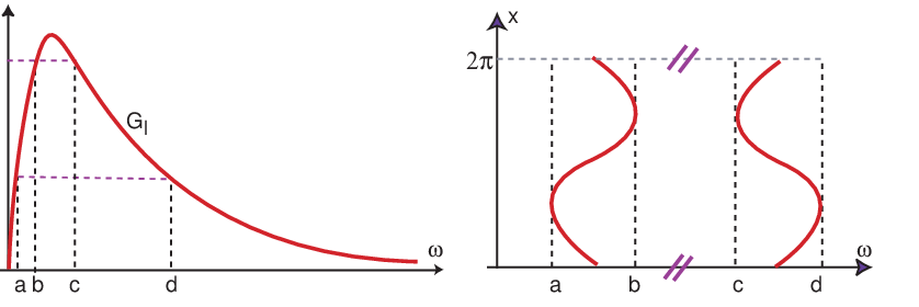
As illustrated in Figures 8 and 9, finding $(1,\ell)$-fixed points of $\mathcal{F}_{\mu}$ amounts to intersect the graph of $\varphi(x)$ with a horizontal line. The line moves first up and then down, as $\omega$ increases. Since the range of $\varphi$ is the interval $\left[A-\lambda,A+\lambda\right]$, and the range of $G_{\ell}(\omega)$ is the interval $\left(0,M\right]$, the geometry of the solution set depends on the relative positions of these intervals. From now on, we use the inequality $M\geq A+\lambda$, $A\in[0,\varepsilon]$ – see (3.1). The analytic treatment of the other cases are similar to the approach of Section 5 of [39].

As $\omega$ increases from $0$, there is a threshold value $\omega_{1}$ for which the horizontal line at height $G_{\ell}(\omega_{1})$ touches the graph of $\varphi$ at $x=3\pi/2$. At this point we have $\sin(x)=-1$. As $\omega$ increases further, each tangency unfolds as two intersection points of the graph with the horizontal line. There is a saddle-node at the points $\left(x^{(1)},G_{\ell}(\omega_{1})\right)=\left(3\pi/2,\,G_{\ell}(\omega_{1})\right)$, as we will see in Proposition 5.2. The surface $G_{\ell}(\omega)=A\pm\lambda$ defines the boundaries of the $(1,\ell)$–resonance wedge. The horizontal line may move further up and a pair of solutions come together at a second saddle-node at $\left(x^{(2)},G_{\ell}(\omega_{2})\right))=\left({\pi}/{2},G_{\ell}(\omega_{2})\right)$ and reappear at a saddle-node at $\left(x^{(3)},G_{\ell}(\omega_{3})\right)=\left({\pi}/{2},G_{\ell}(\omega_{3})\right)$ coming together finally at $\left(x^{(4)},G_{\ell}(\omega_{4})\right)=\left({3\pi}/{2},G_{\ell}(\omega_{4})\right).$ The evolution of the geometry of solutions of (5.4), as $\omega$ varies, is illustrated on the right side of Figure 9. We show below that, at these points, the map $D\mathcal{F}_{\mu}$ has an eigenvalue equal to 1.

References

- [1] V.S. Afraimovich, L.P. Shilnikov. On invariant two-dimensional tori, their breakdown and stochasticity in: Methods of the Qualitative Theory of Differential Equations, Gor’kov. Gos. University (1983), 3–26. Translated in: Amer. Math. Soc. Transl., (2), vol. 149 (1991) 201–212.
- [2] V.S. Afraimovich, S-B Hsu, H. E. Lin. Chaotic behavior of three competing species of May-Leonard model under small periodic perturbations. Int. J. Bif. Chaos, 11(2) (2001) 435–447.
- [3] V. S. Afraimovich, S. B. Hsu. Lectures on Chaotic Dynamical Systems, American Mathematical Society and International Press, 2002.
- [4] M. Aguiar. Vector fields with heteroclinic networks, Ph.D. thesis, Departamento de Matemática Aplicada, Faculdade de Ciências da Universidade do Porto, 2003.
- [5] M.A.D. Aguiar, S.B.S.D. Castro, I.S. Labouriau. Dynamics near a heteroclinic network. Nonlinearity 18 (2005) 391–414.
- [6] A. Algaba, M. Merino, A. Rodríguez-Luis. Takens-Bogdanov bifurcations of periodic orbits and Arnold’s tongues in a three-dimensional electronic model, International Journal of Bifurcation and Chaos 11(02) (2001): 513–531.
- [7] V. Anishchenko, M. Safonova, L Chua. Confirmation of the Afraimovich-Shilnikov torus-breakdown theorem via a torus circuit. IEEE Transactions on Circuits and Systems I: Fundamental Theory and Applications, 40(11) (1993) 792–800.
- [8] V. Arnold. Small denominators. I. Mapping the circle onto itself, Izvestiya Rossiiskoi Akademii Nauk. Seriya Matematicheskaya 25(1) (1961) 21–86.
- [9] D. Arrowsmith, J. Cartwright, A. Lansbury, C. Place. The Bogdanov map: Bifurcations, mode locking, and chaos in a dissipative system, International Journal of Bifurcation and Chaos 3.04 (1993): 803–842.
- [10] D. Aronson, M. Chory, G. Hall, R. McGehee. Bifurcations from an invariant circle for two-parameter families of maps of the plane: a computer-assisted study, Communications in Mathematical Physics, 83(3) (1982) 303–354.
- [11] P. Ashwin, P. Chossat. Attractors for robust heteroclinic cycles with continua of connections, Journal of Nonlinear Science, 8(2) (1998) 103–129.
- [12] I. Baldomá, S. Ibáñez, T. Seara. Hopf-Zero singularities truly unfold chaos, Commun. Nonlinear Sci. Numer. Simul. 84 (2020), 105162.
- [13] T. Bakri, F. Verhulst. Bifurcations of quasi-periodic dynamics: torus breakdown. Zeitschrift für angewandte Mathematik und Physik 65.6 (2014) 1053–1076.
- [14] T. Bakri, Y. Kuznetsov, F. Verhulst. Torus bifurcations in a mechanical system, Journal of Dynamics and Differential Equations, 27 (3-4), (2015) 371–403.
- [15] P. L. Boyland. Bifurcations of circle maps: Arnold tongues, bistability and rotation intervals. Commun. Math. Phys., 106 (1986) 353–381.
- [16] H. Broer, R. Roussarie, C. Simó. Invariant circles in the Bogdanov-Takens bifurcation for diffeomorphisms, Ergod. Th. & Dynam. Sys. 16 (1996) 1147–1172.
- [17] H. Broer, C. Simó, J. C. Tatjer. Towards global models near homoclinic tangencies of dissipative diffeomorphisms Nonlinearity 11 (1998) 667–770.
- [18] V.V. Bykov. On systems with separatrix contour containing two saddle-foci. J. Math. Sci. 95 (1999) 2513–2522.
- [19] V.V. Bykov. Orbit Structure in a neighborhood of a separatrix cycle containing two saddle-foci. Amer. Math. Soc. Transl. 200 (2000) 87–97.
- [20] M. J. Capiński, E. Fleurantin, J. M. James. Computer assisted proofs of two-dimensional attracting invariant tori for ODEs, Discrete & Continuous Dynamical Systems-A, 2020 (to appear)
- [21] M. L. Castro, A. A. P. Rodrigues. Torus-breakdown near a Bykov attractor: a case study, International Journal of Bifurcation and Chaos (2021), to appear.
- [22] A. Denjoy. Sur les courbes définies par les équations différentielles a la surface du tore, J. Math. Pures Appl. 11 (1932) 333–375.
- [23] P. Gaspard. Local birth of homoclinic chaos, Physica D: Nonlinear Phenomena, 62(1-4) (1993) 94–122.
- [24] S.V. Gonchenko, L.P. Shilnikov, D.V. Turaev. Quasiattractors and homoclinic tangencies. Computers Math. Applic. 34(2–4) (1997) 195–227.
- [25] B. Greenspan, P. Holmes. Repeated resonance and homoclinic bifurcation in a periodically forced family of oscillators, SIAM journal on mathematical analysis 15.1 (1984) 69–97.
- [26] J. Guckenheimer, P. Holmes. Nonlinear Oscillations, Dynamical Systems, and Bifurcations of Vector Fields. Applied Mathematical Sciences 42, Springer-Verlag, 1983.
- [27] M. Herman. Mesure de Lebesgue et Nombre de Rotation, Lecture Notes in Math., vol. 597, Springer, (1977) 271–293.
- [28] M. Herman. Sur la conjugaison différentiable des difféomorphismes du cercle à des rotations, Publications Mathématiques de l’IHÉS 49 (1979) 5–233.
- [29] M. W. Hirsch C. Pugh, M. Shub. Invariant manifolds. Bull. Amer. Math. Soc. 76, no. 5 (1970) 1015–1019.
- [30] A.J. Homburg, B. Sandstede. Homoclinic and Heteroclinic Bifurcations in Vector Fields. Handbook of Dynamical Systems 3, North Holland, Amsterdam (2010) 379–524.
- [31] S. Kim, R. MacKay, J. Guckenheimer. Resonance regions for families of torus maps, Nonlinearity, 2(3) (1989) 391–404.
- [32] V. Kirk. Merging of resonance tongues, Physica D: Nonlinear Phenomena 66. 3-4 (1993) 267–281.
- [33] V. Kirk, A. Rucklidge. The effect of symmetry breaking on the dynamics near a structurally stable heteroclinic cycle between equilibria and a periodic orbit, Dynamical Systems 23.1 (2008) 43–74.
- [34] S. Kiriki, T. Soma. Takens’ last problem and existence of non-trivial wandering domains, Advances in Mathematics, 306 (2017) 524–588.
- [35] J. Knobloch, J.S.W. Lamb, K.N. Webster. Using Lin’s method to solve Bykov’s problems. J. Diff. Eqs. 257(8) (2014) 2984–3047.
- [36] I.S. Labouriau, A.A.P. Rodrigues. Global generic dynamics close to symmetry. J. Diff. Eqs. 253(8) (2012) 2527–2557.
- [37] I.S. Labouriau, A.A.P. Rodrigues. Dense heteroclinic tangencies near a Bykov cycle, J. Diff. Eqs. 259(12) (2015) 5875–5902.
- [38] I.S. Labouriau, A.A.P. Rodrigues. Global bifurcations close to symmetry. J. Math. Anal. Appl. 444(1) (2016) 648–671.
- [39] I.S. Labouriau, A.A.P. Rodrigues. Bifurcations from an attracting heteroclinic cycle under periodic forcing, J. Diff. Eqs. 269(5) (2020) 4137–4174.
- [40] W. F. Langford. Numerical studies of torus bifurcations. In: Numerical Methods for Bifurcation Problems. Birkhäuser, Basel, 1984. 285–295.
- [41] L. Mora, M. Viana. Abundance of strange attractors, Acta Math. 171(1) (1993) 1–71.
- [42] S.E. Newhouse. The abundance of wild hyperbolic sets and non-smooth stable sets for diffeomorphisms. Publ. Math. Inst. Hautes Études Sci. 50 (1979) 101–151.
- [43] S. Ostlund, D. Rand, J. Sethna, E. Siggia. Universal properties of the transition from quasi-periodicity to chaos in dissipative systems. Physica D: Nonlinear Phenomena, 8(3), (1983) 303–342.
- [44] I.M. Ovsyannikov, L.P. Shilnikov. On systems with a saddle-focus homoclinic curve. Math. USSR Sb. 58 (1987) 557–574.
- [45] A. Passeggi, R. Potrie, M. Sambarino. Rotation intervals and entropy on attracting annular continua, Geometry & Topology 22(4) (2018) 2145–2186.
- [46] B. Peckham. The necessity of the Hopf bifurcation for periodically forced oscillators, Nonlinearity 3.2 (1990) 261–280.
- [47] B. Peckham, C. Frouzakis, I. Kevrekidis. Bananas and banana splits: a parametric degeneracy in the Hopf bifurcation for maps. SIAM Journal on Mathematical Analysis, 26(1) (1995) 190–217.
- [48] B. Peckham, I. Kevrekidis. Lighting Arnold flames: resonance in doubly forced periodic oscillators, Nonlinearity 15 (2002) 405–428.
- [49] A.A.P. Rodrigues. Persistent switching near a heteroclinic model for the geodynamo problem. Chaos, Solitons & Fractals 47 (2013) 73–86.
- [50] A.A.P. Rodrigues. Repelling dynamics near a Bykov cycle. J. Dyn. Diff. Eqs. 25(3) (2013) 605–625.
- [51] A. A. P. Rodrigues. Strange attractors and wandering domains near a homoclinic cycle to a bifocus, Journal of Differential Equations, 269(4) (2020), 3221–3258.
- [52] A.A.P. Rodrigues. Unfolding a Bykov attractor: from an attracting torus to strange attractors, J. Dyn. Diff. Eqs. 2020 https://doi.org/10.1007/s10884-020-09858-z.
- [53] D. Ruelle, F. Takens. On the nature of turbulence, Les rencontres physiciens-mathématiciens de Strasbourg-RCP25 12 (1971) 1–44.
- [54] A. Shilnikov, G. Nicolis, C. Nicolis. Bifurcation and predictability analysis of a low-order atmospheric circulation model, Internat. J. Bifur. Chaos Appl. Sci. Engrg 5(06), (1995) 1701-1711.
- [55] A. Shilnikov, L. P. Shilnikov, D. Turaev. On some mathematical topics in classical synchronization. A tutorial., Internat. J. Bifur. Chaos Appl. Sci. Engrg. 14 (2004) 2143–2160.
- [56] Q Wang, A. Oksasoglu. Dynamics of homoclinic tangles in periodically perturbed second-order equations, J. Diff. Eqs. 250(2) (2011) 710–751.
- [57] Q. Wang, L.S. Young. From Invariant Curves to Strange Attractors, Commun. Math. Phys. (2002) 225–275.
- [58] K. Yagasaki. Melnikov’s method and codimension-two bifurcations in forced oscillations, J. Differential Equations, 185 (2002) 1–24.
Appendix A Glossary
We record a miscellaneous collection of terms and terminology that are used throughout the text. For small, consider the 3-parameter family of –smooth autonomous differential equations