Construction of low-energy symmetric Hamiltonians and Hubbard parameters for twisted multilayer systems using ab-initio input
Abstract
A computationally efficient workflow for obtaining the low-energy symmetric tight-binding Hamiltonians for twisted multilayer systems is presented in this work. We apply this scheme to twisted bilayer graphene at the first magic angle. As initial step, the full-energy tight-binding Hamiltonian is generated by the Slater-Koster model with parameters fitted to ab-initio data at larger angles. Then, the low-energy symmetric four-band and twelve-band Hamiltonians are constructed using the maximum-localization procedure subjected to crystal and time-reversal-symmetry constraints. Finally, we compute extended Hubbard parameters for both models within the constrained random phase approximation (cRPA) for screening, which again respect the symmetries. The relevant data and results of this work are freely available via an online repository. Our workflow, exemplified in this work on twisted bilayer graphene, is straightforwardly transferable to other twisted multi-layer materials.
I Introduction
The discovery of correlated insulating states and superconductivity in twisted bilayer graphene (TBG) Cao et al. 2018a; Cao et al. 2018b; Kim et al. 2017 has rapidly opened the field of twistronics with stacked van der Waals materials. In TBG at the so-called first magic twist angle , nearly flat bands around the Fermi level emerge, which is the key ingredient for strongly-correlated states to emerge in an otherwise weakly-correlated material Cao et al. 2018a; Xie et al. 2019; Yankowitz et al. 2019; Kerelsky et al. 2019; Lu et al. 2019; Lisi et al. 2021. The observation of a correlated insulator in close proximity to superconductivity further leads one to believe that the superconductivity is of an unconventional nature.
For a theoretical investigation of the phenomena observed in TBG, two ingredients are essential: (1) a faithful description of the low-energy band structure and (2) the form and approximate strength of the relevant interactions. However, performing ab-initio calculations—a standard procedure for finding effective models, such as tight-binding (TB) models—is challenging as the unit cell at the magic angle of contains about twelve thousand atoms, which is prohibitively large for such first-principles calculations. While ab-initio calculations to obtain the full bandstructure were carried out in Ref. Lucignano et al. 2019, the required computational cost places strong constraints on the pseudopotentials and the computational flow. Therefore, simplified schemes for the derivation of effective models in twisted heterostructures are highly desirable.
The simplest approach to describe the (non-interacting) electronic states of TBG is given by the so-called continuum theory or approximation Lopes dos Santos et al. 2007; Koshino et al. 2018; Bistritzer and MacDonald 2011; Bernevig et al. 2020a. Starting from the linearly dispersing Hamiltonian of individual graphene sheets and adding interlayer couplings, the resulting models give a reasonable approximation to the electronic energy dispersion of TBG at arbitrary angles. In addition, the models respect the symmetry group which protects the Dirac points Zou et al. 2018. Even though the method is straight forward to implement, the resulting models ignore quantitative microscopic details, which may alter the qualitative nature of electronic states, including their symmetry or topology.
Another approach is to directly start from a microscopic TB model as an approximate but compact representation of the full, experimentally realistic Hamiltonian in a basis of localized Wannier orbitals. For graphene, the orbital character of states near the Fermi level is dominated by orbitals, which remains true in TBG. For fixed orbital shape and orientation, the standard method for obtaining the hopping parameters of the TB Hamiltonian is to assume the Slater-Koster (SK) analytic form with standard values for the SK parameters Koshino et al. 2018; Trambly de Laissardière et al. 2012; De Trambly Laissardière et al. 2010; Goodwin et al. 2019a; Goodwin et al. 2019b; Haddadi et al. 2020. While this approach allows one to describe systems with unit-cell sizes relevant for small twist angles, the fixed choice of SK parameters restricts the overall accuracy of the scheme.
In this work, we consider a compromise between accuracy and computational cost. Instead of computing the ab-initio TB model at the magic angle, we first optimize the SK parameters according to the ab-initio TB parameters calculated at larger twist angles. The resulting SK parameters are then used for a TB description for TBG at smaller twist angles. In other words, the SK analytic form is used to extrapolate ab-initio information from larger angles to smaller angles. This procedure allows for a significant reduction in computational cost due to the smaller unit cells. We verify the consistency of our approach by comparing the SK parameters obtained using different twist angles. Note that this scheme can also be applied to other twisted multi-layer materials.
The full TB description is not directly amenable towards a many-body analysis due to the huge number of degrees of freedom stemming from the large unit cell close to the magic angle. Therefore, the next step is to construct a minimal, non-interacting low-energy Hamiltonian, which describes the few relevant bands near the Fermi level. We build the low-energy TB Hamiltonians from the SK bandstructures, using the projection method adopted in the Wannier90 software Pizzi et al. 2020. Since the flat bands of TBG are isolated from others, and a good trial orbital set to initiate the procedure is known Kang and Vafek 2019, a four-band TB model can, thus, be easily obtained.
Even at the magic angle the gap between the flat bands to other bands is small (experimentally, meV Zou et al. 2018) compared to, for example, the phonon bandwidth ( meV Choi and Choi 2018). Thus, to study electron-phonon interactions it is desirable to include additional bands close to the Fermi level. Without a gap separating these additional bands from the rest of the spectrum, the Wannierization requires an appropriate ‘disentanglement’ step to separate the Hilbert space of the desired energy range from that of the rest of the band structure. This construction of a low-energy Hamiltonian is non-trivial, though recently, a solution was proposed requiring a multi-step projection procedure to obtain a good Wannier basis Carr et al. 2019. In this work, we report an alternative and simpler procedure to obtain a twelve-band low-energy Hamiltonian, using the standard routines available in the Wannier90 package Pizzi et al. 2020, and a simple modification of the code to include time-reversal (TR) symmetry. We further provide the Wyckoff positions and symmetry representations of Wannier orbitals required for stable convergence of the crystal-symmetry related Wannier90 subroutines and the Wannierization procedure itself.
Note that two possible configurations of commensurate unit cells for TBG exist: The unit cells possess either or symmetry, obtained by rotating -stacked graphene sheets around carbon centers or hexagon centers, respectively. In the latter case, a Wannier obstruction was reported, which would hinder the construction of a four-band tight-binding Hamiltonian with well-defined symmetry transformation of the basis Wannier functions due to the fragile topological nature of the flat bands Zou et al. 2018; Po et al. 2018a; Po et al. 2018b; Po et al. 2019. In the -symmetric case, which we focus on in this article, no such obstruction exists even in the single-valley theories, and a well-localized, symmetric four-band TB model can be obtained 11 1 Note that a successful Wannierization of narrow bands of TBG within the continuum model was reported recently Cao et al. 2021, where both TBG valleys were considered. Therefore, the fragile topological nature of the low-energy Wannier bands may be an artifact of the single-valley approximation, and, therefore, the -symmetric models can be obtained in the future by the proposed workflow as well..
To provide not only the single-particle Hamiltonian but also electron-electron interactions, we further require the form of the extended Hubbard parameters Koshino et al. 2018; Goodwin et al. 2019a; Goodwin et al. 2019b; Bernevig et al. 2020b. To take into account electronic screening, we make the constrained random phase approximation (cRPA), in which the considered low-energy manifold is excluded from the screening process. We compute these parameters for both a four-band and twelve-band low-energy model, and discuss the symmetry constraints they obey.
The remainder of this article is organized as follows: In Sec. II, the full workflow to construct a low-energy effective tight-binding model starting from the extraction of the SK parameters to the projection to four and twelve bands is described. Section III describes the cRPA calculation and Sec. IV shows the results, while Sec. V concludes our work.
II Construction of Tight-binding models
In this section, we describe our workflow of constructing tight-binding models for TBG. We start from ab-initio data at a large, commensurate twist angle () to construct a TB model via a procedure known as Wannierization. The resulting hopping amplitudes are fitted using the SK analytic form. These fitted SK parameters can then be used to construct the TB model at the magic angle, thus allowing us to bypass the expensive step of Wannierizing ab-initio data at the magic angle. Finally, having obtained the TB model at the magic angle, a second Wannierization step is used to obtain the low-energy (four-band and twelve-band) TB Hamiltonians. The full scheme is depicted in Fig. 1. In the rest of the section, we give a detailed explanation of each step in the procedure.

II.1 Wannierization procedure
We first discuss the Wannierization, the process of creating a TB Hamiltonian, which describes a desired manifold of given Bloch states. If the desired set of bands is isolated from other bands at all points in the Brillouin zone, the procedure proceeds simply by finding the set of maximally-localized Wannier orbitals related to the original Bloch function via a Fourier and unitary transformation,
| (1) | |||||
where the sum runs over momenta in the Brillouin zone, are unitary matrices, which mix the Bloch states at each , and are the unit cell position vectors with the so-called home unit cell located at the origin (). The matrices are chosen such that the spread
| (2) |
is minimized. Here is the position operator. The spread can be decomposed into two positive-definite components
| (3) |
where is gauge-independent while is gauge-dependent. When the target bands are isolated, only the gauge-dependent part needs to be minimized since the gauge-independent part is invariant under unitary transformation. Technically, this minimization is achieved using a steepest descent algorithm, for which one needs to compute the gradient
| (4) |
where the antihermitian generates the infinitesimal gauge transformation as Marzari and Vanderbilt 1997; Pizzi et al. 2020. At each iteration, the unitary transformation is updated according to
| (5) |
with step variable .
In the case of entangled bands Souza et al. 2001, i.e., when the target set of bands is not energetically separated from other bands in the entire Brillouin zone, the above procedure has to be augmented with a disentanglement step. This step ensures that at each point the smoothest set of Bloch wavefunctions is selected from a larger set of size Pizzi et al. 2020,
| (6) |
Here, are semi-unitary matrices (), chosen such that the gauge-invariant spread computed on is minimized. Technically, this results in an iterative procedure, where at each iteration the mismatch of Hilbert subspaces, and , where runs over all momentum points nearest to , is minimized for all .
In this work, we use an additional restriction in the disentanglement procedure Souza et al. 2001: in Sec. II.5 we choose an energy range within which the original Bloch manifold must be exactly reproduced. This energy range is called the inner, or frozen window of the disentanglement procedure. In this case, the manifold of Bloch states within the frozen window is fixed and always contained in .
Due to the non-convex nature of the optimizations, the initialization of the various iterative procedures plays a critical role. This initialization is achieved by choosing a set of trial orbitals. Given the trial orbitals, the initial value of the matrices and can then be defined in the following way. First, one expands the projection above back onto the Hilbert space of interest
| (7) |
where
| (8) |
Next, by orthonormalizing, we obtain a set of Bloch states, in the sense of or from Eqs. (1) and (6), respectively:
| (9) | |||||
| (10) |
where . The matrices then serve for initialization of and in the maximum-localization and disentanglement algorithm, respectively. When the trial orbitals are chosen appropriately, this initial guess for is often used for TB model construction, i.e., without performing maximum localization. In Sec. II.5, we make use of such a one-step procedure after obtaining a converged disentangled manifold.
After obtaining the and matrices, the TB Hamiltonian can be constructed by rotating the initial eigenvalues as or in the entangled-bands case. Here, is the matrix with the energy eigenvalues on the diagonal, and zero entries otherwise. Then, the subsequent (inverse) Fourier transform to real space gives the desired set of hopping parameters , such that the translationally invariant TB Hamiltonian in second quantized form reads
| (11) |
where are second quantized operators, which create (annihilate) a Wannier orbital (see Eq. (1)) located at position with being the position of orbital within the unit cell.
II.2 Crystal symmetry constraint
The Wannierization procedure defined above preserves neither crystal nor TR symmetries. For the procedure to respect these symmetries, we place a constraint on the matrices and during the maximal-localization and disentanglement procedures, respectively Sakuma 2013; Pizzi et al. 2020.
To simplify the notations, we restrict ourselves to working with the point group only, which is possible in TBG by choosing the unit cell appropriately. In the space of Bloch states the symmetry representation matrix for a point group element is defined through
| (12) |
where the action of in euclidean space is expressed as . On the other hand, the corresponding Wannierized states have to obey a similar transformation rule
| (13) |
with desired symmetry representation matrices , which are block diagonal, and each block corresponds to a site-symmetry-induced irreducible representation determined from the chosen orbital configuration of the TB model. The exact definitions of and can be found in Ref. Sakuma 2013. It can be shown that for a point group operation in the little group —the subgroup of which leaves a given unchanged—the following relationship holds Sakuma 2013
| (14) |
for the matrices from Eq. (1) (exactly the same equation must hold for the matrices from Eq. (6) in the entangled-bands case). Starting from the initial guess, this equation is solved iteratively to ensure that the symmetry condition holds. Note, that Eq. (14) can only be satisfied if the irreducible representations of original and the targeted Wannierized Bloch manifolds Sakuma 2013 are compatible in the targeted energy window.
In the subsequent steepest descent optimization of the maximum localization procedure, the gradient in Eq. (4) is replaced by
| (15) |
where is the order of the little group , in order to preserve the equality (14) at every iteration. One only needs to solve Eq. (14) on an irreducible wedge of momentum points, while at other momentum points is constructed by applying the symmetry transformations. A similar approach is used at the disentanglement step Sakuma 2013; Pizzi et al. 2020.
II.3 Time-reversal symmetry constraint
In spinless systems with TR symmetry, a real basis of maximally-localized Wannier orbitals is guaranteed to exist. While Wannier90 code usually manages to find such real Wannier orbitals, this is generally not guaranteed. Particularly in TBG, this symmetry tends to be broken when constructing low-energy TB models. The TR-symmetric four-band low-energy model can be obtained by considering a set of complex TR-related pairs as trial orbitals Kang and Vafek 2018, and skipping the maximum-localization procedure. Either when using maximum localization or an odd number of such complex orbitals at some sites (as in our twelve-band model below), the TR symmetry can not be fixed explicitly by available software, and therefore can be broken in the resulting TB Hamiltonian. In this work, we implement a scheme, which allows for explicit TR symmetry constraint in both disentanglement and maximum-localization steps, involving only a minor modification of Wannier90 code, and requiring no additional input.
First, we fix the arbitrary phase of eigenvectors of the original band structure to satisfy the TR symmetry constraint. Neglecting the spin degrees of freedom, this is achieved by only taking eigenvectors in the irreducible wedge of points with respect to the TR operator and constructing the eigenvectors at point via
| (16) |
where the TR operator , the complex conjugation. If the unitary matrices and satisfy the condition
| (17) |
where corresponds to either or , the resulting Wannier orbitals will be real. This condition can be satisfied by the substitution
| (18) |
However, the operation in Eq. (18) breaks unitarity (for ) or semi-unitarity (for ) of the matrices, which has to be restored with an “orthonormalization” subroutine available within the Wannier90 software.
Interestingly, it is only necessary to make the replacement Eq. (18) in the final iteration of the maximum localization procedure. In this way, the replacement does not significantly affect the spread of the resulting Wannier orbitals and also preserves the crystal symmetries, discussed in Sec. II.2, accurately. On the other hand, for the disentanglement procedure, it is necessary to apply the substitution at every iteration. Further details regarding the symmetrization are provided in the appendix.
II.4 Slater-Koster parametrization
The hopping amplitudes of a TB Hamiltonian are often well described by the SK analytic form Slater and Koster 1954. The analytic structure depends only on the geometric configuration, character of basis orbitals, and a set of fitting parameters. This approach was successfully applied to TBG by considering carbon’s orbitals only with the following analytic form for the hopping amplitudes in the corresponding TB model Koshino et al. 2018; Trambly de Laissardière et al. 2012; De Trambly Laissardière et al. 2010; Goodwin et al. 2019a; Goodwin et al. 2019b; Haddadi et al. 2020:
| (19) |
where , is the component of , is the in-plane carbon-carbon bond length, and is the interlayer distance. The SK parameters , , and , are typically fixed to eV, eV, and , respectively.
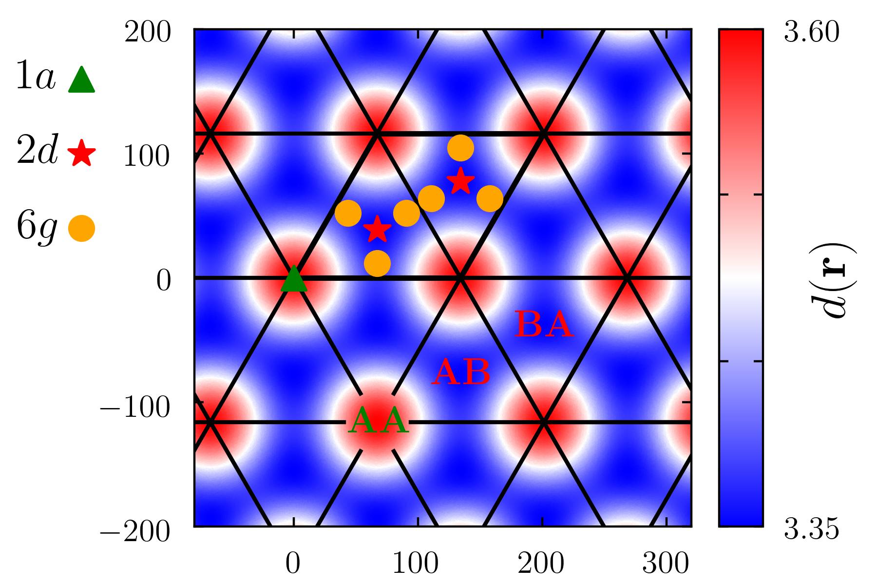
Due to its analytic form, the SK approach can be directly applied to handle the atomic relaxations specific to TBG. In this work, we consider only out-of-plane corrugations Uchida et al. 2014, in which the distance between layers varies from in AA stacked regions to in AB stacked regions. Here, AA (AB) stacking refers to regions where the same (opposite) sublattice atoms of the two graphene layers align. We use a smooth interpolation between these values, such that at the atomic site , we have an interlayer separation
| (20) | |||||
where , with Å and Å Uchida et al. 2014; Koshino et al. 2018, see Fig. 4. Although the average magnitude of the in-plane and out-of-plane relaxations are similar in magic-angle TBG, our model of out-of-plane-only lattice corrugations yields a bandstructure very similar to the fully DFT-relaxed crystal structure of Ref. Cantele et al. 2020. As the corrugations generated by Eq. (20) preserve the symmetries, we use this model in all our calculations. A comparison of different crystal structures and their corresponding electronic bands is shown in the Appendix D.
II.5 Extraction of hopping parameters from ab-initio calculation for TBG
Usually, the SK parameters defining the hopping amplitudes in Eq. (19) are fixed to the values given in Sec. II.4. However, this places a clear restriction on the accuracy of the resulting model. Therefore, we propose to Wannierize ab-initio data at larger twist angles and use the resulting hopping amplitudes to extract the SK parameters. We assume that the parameters extracted at large twist angles are still a good approximation for smaller angles. This way, we do not have to perform the expensive Wannierization using ab-initio data at the magic angle.
We start by rewriting the TB Hamiltonian to distinguish between the in-plane () and out-of-plane () hopping terms,
| (21) |
where and denotes the Heaviside step function. The argument of the Heaviside step function allows to distinguish in-plane hopping with finite -component from purely out-of plane components in the case of corrugated layers.
The TB parameters can then be obtained from the ab-initio calculations by Wannierization of the DFT Bloch manifold, as discussed in Sec. II.1. Following Eq. (19), the hopping coefficients depend on the displacement connecting the corresponding sites.
Since the vertical component of is small for in-plane hoppings, especially at small distances due to the long-wavelength nature of atomic corrugations, one may assume that the corresponding in-plane hopping amplitudes are only of -type and identical to those in single-layer graphene (SLG). Furthermore, the weak van der Waals forces of the interlayer coupling should only have a minor effect on the in-plane Hamiltonian of each individual layer of TBG. Still, we use the standard SK parametrization for the in-plane TB Hamiltonian in TBG, and find that together with our new out-of-plane parameterization (below) it produces the right bandstructures with the crystal structure defined in Eq. (20) and the DFT-relaxed crystal structure from Ref. Cantele et al. 2020 (see Appendix D for more details) 22 2 Direct wannierization leads to a different sign of the second-nearest neighbor interaction in comparison with the first nearest-neighbor one appearing in the SLG ab-initio TB model. This sign structure of the TB parameters is confirmed in other works on the Wannierization of the DFT bandstructures for the SLG Jung and MacDonald 2013; Jung and MacDonald 2014. This is in contrast to fitting the DFT bandstructure (e.g. in Ref. Reich et al. 2002), which produces a TB model with hopping amplitudes all being negative up to the third nearest-neighbor, which probably can be achieved with the maximum localization algorithm as well subjected, however, to another constraint.
For the computation of the out-of-plane hopping amplitudes , we follow a different path: Since the number of non-equivalent matrix elements of this type is very large at small twist angles, our approach is to () perform the Wannierization at larger twist angles (smaller unit cell), () get the list of all possible out-of-plane hopping amplitudes for this case, and () fit this data to the SK analytic expression. We apply this scheme to TBG at the largest and the second-largest commensurate twist angles and , respectively. Finally, the resulting analytic expression for is used to construct the full TB Hamiltonian for TBG at arbitrary commensurate twists.
Since the maximum-localization procedure shifts, in general, the final Wannier-orbital centers from their original positions, we skip this step, i.e., the spread given in Eq. (3) is not minimized, and the corresponding matrices are to be defined as described at the end of Sec. II.1. In addition, the disentanglement was done with the frozen window technique. The choice of the frozen window in both calculations is shown in Fig. 2 with respect to the original DFT bandstructure. The Wannierized bandstructure is also shown in that figure.
II.6 Low-energy models
The SK Hamiltonian described above is still large ( matrix per point), but can be exactly diagonalized as a non-interacting problem. Accounting for interactions, however, increases the computational costs exponentially. For many-body calculations, a smaller basis set is highly desirable. The most natural way to achieve such a smaller basis set is to perform a further Wannierization of the non-interacting TB Hamiltonian for TBG, such that the resulting model only contains bands close to the Fermi level. Unlike for the construction of the ab-initio TB models above, we use a maximum localization procedure subjected to the crystal and time-reversal-symmetry constraints for the construction of the low-energy models. The specific details on the choice of trial-orbital configurations are described in two sections below.

II.6.1 Four-band Hamiltonian
Since the four flat bands of magic angle TBG are isolated from all other bands, the Wannierization to a four-band model is straight forward. It is known Kang and Vafek 2018 that a good trial orbital set, in Eq. (8), is obtained by taking linear combinations of the Bloch wavefunctions at the point and truncating with Gaussians centered at the AB or BA site. In addition, we impose the crystal symmetry constraint on the Wannierization procedure as discussed in Sec. II.2. In contrast to Ref. Kang and Vafek 2018, where complex orbitals are obtained, our target symmetry representation matrices are obtained by assuming that the Wannier functions transform as real atomic orbitals located at AB and BA sites of the TBG unit cell. Real orbitals are obtained by adding the constraint of time-reversal symmetry as described in Sec. II.3. Following an earlier study in Ref. Koshino et al. 2018, we justify this choice by the correct irreducible representations of the Bloch bands at the and points in the Brillouin zone under the symmetry group (which we exclusively deal with in this article).
II.6.2 Twelve-band Hamiltonian
Given the small (computed as meV) band gaps between the flat bands and the rest of the band structure, the inclusion of at least the next eight bands may be relevant for many-body physics. The problem, however, is that some of these additional bands are entangled, i.e., degenerate or crossing, with higher or lower bands. Therefore, an additional disentanglement step is needed to construct a smooth manifold of Bloch states in momentum space for subsequent maximum localization.
Reference Carr et al. 2019 proposed a multistep projection scheme for constructing the trial set of orbitals. The main disadvantage of this scheme is that one has to work with a valley-projected bandstructure, which is generally not the result of ab-initio calculations. Secondly, the number of resulting Wannier orbitals is strongly constrained. Two orbitals are needed for flat bands and three orbitals are needed for each lower and upper lowest-energy (non-flat) subset of bands. As a result, one can work with either or bands per valley.
The approach we shall take, on the other hand, is not subject to such restrictions. We simply choose a trial orbital set , which has a good overlap with the wavefunctions of the SK bandstructure close to the Fermi level, and delegate the search for the optimal Wannier orbitals to the Wannierization procedures described in Sec. II.1 with crystal and time-reversal symmetry constraints, using the Wannier90 code. In particular, the trial orbitals in the twelve-band case are computed from the wavefunctions at in the following way. Consider the twelve bands closest to the Fermi level, labelling them in order of increasing energy. Next, the bands with indices and are paired together. The trial orbitals are then formed by combining the pairs and . In addition, these trial orbitals are truncated by Gaussians centered along the center of rotation of the corresponding irreducible representation. A similar approach was recently taken in the four-band case Kang and Vafek 2018. Details on the symmetry configuration are discussed in Sec. IV.2.
III Interactions
Having obtained the non-interacting low-energy model, the final ingredient for a full many-body Hamiltonian is to consider the Coulomb interaction between electrons. In general, this interaction is screened by the surrounding media, which in our case comprises all electrons that do not enter the low-energy Hamiltonian, and by an environmental dielectric function accounting for the substrate on which TBG is placed. A straightforward way to take into account this screening is by making the constrained random phase approximation (cRPA) which we describe below.
After computing the screening, one can then compute the Hubbard parameters in order to construct the many-body Hamiltonian. These parameters simply correspond to matrix elements of the cRPA-screened Coulomb interaction in the Wannier basis of the low-energy TB model. The workflow for calculating theses quantities is described in the subsequent sections and follows very closely that of Ref. Goodwin et al. 2019a, with the exception that symmetries are taken into account. In addition, we fit the resulting matrix elements with an analytic envelope function to better understand their dependence on distance.
III.1 Screened Coulomb interaction
The cRPA screening is described by the polarizability function
| (22) |
where is a vector in the first Brillouin Zone and is a reciprocal lattice vector. The prime in the second summation indicates that transitions between bands used in the construction of the low-energy Hamiltonian are excluded. The indices and thus run over all conduction and valence bands, respectively, that are not part of the low-energy Hamiltonian. The cRPA dielectric function is then evaluated via
| (23) |
with the bare Coulomb interaction in two dimensions in atomic units and we choose a substrate-specific to simulate screening Goodwin et al. 2019a. The screened Coulomb interaction can then be computed in real space by performing the Fourier transform:
| (24) |
The eigenvalues entering the cRPA polarizability expression in Eq. (22) are computed on a grid of points. In total, 8400 bands were used to ensure convergence. Calculation of the cRPA polarizability for the four-band model is straightforward. One simply needs to exclude four flat bands out of the sum in Eq. (22). The twelve-band model, on the other hand, is constructed with the disentanglement procedure, which forbids the direct use of Eq. (22) in principle. However, due to the fact that the energy range of the twelve-band model spectrum is equal to that of the lowest twelve bands of the original Hamiltonian, we can assume that screening properties of both sets of bands should be similar. Moreover, the resulting disentanglement matrices of Eq. (6) show that the dominant contribution of the final Wannier basis set indeed comes from these twelve bands. Therefore, we use Eq. (22) as given ignoring the twelve bands closest to the Fermi level in the sum, which is straightforward since this set is isolated on the chosen -point grid (the degenerate and Brillouin-zone points are not present on this grid).
III.2 Hubbard parameters
The screened Coulomb interaction computed in the previous section is incorporated into the non-interacting low-energy TB Hamiltonian in the form of two-body interaction terms given by
| (25) |
where is the two-body interaction matrix element. When and , the terms become a density-density interaction and the corresponding parameters are also known as the Hubbard parameters.
Given the Wannier-orbital wave functions as well as the screened interaction obtained in the previous section, the Hubbard parameters can be computed as
| (26) | |||||
The calculation is done by decomposing the Wannier orbitals in the basis of orbitals at each carbon site of TBG
| (27) |
Here are defined from the solution of the free SK-TB Hamiltonian , via the result of the maximum localization procedure
| (28) |
where , the transformation from Eq. (1), always carries a bold momentum superscript, and should not be confused with the Hubbard parameter matrix without such a superscript. In the twelve-band case, the orbitals must be replaced by smoothed from Eq. (6).
Following the approach of Refs. Goodwin et al. 2019b; Goodwin et al. 2019a, we have assumed that carbon orbitals of different sites have zero overlap, such that the final expression for the Hubbard parameters is given by
| (29) | |||||
where .
The summation in Eq. (29) needs to be cut at short distances due to the high computational costs. This leads to a slight error of the sum, and an associated small symmetry breaking of the matrix . Moreover, the calculation of the full matrix as given in Eq. (25) is computationally more challenging. Therefore, we reduce the computation to matrix elements that are not related by symmetry (i.e., an irreducible wedge) and obtain the others via the application of symmetry transformations. Symbolically, this operation can be represented as
| (30) |
where are combined orbital indices (e.g., ), are lattice vectors for general [left hand side of Eq. (30)] and irreducible (right hand side) wedge respectively. is a symmetry operation which connects these matrix elements.
The transformation requires the full interaction matrix parameters defined by
| (31) |
When and , the equation reduces to Eq. (29).
The operation in Eq. (30), and the construction of the irreducible wedge is based on the knowledge of the symmetry transformations of the interaction parameters above, which in turn is based on the knowledge of site-symmetry representations of the Wannier orbitals, and thus, the point group representation matrices . The complete derivation for the symmetry transformations of is presented in Appendix A. Here, we give only the final expression,
| (32) | ||||
where , and tilde is related to the action of the inverse symmetry operation (see Appendix A for details). Note that Eq. (32) can also be used to symmetrize an existing matrix, in a similar fashion as the symmetrization of TB models in Ref. Gresch et al. 2018 (see Appendix A).
IV Results
IV.1 Extraction of TB parameters

All Wannierization calculations were performed with Wannier90 code version 3.1.0 Pizzi et al. 2020. The SIESTA code version 4.0.2 García et al. 2020 was used for DFT calculations, for which a non-relativistic pseudopotential and the local density approximation (LDA) for the exchange-correlation functional was chosen. A and mesh was used in and TBG, respectively. In all cases, the so-called SZ (single-) basis of the SIESTA code was chosen.
Figure 3 shows the in-plane and out-of-plane hopping amplitudes of -TBG, as a function of distance. The values follow the SK analytical form well, albeit not with the standard parameters. In addition, we repeated the procedure using ab-initio data for -TBG. We found that the fitted SK parameters for this case are in good agreement with those computed for -TBG, thus lending credibility for its subsequent use at the magic angle. Fitted Slater-Koster parameters for out-of-plane interactions can be found in Tab. 1. Notably large value of in comparison with its literature value of eV is due to prefactor in Eq. (19), which is small for closest out-of-plane interactions dominating the fit, and a larger value of the fitting parameter is required for a sensible range of the physical hopping parameters [Eq. (21)].
| (eV) | (eV) | |||
|---|---|---|---|---|
| Ref. | -2.7 | 0.48 | 3.14 | 7.43 |
| Fit | -35.7 | 0.31 | 2.56 | 3.29 |
The slight variance of the data away from the SK-fitted line is explained by the fact that the actual electronic orbitals formed within the DFT framework are not strictly aligned along the vertical axes. An alternative scheme was proposed in Ref. Fang and Kaxiras 2016 to include the dependence of the out-of-plane hopping amplitudes between atoms and on the in-plane -bonding directions originating from these atoms. The reported small-angle TBG bandstructure supports a set of flat bands, which, however, is not as well isolated from other bands. This shortcoming has been attributed to neglected lattice relaxation effects. We leave the complete resolution of this question to future research.
IV.2 Low-energy models


In the construction of the four-band low-energy model, we used a -point mesh. The trial orbital set was composed in a similar way as was done in Ref. Kang and Vafek 2018 with a key difference that crystal and time-reversal symmetries were included in our calculations as discussed earlier. These symmetry constraints led to real-valued orbitals which transform as , as opposed to the complex TR-related pairs in Ref. Kang and Vafek 2018. Another advantage of our scheme is that, in principle, one does not need the exactly symmetric trial orbital configuration, because this is fixed during the constrained maximum localization procedure.
In the twelve-band case, the target symmetry configuration of the trial orbital set was chosen according to the one represented by atomic orbital symbols in Fig. 6. It includes six -like orbitals at the , two -like at the , and a pair ( and ) of two-dimensional irreducible representations of at the Wyckoff positions of space group Aroyo et al. 2006. These Wyckoff positions are shown in Fig. 4. This configuration gave a stable convergence of Eq. (14) for several different -point grids. We have chosen a grid for the twelve-band TB model construction.
In both the four- and twelve-band cases, the Wannierization procedure results in exponentially localized Wannier functions as shown in Fig. 5 and Fig. 6, respectively. For the four-band model, the resulting orbital shape is similar to that obtained in Ref. Kang and Vafek 2018. On the other hand, the orbitals obtained for the twelve-band model have very diverse shape. Moreover, it can be seen from Fig. 6 that the center of mass and Wyckoff position do not necessarily match except when the orbitals are centered at AB and BA (honeycomb) sites.
The spread of Wannier basis functions of the four- and twelve-band models can be quantified by computing the average absolute band energy error per band and point with respect to a hopping cutoff (),
| (33) |
This is done by ignoring all hopping amplitudes above a certain threshold, i.e., when the hopping between sites and is ignored. corresponds to including all hopping terms. The result is shown in Fig. 7, and one can clearly see that the twelve-band model has shorter decay length, which can be attributed to the lower spread of orbitals. It is even possible to further reduce the spread of the Wannier orbitals in the twelve-band case by switching off the crystal symmetry constraint and using a frozen window in the disentanglement step. The result of the corresponding calculation is shown in Appendix B.
Finally, we show the bandstructures of the resulting low-energy models in Fig. 8. There is a slight deviation of the twelve-band-model bandstructure around the Dirac points, which does not happen in the four-band case. This is due to the disentanglement step, which mixes bands outside the energy window of interest. This deviation and mixing is, however, very small and can be safely neglected.
IV.3 Hubbard parameters
Hubbard parameters for both models are shown in Fig. 7 (right). Fewer bands are included in the cRPA polarizability summation of Eq. (22) of the twelve-band model in comparison to four-band case, which results in poorer screening. The orbitals are also more compact such that the Hubbard parameters have larger values at short range but decay faster with distance. For the four- and twelve-band models, the interactions become negligible at distances larger than Å and Å, respectively, to be compared to the lattice constant of magic-angle TBG, Å.
It was shown that the Ohno potential Ohno 1964 reasonably describes the dependence of Hubbard parameter values on the inter-orbital distance in TBG Goodwin et al. 2019b; Goodwin et al. 2019a. However, a better fit was achieved in our calculations by considering a soft Coulomb interaction subjected to a Gaussian cut off,
| (34) |
where is the (fixed) on-site Hubbard interaction, while , and are fitting parameters. The fitted values for are meV, , Å, Å and meV, , Å, Å for four- and twelve-band model respectively. The quality of this fit is demonstrated in Fig. 7 (right).
Finally, our exchange parameters, which correspond to taking and in Eq. (31) do not show any long-range behaviour, as seen from the Fig 7. This behaviour is different from the one found in Ref. Cao et al. 2021, and can be due to several reasons. First, we perform the maximum localisation procedure for obtaining the low-energy model. Second, we use full symmetry group instead of one in the reference. Third, our RPA model of screening may behave differently than the gate screening used, most likely, in Ref. Cao et al. 2021. And last, we have used quite comprehensive tight-binding model, while the continuum model was employed in the reference above.
V Conclusions
In this work, we explored a new microscopic approach for obtaining an interacting low-energy tight-binding description of TBG. The two standard microscopic approaches begin either (i) by assuming that the TB hopping amplitudes are described by the SK form with a heuristic choice for the SK parameters or (ii) by performing a full Wannierization of ab-initio DFT data at the magic angle. The former is computationally light but of limited accuracy, while the latter is computationally expensive despite being highly accurate. Our approach takes the middle ground by making a compromise between accuracy and computational cost.
The main idea is to perform Wannierization of ab-initio data not at the magic angle, but at a larger twist angle, thus significantly reducing the computational requirements. The resulting TB model can then be used to extract the SK parameters which allows one to construct a TB model at arbitrary angles. The bandstructure at the first magic angle was further Wannierized to give fully symmetric four- and twelve-band low-energy models. The low-energy Hamiltonians together with their corresponding Hubbard parameters are available at the open repository Davydov et al. 2020.
The full workflow presented in this article attempts to make a fair compromise between accuracy and computational cost. The various techniques and tricks used here are easily applicable and adaptable to any twisted multi-layer system, where the large unit cells present a computational difficulty.
During the course of this work we encountered two questions that might be worth studying in the future. First, the Wannierized ab-initio data does not exactly follow the SK curves for interplane hopping amplitudes. This is most likely due to the assumption of rigid orbitals. Therefore, a potential improvement of the numerical precision of our scheme can be achieved by taking into account such deviations. Secondly, we found that a more compact twelve-band model can be obtained using the so-called frozen window technique when the crystal symmetry constraint is given up. The crystal symmetry constraint within the frozen window calculation is, however, not yet implemented in the Wannier90 code. Implementation of this functionality would allow to study if such scheme would give a better result in comparison to the symmetric twelve-band model presented in the main text. This comparison is left for future research, when such implementation will be available.
Acknowledgement
This work was initiated and motivated by Alexey Soluyanov, who sadly passed away in October 2019.
This research was supported by the NCCR MARVEL, funded by the Swiss National Science Foundation. K.C. is supported by the European Unions Horizon 2020 research and innovation program (ERC-StG-Neupert-757867-PARATOP). We thank Zachary Goodwin and Stepan Tsirkin for useful conversation and sharing the data. Finally, we thank Quansheng Wu and Giovanni Cantele for sharing their atomic structure data.
References
- Cao et al. (2018a) Y. Cao, V. Fatemi, A. Demir, S. Fang, S. L. Tomarken, J. Y. Luo, J. D. Sanchez-Yamagishi, K. Watanabe, T. Taniguchi, E. Kaxiras, R. C. Ashoori, and P. Jarillo-Herrero, Nature 556, 80 (2018a).
- Cao et al. (2018b) Y. Cao, V. Fatemi, S. Fang, K. Watanabe, T. Taniguchi, E. Kaxiras, and P. Jarillo-Herrero, Nature 556, 43 (2018b).
- Kim et al. (2017) K. Kim, A. DaSilva, S. Huang, B. Fallahazad, S. Larentis, T. Taniguchi, K. Watanabe, B. J. LeRoy, A. H. MacDonald, and E. Tutuc, Proceedings of the National Academy of Sciences of the United States of America 114, 3364 (2017).
- Xie et al. (2019) Y. Xie, B. Lian, B. Jäck, X. Liu, C. L. Chiu, K. Watanabe, T. Taniguchi, B. A. Bernevig, and A. Yazdani, Nature 572, 101 (2019), arXiv:1906.09274 .
- Yankowitz et al. (2019) M. Yankowitz, S. Chen, H. Polshyn, Y. Zhang, K. Watanabe, T. Taniguchi, D. Graf, A. F. Young, and C. R. Dean, Science 363, 1059 (2019), arXiv:1808.07865 .
- Kerelsky et al. (2019) A. Kerelsky, L. J. McGilly, D. M. Kennes, L. Xian, M. Yankowitz, S. Chen, K. Watanabe, T. Taniguchi, J. Hone, C. Dean, A. Rubio, and A. N. Pasupathy, Nature 572, 95 (2019).
- Lu et al. (2019) X. Lu, P. Stepanov, W. Yang, M. Xie, M. A. Aamir, I. Das, C. Urgell, K. Watanabe, T. Taniguchi, G. Zhang, A. Bachtold, A. H. MacDonald, and D. K. Efetov, Nature 574, 653 (2019).
- Lisi et al. (2021) S. Lisi, X. Lu, T. Benschop, T. A. de Jong, P. Stepanov, J. R. Duran, F. Margot, I. Cucchi, E. Cappelli, A. Hunter, A. Tamai, V. Kandyba, A. Giampietri, A. Barinov, J. Jobst, V. Stalman, M. Leeuwenhoek, K. Watanabe, T. Taniguchi, L. Rademaker, S. J. van der Molen, M. P. Allan, D. K. Efetov, and F. Baumberger, Nature Physics 17, 189 (2021).
- Lucignano et al. (2019) P. Lucignano, D. Alfè, V. Cataudella, D. Ninno, and G. Cantele, Phys. Rev. B 99, 195419 (2019).
- Lopes dos Santos et al. (2007) J. M. B. Lopes dos Santos, N. M. R. Peres, and A. H. Castro Neto, Physical Review Letters 99, 256802 (2007), arXiv:0704.2128 .
- Koshino et al. (2018) M. Koshino, N. F. Q. Yuan, T. Koretsune, M. Ochi, K. Kuroki, and L. Fu, Phys. Rev. X 8, 031087 (2018).
- Bistritzer and MacDonald (2011) R. Bistritzer and A. H. MacDonald, Proceedings of the National Academy of Sciences of the United States of America 108, 12233 (2011), arXiv:1009.4203 .
- Bernevig et al. (2020a) B. A. Bernevig, Z. Song, N. Regnault, and B. Lian, Tbg i: Matrix elements, approximations, perturbation theory and a 2-band model for twisted bilayer graphene (2020a), arXiv:2009.11301 [cond-mat.str-el] .
- Zou et al. (2018) L. Zou, H. C. Po, A. Vishwanath, and T. Senthil, Physical Review B 98, 085435 (2018), arXiv:1806.07873 .
- Trambly de Laissardière et al. (2012) G. Trambly de Laissardière, D. Mayou, and L. Magaud, Physical Review B 86, 125413 (2012), arXiv:1203.3144 .
- De Trambly Laissardière et al. (2010) G. De Trambly Laissardière, D. Mayou, and L. Magaud, Nano Letters 10, 804 (2010).
- Goodwin et al. (2019a) Z. A. H. Goodwin, F. Corsetti, A. A. Mostofi, and J. Lischner, Physical Review B 100, 235424 (2019a), arXiv:1909.00591 .
- Goodwin et al. (2019b) Z. A. H. Goodwin, F. Corsetti, A. A. Mostofi, and J. Lischner, Physical Review B 100, 121106(R) (2019b).
- Haddadi et al. (2020) F. Haddadi, Q. S. Wu, A. J. Kruchkov, and O. V. Yazyev, Nano Letters 20, 2410 (2020), arXiv:1906.00623 .
- Pizzi et al. (2020) G. Pizzi, V. Vitale, R. Arita, S. Blügel, F. Freimuth, G. Géranton, M. Gibertini, D. Gresch, C. Johnson, T. Koretsune, J. Ibañez-Azpiroz, H. Lee, J.-M. Lihm, D. Marchand, A. Marrazzo, Y. Mokrousov, J. I. Mustafa, Y. Nohara, Y. Nomura, L. Paulatto, S. Poncé, T. Ponweiser, J. Qiao, F. Thöle, S. S. Tsirkin, M. Wierzbowska, N. Marzari, D. Vanderbilt, I. Souza, A. A. Mostofi, and J. R. Yates, Journal of Physics: Condensed Matter 32, 165902 (2020), arXiv:1907.09788 .
- Kang and Vafek (2019) J. Kang and O. Vafek, Physical Review Letters 122, 246401 (2019), arXiv:arXiv:1810.08642v1 .
- Choi and Choi (2018) Y. W. Choi and H. J. Choi, Physical Review B 98, 241412(R) (2018), arXiv:1809.08407 .
- Carr et al. (2019) S. Carr, S. Fang, H. C. Po, A. Vishwanath, and E. Kaxiras, Phys. Rev. Research 1, 033072 (2019).
- Po et al. (2018a) H. C. Po, L. Zou, A. Vishwanath, and T. Senthil, Physical Review X 8, 31089 (2018a), arXiv:1803.09742 .
- Po et al. (2018b) H. C. Po, H. Watanabe, and A. Vishwanath, Physical Review Letters 121, 126402 (2018b), arXiv:1709.06551 .
- Po et al. (2019) H. C. Po, L. Zou, T. Senthil, and A. Vishwanath, Physical Review B 99, 195455 (2019), arXiv:1808.02482 .
- (27) Note that a successful Wannierization of narrow bands of TBG within the continuum model was reported recently Cao et al. 2021, where both TBG valleys were considered. Therefore, the fragile topological nature of the low-energy Wannier bands may be an artifact of the single-valley approximation, and, therefore, the -symmetric models can be obtained in the future by the proposed workflow as well.
- Bernevig et al. (2020b) B. A. Bernevig, Z.-D. Song, N. Regnault, and B. Lian, Tbg iii: Interacting hamiltonian and exact symmetries of twisted bilayer graphene (2020b), arXiv:2009.12376 [cond-mat.str-el] .
- Marzari and Vanderbilt (1997) N. Marzari and D. Vanderbilt, Physical Review B - Condensed Matter and Materials Physics 56, 12847 (1997), arXiv:9707145 [cond-mat] .
- Souza et al. (2001) I. Souza, N. Marzari, and D. Vanderbilt, Phys. Rev. B 65, 035109 (2001).
- Sakuma (2013) R. Sakuma, Phys. Rev. B 87, 235109 (2013).
- Kang and Vafek (2018) J. Kang and O. Vafek, Phys. Rev. X 8, 031088 (2018).
- Slater and Koster (1954) J. C. Slater and G. F. Koster, Physical Review 94, 1498 (1954).
- Uchida et al. (2014) K. Uchida, S. Furuya, J. I. Iwata, and A. Oshiyama, Physical Review B - Condensed Matter and Materials Physics 90, 155451 (2014).
- Cantele et al. (2020) G. Cantele, D. Alfè, F. Conte, V. Cataudella, D. Ninno, and P. Lucignano, Physical Review Research 2, 043127 (2020), arXiv:2004.14323 .
- (36) Direct wannierization leads to a different sign of the second-nearest neighbor interaction in comparison with the first nearest-neighbor one appearing in the SLG ab-initio TB model. This sign structure of the TB parameters is confirmed in other works on the Wannierization of the DFT bandstructures for the SLG Jung and MacDonald 2013; Jung and MacDonald 2014. This is in contrast to fitting the DFT bandstructure (e.g. in Ref. Reich et al. 2002), which produces a TB model with hopping amplitudes all being negative up to the third nearest-neighbor, which probably can be achieved with the maximum localization algorithm as well subjected, however, to another constraint.
- Gresch et al. (2018) D. Gresch, Q. S. Wu, G. W. Winkler, R. Häuselmann, M. Troyer, and A. A. Soluyanov, Physical Review Materials 2, 103805 (2018), arXiv:1805.12148 .
- García et al. (2020) A. García, N. Papior, A. Akhtar, E. Artacho, V. Blum, E. Bosoni, P. Brandimarte, M. Brandbyge, J. I. Cerdá, F. Corsetti, R. Cuadrado, V. Dikan, J. Ferrer, J. Gale, P. García-Fernández, V. M. García-Suárez, S. García, G. Huhs, S. Illera, R. Korytár, P. Koval, I. Lebedeva, L. Lin, P. López-Tarifa, S. G. Mayo, S. Mohr, P. Ordejón, A. Postnikov, Y. Pouillon, M. Pruneda, R. Robles, D. Sánchez-Portal, J. M. Soler, R. Ullah, V. W.-z. Yu, and J. Junquera, The Journal of Chemical Physics 152, 204108 (2020).
- Fang and Kaxiras (2016) S. Fang and E. Kaxiras, Physical Review B 93, 235153 (2016), arXiv:1604.05371 .
- Aroyo et al. (2006) M. I. Aroyo, J. M. Perez-Mato, C. Capillas, E. Kroumova, S. Ivantchev, G. Madariaga, A. Kirov, and H. Wondratschek, Zeitschrift für Kristallographie-Crystalline Materials 221, 15 (2006).
- Ohno (1964) K. Ohno, Theoretica Chimica Acta 2, 219 (1964).
- Cao et al. (2021) J. Cao, M. Wang, S.-F. Qian, C.-C. Liu, and Y. Yao, Physical Review B 104, L081403 (2021).
- Davydov et al. (2020) A. Davydov, K. Choo, M. H. Fischer, and T. Neupert, Materials Cloud Archive 2020.167, 10.24435/materialscloud:y6-dy (2020).
- Jung and MacDonald (2013) J. Jung and A. H. MacDonald, Physical Review B 87, 195450 (2013).
- Jung and MacDonald (2014) J. Jung and A. H. MacDonald, Physical Review B 89, 035405 (2014).
- Reich et al. (2002) S. Reich, J. Maultzsch, C. Thomsen, and P. Ordejón, Physical Review B 66, 035412 (2002).
- Ramires and Lado (2019) A. Ramires and J. L. Lado, Physical Review B 99, 245118 (2019).
- Colomes and Franz (2018) E. Colomes and M. Franz, Physical Review Letters 120, 086603 (2018).
Appendix A Symmetry transformations of Hubbard parameters
The transformation of the Hubbard interaction presented in the main text takes the following form:
| (35) | |||||
The real-space integrals above must be computed over the entire space. For this purpose, we insert the complete set of basis orbitals from each side of , which yields
| (36) | |||||
Next, we introduce and , equivalent symmetry operations from the point group, acting on coordinates and correspondingly, such that we can further simplify
| (37) | |||||
If the underlying Wannier basis obeys known site symmetry representations, one is able to construct the representation matrices and express matrix elements of the symmetry operations above accordingly:
| (38) |
where is the center of Wannier orbital and gives the coordinates of transformed Wannier center by an operation , such that is a Wannier center vector within the unit cell. Plugging this form into the equation above results in:
where is transformed Wannier center by an inverse symmetry operation . Any can be written as . It follows that the combination of delta-symbols in the equation above transforms into:
| (39) |
Eq. (39) suggests, that the resulting translation vectors and after summing up the delta-symbols will be fixed as the following expressions:
| (40) | |||||
| (41) |
The depends on the difference of vectors above, and it could be computed via the following expression:
| (42) |
where is the rotation matrix representing the point group operation . Collecting all statements:
| (43) | |||||
If we, use more strict constraint such that centers of orbitals coincide with ones of correspondingly, the transformation of the matrix will still be consistent:
| (44) | |||||
meaning that such restricted still depends on the same type of matrix elements in the sum, i.e., ones with and corresponding orbital centers matching, and these matrix elements contain the conventional Hubbard parameters at and .
Finally, one could imagine a symmetrization of an existing , if due to some reasons it does not obey the crystal symmetries, basically applying the same idea as for tight-binding models in Ref. Gresch et al. 2018:
| (45) |
Validity of such expression was checked by applying this operation twice to originally non-symmetric U, the result of second symmetrization was the same as the first one.
Appendix B Non-symmetric twelve-band TB model.
We have found out that a more compact twelve-band low-energy TB model for magic-angle TBG can be obtained by switching off the crystal symmetry constraint and using the frozen window technique in the disentanglement step. The resulting bandstructure together with frozen window used in the calculation is shown in the Fig 9. In this case the flat bands are reproduced more accurately in comparison with the crystal-symmetry constrained calculation, while having larger error in other bands, which are outside the frozen window. One can also see from the Wannier functions plot of Fig. 10 that centers of masses of each orbital form the Kagome lattice, and when plotted all together, form two hexagons per unit cell sharing one edge. Such calculations is, however, very sensitive to both trial orbital set and the choice of the frozen window. In the particular calculation of this section the trial orbitals were taken as lobes of trial orbitals for four-band model (i.e., taking separately each of three pockets from functions similar to ones in Fig. 5)

Appendix C TR symmetry constraint in the disentanglement algorithm
In the disentanglement procedure, the Eq. (14) is solved for instead of at every iteration of disentanglement algorithm. In order to ensure that these matrices obey time-reversal symmetry, one should incorporate the insertion of Eq. (18) to be applied self-consistently during the solution of Eq. (14). Instead, we have implemented this insertion to be applied only after solving Eq. 14 at every disentanglement iteration step. This gave slightly slower iterative convergence of the disentanglement algorithm with, however, an advantage of simpler implementation. Note that such approach can be extended to a spinor case.

Appendix D Corrugations in the -TBG
In this section we compare different relaxed atomic structures for -TBG, and present the electronic structures obtained by different TB Hamiltonians. The model of corrugation used in this work [Eq. (20)] is basically the Fourier expansion of the DFT-relaxed structures at twist angles larger than Uchida et al. 2014. It was shown recently Cantele et al. 2020 that DFT-relaxed TBG possesses a crystal structure, which has also high-frequency modulations of the carbon’s -coordinates with respect to the in-plane location, as can be seen in the Fig. 11. We find, however, that the electronic bandstructures computed with various TB Hamiltonians are similar in these two cases (first and last columns of Fig. 12). On the other hand, the crystal structure obtained with the classical force field methods gives quite different electronic bandstructures except the pure SK case with original parameters (last row of Fig. 12). Taking the DFT-relaxed crystal structure as the reference one, we assume that the right SK parameters must perform the best in this case. We see from Fig. 12 that parameters used in this work (corresponding to the second row of the figure) have satisfactory performance in flat-bands bandwidths ( meV) and gaps between narrow and other bands ( meV) against the corresponding experimental values of and meV Cao et al. 2018b (for -TBG) correspondingly (keep in mind the reduction by a factor of two of the narrow bands bandwidth when reducing the twist angle to ). The parameters from the first row can, in principle, be used as well, but the ad-hoc change of the sign of the in-plane second-nearest hopping amplitude has no justification, therefore, the conventional in-plane SK-TB Hamiltonian was chosen for our calculations.
Appendix E Valley projection
We have found out that the out-of-plane coupling in the tight-binding model gives an essential valley mixing in TBG. These can be seen from the valley and layer projected bandstructures, which can be obtained by evaluating the projector operator from Ref. Ramires and Lado 2019; Colomes and Franz 2018 on TBG eigenfunctions across the Brillouin zone. For example, when the out-of-plane in the tight-binding model is off, we see a robust two-valley structure in each of layers in Fig. 13. In contrast, the finite makes the bands being heavily mixed in the valley character (Fig. 14). In addition to that, the Wannierization algorithm do not employ a valley character resulting in the fact that the Fourier transform step of Eq. (1) picks up bands of one valley character at K and of the opposite one at K′, which contributes to zero valley character at a Wannier orbital. The matrices in Eq. (1) could, potentially, sort the bands according to valley character, but this would be an additional constraint for Wannierization, which can be, in principle, implemented. Note, that the conserved quantum number is Ramires and Lado 2019, i.e., difference of valley characters between two layers. If such operation is performed, the resulting behaves smoothly across the Brilloiun zone, and on -M path becomes zero in the finite case. With vanishing , the is either or except highly symmetric and M points, where it becomes zero.