Synthesis of Supervisors Robust Against Sensor Deception Attacks
Abstract
We consider feedback control systems where sensor readings may be compromised by a malicious attacker intending on causing damage to the system. We study this problem at the supervisory layer of the control system, using discrete event systems techniques. We assume that the attacker can edit the outputs from the sensors of the system before they reach the supervisory controller. In this context, we formulate the problem of synthesizing a supervisor that is robust against the class of edit attacks on the sensor readings and present a solution methodology for this problem. This methodology blends techniques from games on automata with imperfect information with results from supervisory control theory of partially-observed discrete event systems. Necessary and sufficient conditions are provided for the investigated problem.
Index Terms:
cyber-physical systems, cyber-security, discrete-event systems, supervisory control.Protection of feedback control systems against cyber-attacks in critical infrastructures is an increasingly important problem. In this paper, we consider sensor deception attacks at the supervisory layer of a feedback control system. We assume that the underlying cyber-physical system has been abstracted as a discrete transition system (the plant in this work), where sensor outputs belong to a finite set of (observable) events. These events drive the supervisory controller, or simply supervisor, that controls the high-level behavior of the system via actuator commands, which also belong to a finite set of (controllable) events. In the context of this event-driven model, we incorporate a malicious attacker that has compromised a subset of the observable events and is able to delete actual sensor readings or to inject fictitious ones in the communication channel to the supervisor. The goal of the attacker is to leverage its knowledge of the plant and the supervisor models, and to use its event-editing capabilities to steer the plant state to a critical state where damage to the plant occurs. In this work, we investigate the problem of synthesizing a supervisor robust against any attacker with these capabilities.
Several works have addressed in recent years problems of cyber-security in the above context. In [1, 2, 3], the authors developed diagnostic tools to detect when controlled systems are being attacked. Their work is closely related to the work on fault diagnosis in discrete event systems, and it is applicable to both sensor and/or actuator attacks. Our problem differs from the problem considered in these works since we aim to compute a supervisor that is robust against attacks without using a separate diagnostic tool. However, their method only works for attacks that are detectable/diagnosable (non-stealthy). Moreover, once an attack is detected, their solution forces the supervisor to disable all controllable events.
There is also a vast literature in robust control in discrete event systems [4, 5, 6, 7, 8, 9, 10]. However, robustness in the previous literature is related to communication delays [8, 9], loss of information [10], or model uncertainty [4, 5, 7, 6]. Exceptions to that are [11, 12, 13, 14], where the problem of synthesizing supervisors robust against attacks was investigated. The results of [13] are related to actuator deception attacks.
In [11, 12, 13, 15, 14], the problem of synthesizing supervisors robust against attacks was investigated. Our work differs from [11, 12, 14] as we provide a general game-theoretical framework that solves the problem of synthesizing supervisors robust against general classes of sensor deception attacks. The solution methodology in [11, 12, 14] follows the standard supervisory control solution methodology, where only results about one robust supervisor against a specific class of sensor deception attacks is provided. Conditions on the existence of robust supervisors against a possible set of sensor deception attacks with a normality condition on the plant are provided in [11]. A methodology to synthesize the supremal controllable and normal robust supervisor against bounded sensor deception attacks is given in [12]. The results of [13] are related to actuator and sensor replacement deception attacks while actuator and sensor deception attacks are considered in [15]. However, the supervisory control framework in [15] differs from the standard framework since the authors assume that the supervisor can actively change the state of the physical process. Finally, [14] provides a methodology to synthesize a maximal controllable and observable supervisor against unbounded sensor deception attacks.
The game-theoretical framework adopted in this paper provides necessary and sufficient conditions for the problems of existence and synthesis of robust supervisors against general classes of sensor deception attacks. This game-theoretical approach provides a structure that incorporates all robust supervisors against sensor deception attacks. Different robust supervisors can be extracted from this structure, e.g., maximal controllable and observable, supremal controllable and normal, etc. In fact, the robust supervisors from [11, 14] are embedded in this structure. Moreover, there is a natural extension of our solution methodology such that robust supervisors from [12] are embedded in this structure as well.
In summary, our work does not impose any normality condition as imposed in [11, 12] and studies synthesis and existence of robust supervisors against any sensor deception attack. Our approach considers both bounded and unbounded sensor deception attacks. Moreover, necessary and sufficient conditions are provided for the existence and synthesis of robust supervisors, whereas in [11] only existence conditions are provided and in [12] only a sufficient condition is provided.
Of particular relevance to this paper is the work in [16], where the synthesis of stealthy sensor deception attacks assuming a fixed and known supervisor is considered; in this sense, [16] pertains to attack strategies. Herein, we consider the “dual” problem of synthesizing a supervisor that is robust against sensor deception attacks; thus, this paper is focused on defense strategies.
We wish to synthesize a supervisor that provably prevents the plant from reaching a critical state despite the fact that the information it receives from the compromised sensors may be inaccurate. Our problem formulation is based on the following considerations. The attack strategy is a parameter in our problem formulation, i.e., our problem formulation is parameterized by different classes of sensor deception attacks. If there is no prior information about the attack strategy, then an “all-out” attack strategy is considered. Our solution methodology comprises two steps and leverages techniques from games on automata under imperfect information and from supervisory control of partially-observed discrete event systems. We build a game arena to capture the interaction of the attacker and the supervisor, under the constraints of the plant model. The arena defines the solution space over which the problem of synthesizing supervisors with the desired robustness properties can be formulated. In this solution space, called meta-system, we use supervisory control techniques to enforce such robustness properties. We leverage the existing theory of supervisory control under partial observation [17, 18, 19, 20] to solve this meta-supervisory control problem. As formulated, the meta-supervisory control problem has a unique solution. This solution embeds all robust supervisors for the original plant, thereby providing a complete characterization of the problem addressed in this paper.
Our presentation is organized as follows. Section I introduces necessary background and the notation used throughout the paper. In Section II, we formalize the problem of synthesis of supervisors robust against this attack model. We define the construction of the game arena and present the solution of the (meta-)synthesis problem in Section III. Section IV discusses some benefits of our solution methodology. Finally, we conclude the paper in Section VI.
I Preliminaries
We assume that the given cyber-physical system has been abstracted as a discrete transition system that we model as a finite-state automaton. A finite-state automaton is defined as a tuple , where is the finite set of states; is the finite set of events; is the partial transition function; is the initial state. The function is extended in the usual manner to domain . The language generated by is defined as , where ! means “is defined”.
In the context of supervisory control of DES [17], system needs to be controlled in order to satisfy safety and liveness specifications. In this work, we consider only safety specifications. In order to control , the event set is partitioned into the set of controllable events and the set of uncontrollable events, and . The set of admissible admissible control decisions is defined as . A supervisor, denoted by , dynamically disables events such that the controlled behavior is provably “safe”. In other words, only disables controllable events to enforce the specification on .
In addition, when the system is partially observed due to limited sensing capabilities of , the event set is also partitioned into , where is the set of observable events and is the set of unobservable events. Based on this second partition, the projection function is defined for and recursively as: and if , otherwise. The inverse projection is defined as .
Supervisor makes its control decisions based on strings of observable events. Formally, a partial observation supervisor is a (partial) function . The resulting controlled behavior is a new DES denoted by , resulting in the closed-loop language , defined in the usual manner (see, e.g., [21]). Normally, a supervisor is encoded by an automaton known as the supervisor realization, where every state encodes a control decision. Throughout the paper, we use interchangeably supervisor and its realization .
We also recall the notions of controllability, observability, and normality for a prefix-closed language . We say the language is
- •
controllable w.r.t. to , if ;
- •
observable w.r.t. to and , if (;
- •
normal w.r.t. to and , if .
Example I.1.
We use the following example as illustrative example throughout the paper. The plant is depicted in Fig. 1(1(a)) where . The supervisor shown in Fig. 1(1(b)) guarantees that state is unreachable in the supervised system .


For convenience, we define useful operators and notation that we use throughout this paper. First, is defined as the set of active events at the set of states of the automaton , given by:
| (1) |
By an abuse of notation, we use for .
The unobservable reach of the subset of states under the subset of events is given by:
| (2) |
where and we consider if is not defined. The observable reach of the subset of states given the execution of the observable event is defined as:
| (3) |
We define by the operation that returns the accessible subautomaton of after deleting states . For any string , is the length of . We denote by the event of such that . Lastly, denotes the prefix of , i.e., and .
II Robust Supervisory Control against Deception Attacks
II-A Notation
We first define useful notation for this section. Since we consider that the observability properties of the events are static, and not dynamic, we assume that the attacker only affects observable events; clearly, an insertion of an unobservable event would lead to immediate detection of the attacker by the supervisor (whose transition function is only defined for observable events). For this reason, we define the set to be the compromised event set. These are the events that the attacker has the ability to alter, where “alter” means it can insert or delete events.
We define the set of inserted events and the set of deleted events . These sets represent the actions of an attacker, and we use subscripts to distinguish them from events generated by such that . We call the events in as legitimate events, events that are not insertion nor deletion. For convenience, we define , and .
We define three projection operators with as domain and as co-domain: (1) is defined as for ; (2) for and for ; (3) for and for . The mask removes subscripts, when present, from events in , projects an event in to its actual event execution in , and projects an event in to its event observation by .
II-B Modeling sensor deception attacks
We assume that the attacker hijacks the communication channel between the plant and the supervisor and it can modify the readings of events in , as depicted in Fig. 3. Intuitively, the attacker is modeled similarly as a supervisor. The attacker takes its actions based on observing a new event from and its memory of the past modified string. Note that, we assume that the attacker observes the same observable events as the supervisors. Formally, we model an attacker as a nondeterministic string edit function.
Definition II.1.
Given a system and a subset , an attacker is defined as a partial function s.t. satisfies the following constraints and :
- 1.
; when ;
- 2.
If : ;
- 3.
If : .
The function captures a general model of deception attack. Namely, defines a substitution rule where the observation is replaced by a string in the set . Condition (1) allows event insertions when the plant is in the initial state and constrains the substitution rule based on observation of events from 11 1 Observe that clause (1) of Def. II.1 corrects a mistake in the corresponding clause (1) of Def. 2 in [16], where was inadvertently used instead of for initializing .. Condition (2) constrains the attacker from erasing when is outside of . However, the attacker may insert an arbitrary string after the occurrence of . Lastly, condition (3) allows events to be edited to any string .
For simplicity, we assume that the function has been encoded into a finite-state automaton where is complete with respect to and for any then . This assumption will be used later when we explain the composition in the definition of the closed-loop behavior under attack. Let encode an , then the function is extracted from as follows: and , , , and is undefined for all and . In Appendix A, we show how to relax the above assumption on automaton to encode attack functions.
This formulation provides a simple way to handle attack functions and it characterizes the behavior of the attacker. It also provides a way to define specific attackers that are more constrained than the constraints of Definition II.1, i.e., when some prior knowledge about the attacker is available. In other words, the automaton can encode different attack strategies, e.g., replacement attack, bounded attack, etc.
One important attack strategy for this problem is the “all-out” attack strategy introduced in [2, 22]. In this model, the attacker could attack whenever it is possible. Hereafter, if there is no prior information about the attack strategy, then we assume that the attacker follows the all-out attack strategy. The following example provides two attack strategies for Example I.1, one of these strategies is the all-out strategy.
Example II.2.
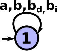
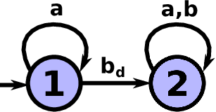
Attack functions and for the system defined in Example I.1 and were encoded in automata and depicted in Fig. 2. Automaton encodes the all-out strategy for this example. Although the all-out strategy is a nondeterministic strategy since the attacker can try all possible combinations of attacks, its automaton representation is a deterministic automaton. Only one state is necessary to encode the all-out strategy. Automaton encodes a one sensor reading deletion attack strategy.
II-C Controlled system under sensor deception attack
The attacker in the controlled system induces a new controlled language. Referring to Fig. 3, , and together effectively generate a new supervisor for the system .

To characterize the interaction of attacker with the system and supervisor realization , we must modify the behavior of and such that it takes into account possible modifications of . We use the method in [14], where and are augmented with attack actions providing an attacked system and an attacked supervisor .
Definition II.2.
Given and , we define the attacked plant as: where and .
Similarly to the construction of , we can modify the behavior of to reflect the modifications made by an attacker on the communication channel.
Definition II.3.
Given and , we define the attacked supervisor as: where
We assume that the supervisor “ignores” insertions of controllable events that are not enabled by the current control action at state . This assumption is specified by the second condition in the definition of . Namely, the insertion made by the attacker is ineffective at this state. In some sense, this means that the supervisor “knows” that this controllable event has to be an insertion performed by the attacker, since it is not an enabled event.
Based on , and , we define the closed-loop language of the attacked system to be , where is the standard parallel composition operator [21]. Recall that the transition function of is complete with respect to and for any then . Therefore, the attacker is incapable of disabling events of .
Example II.3.
We return to our running example. Figure 4 depicts the attacked system , the attacked supervisor , and the supervised attacked system , where is the all-out attack strategy shown in Fig. 2(2(a)). Note that state is reachable in the supervised attacked system.


Remark II.1.
Even though the attack function is nondeterministic, the language generated by the attacked system is uniquely defined, i.e., . In [11], the nondeterministic attack function defined therein generates maximal and minimal attacked languages. Similar to the problem encountered in [23], the maximal language possibly contains strings that the supervised plant cannot generate while the minimal does not define all possible strings that this controlled plant generates. This issue does not arise in our context. Our language definition also differs from the one in [12]. Even though an attacker could have a string of insertions to send to the supervisor, it does so by sending one event at the time. On the other hand in [12], the attacker sends the entire string modification to the supervisor.
II-D Robustness against deception attacks
We investigate the problem of synthesizing a supervisor robust against the attack strategy . We assume that the plant contains a set of critical states defined as ; these states are unsafe in the sense that they are states where physical damage to the plant might occur. Although damage is defined in relation to the set , it could be generalized in relation to any regular language by state space refinement.
Definition II.4.
Supervisor is robust (against sensor deception attacks) with respect to , and , if for any then .
The definition of robustness is dependent on the attack strategy . Recall that the all-out strategy encompasses all other attack strategies [2]. Therefore, a supervisor that is robust against the all-out strategy is robust against any other [14].
Problem II.1 (Synthesis of Robust Supervisor).
Given , and an attack strategy , synthesize a robust supervisor , if one exists, with respect to , and .
We are asking that the robust supervisor should prevent the plant from reaching a critical state regardless of the fact that it might receive inaccurate information. In other words, the supervisor will react to every event that it receives, but since it was designed to be robust to , the insertions and deletions that performs will never cause to reach . This will be guaranteed by the solution procedure presented in the next section.
III Meta-Supervisor problem
In this section, we present our approach to solve Problem II.1. We briefly explain the idea of our approach. Figure 5 shows the connection of the problem formulation space (left box) and the solution space (right box). The connection between these two spaces is given by the arrows that cross the two boxes. These arrows are labeled by results provided in this section.
In the left box of Fig. 5, we have the problem formulation space where the supervisor is unknown. Based on , , and , we construct a meta-system, called , in a space where all supervisors are defined. This construction is given in Definition III.5. The meta-system is part of the proposed solution space and it is represented in the right box of Fig. 5.
Although all supervisors are defined in , which is shown by Proposition III.1, we are only interested in robust supervisors. In order to obtain robust supervisors, we use techniques of partially observed supervisory control theory [19, 20] in the meta-system. The structure is obtained via Definition III.7 and it contains all robust supervisors against sensor deception attacks on .
Finally, to return to our problem formulation space, we extract one supervisor, if one exists, from . Such extraction is given by Algorithm 1.

III-A Definition
Inspired by the techniques of two-player reachability games, we construct an arena as it is constructed in these games. In the arena, player 1 represents the supervisor while player 2 represents the adversarial environment. The arena exhaustively captures the game between the supervisor and the environment, where the supervisor selects control decisions () and the environment executes events (). In the arena, player 1’s transitions record a control decision made by the supervisor. On the other hand, player 2’s transitions represent actions of the plant or actions of the attacker . Formally, the arena is defined as follows.
Definition III.5.
Given plant and attack function , we define the arena as 4-tuple:
| (4) |
where,
- •
is the set of states where the supervisor issues a control decision. Its states have the form of , where is the estimate of the states (as it is executed by the plant) of and is the attacker’s state. For convenience we define the projection operators for ;
- •
is the set of states where the adversarial environment issues a decision. Its states have the form , where and are defined as in states, is the last control decision made by the supervisor, and is related to inserted events. The event is equal to if the last transition was , otherwise it is equal to . We use the same projection operators for states in for ;
- •
and are respectively the actions/decisions of player 1 and player 2;
- •
is built as follows: for any and
(5) - •
is built as follows for any :
Let :
Let :
- •
is the initial S-state: .
We explain the definition of the transition functions and in detail. The definition of is simple and it defines a transition from player 1 to player 2, which records a control decision made by the supervisor, and it updates ’s state estimate according to this decision. On the other hand, is more complex since player 2 has two types of transitions.
The first type is transitions from player 2 to player 1 which characterizes the visible decision made by the environment and is related to events in . These transitions are defined in Eq. (III.5), and they are illustrated in Fig. 6. In Fig. 6(6(a)), an event that is feasible in from some state in is selected; thus, both the state estimate and the attacker’s state are updated. In Fig 6(6(b)), is reached after an insertion since ; thus, ’s state estimate and the attacker’s state remain unchanged.


Transitions from player 2 to itself characterize invisible, from the supervisor’s perspective, decisions. They are only defined for events in . These transitions are defined by Eqs. (III.5-III.5). An attacker can insert any event in , as long as is allowed in the current attacker’s state. The inserted events are not going to be seen by the supervisor, as only the attacker knows it decided to insert the event. Insertions will be seen by the supervisor as genuine events. But represents here (in the context of the game arena) the intention of the attacker to insert. Equation (III.5) (depicted in Fig. 7(7(a))) is the unobservable part, where an insertion decision was selected and the attacker’s state and the fourth component of are updated. The observable part is shown by Fig. 6(6(b)). In the case of a deleted event, from the supervisor’s perspective, it is seen as an event as well. That is, the supervisor cannot change its control decision when the attacker deletes an event, as shown in Fig. 7(7(b)).


Remark 1: The elements of and are defined such that they incorporate the “sufficient information” (in the sense of information state in system theory) that each player needs to make its respective decision. Equations (5-III.5) guarantee by construction that the updates of the information states are consistent with the plant dynamics and the actions of the attacker. Overall, the arena constructed thereby captures the possible attacks and all possible supervisors in a finite structure. We prove both results later on.
Example III.4.
We return to our illustrative example to show results on the construction of the arena. We construct for the system , and depicted in Fig. 2(2(a)). Since we construct for the all-out attack strategy, we can omit the attacker state. The arena has a total of states.Figure 8 illustrates arena constructed with respect to and . We can observe the encoding of insertion and deletion in this arena. For example, at state the transition goes to state and then transition takes state to state .

For convenience, we extend the definition of based on a given control decision. Namely, we define a transition function that always start and end in states. This notation simplifies walks in .
Definition III.6.
We define the function as:
| (17) |
The function can be recursively extended for strings given a sequence of control decisions , i.e., .
III-B Properties
For a fixed supervisor and attacker , we obtain the language which contains the possible string executions in the attacked system, e.g., strings of events in . Given a string , we can find the state estimate of after execution of , i.e., the state estimate of under supervision of and attack strategy . Formally, this state estimate is
| (18) |
In the construction of , we allow the attacker to insert events that are not allowed by the current control decision (see Eq. (III.5)). Therefore, given a supervisor , we need to define its control decisions for all , differing from the usual definition only for . For this reason, we extend the function to be a complete function in .
for and . Intuitively, extends by simply ignoring the events that are not defined in . The function is extended to as is extended. Lastly, we define the control decision of for any as:
| (21) |
Based on and , we show that the arena computes the same state estimates based on the supervisor and attacker as the ones computed based on . This result is shown in Proposition III.1 and its proof is in Appendix B.
Proposition III.1.
Given a system , a supervisor , an attack function and arena , then for any , we have that
| (22) | ||||
| (23) | ||||
| (24) | ||||
where and .
Recall that in the left box of Fig. 5 the supervisor is unknown. Equation (22) tells us that the arena captures all possible interactions between any supervisor and attack function with the plant . It captures all possible interactions since Proposition III.1 is true regardless of the supervisor and of the attack function . This is one of the main benefits of constructing the arena . It defines a space where all supervisors and attacker actions based on for the plant exist.
Moreover, Eqs. (23-24) says that the arena correctly captures the interaction between the attacker, supervisor and plant. Equation (23) computes ’s state estimate of based on the modified string and the control decisions taken by along the observed string. These estimates capture an agent that has full knowledge of the modification on the string and the decisions taken by . On the other hand, Eq. (24) establishes the correct state of the attacker in the construction of .
The arena has, in worst-case, -states and -states given that . Consequently, the worst-case running time of the construction of the arena is since . We can construct starting from its initial state and performing a breadth-first search based on equations and .
III-C Solution of the Meta-Control problem
Our approach to solve Problem II.1 is to consider the above-constructed arena as the uncontrolled system in a meta-control problem, which is posed as a supervisory control problem for a partially-observed discrete event system, as originally considered in [18]. For that reason, we will refer to as the meta-system. As will become clear in the following discussion, this supervisory control approach naturally captures our synthesis objectives, and moreover supervisory control theory provides a complete characterization of the solution. Such a methodology was previously used in [24, 25] for instance; however, in these works the meta-control problem is a control problem under full observation. The same situation does not apply in our case, where events in are unobservable (from the supervisor’s perspective).
To formally pose the meta-control problem, we need a specification for the meta-system. In fact, the specification emerges from the corresponding specification in Problem II.1, which states that the controlled system should never reach any state in . The same specification is to be enforced in , where the state estimate of represents the reachable states of . Thus, the specification for the meta-control problem is that the meta-controlled system should never reach any state such that .
The next step in the meta-control problem formulation is to specify the controllable and observable events in the meta-system . We already mentioned that all are unobservable events. In fact, they are the only unobservable events in since they are moves of the attacker that the supervisor does not directly observe. In regard to the controllable events, the supervisor makes decisions in order to react to the decisions made by the environment. Therefore, the events in are controllable, while those in are uncontrollable. Note that, we explicitly exclude the control decision composed only of uncontrollable events as a meta-controllable event; the supervisor should always be able to at least enable the uncontrollable events, otherwise it would not be admissible. In this way, the supervisor can always issue at least one control decision, i.e., enable all uncontrollable plant events. We are now able to formulate the meta-control problem.
Definition III.7.
Given constructed with respect to and , with events , as the set of controllable events and as the set of unobservable events. Let be the specification automaton, where 22 2 We use superscripts to differentiate the different arena structures, e.g., , , etc.. Calculate the supremal controllable and normal sublanguage of the language of trim with respect to the language of , and let this supremal sublanguage be generated by the solution-arena denoted by .
Note that all controllable events in the meta-control problem are also observable, i.e., . Therefore, the controllability and observability conditions are equivalent to the controllability and normality conditions. Hence, in this case, the supremal controllable and observable sublanguage exists and is equal to the supremal controllable and normal sublanguage; see, e.g., §3.7.5 in [21]. As consequence a supremal and unique solution of the meta-control problem exists. This solution is the language generated by the solution-arena .
The state structure of will depend on the algorithm used to compute the supremal controllable and normal sublanguage of trim. One example of the structure of is provided.
Example III.5.
We return to our running example. Based on , we obtain using an integrated (for controllability and normality) iterative algorithm to compute the supremal controllable and normal sublanguage that is based on preprocessing the input automata to satisfy simultaneously a strict sub-automaton [21] condition and a State Partition Automaton [26] condition. As part of the algorithm, one needs to refine so that its observer is a state partition automaton (using algorithm in [26]), i.e., to compute , where is the observer operation with respect to [21]. The resulting is depicted in Fig. 9. Each state in is a tuple, where the first component is a state in and the second component is a state in , where and .

Regardless of the algorithm to obtain , it has a structure with -like states and -like states, since it accepts a sublanguage of trim. Namely, it has states where only control decisions are allowed ( states) and states where only transitions with events in are defined ( states). Thus, we can use the functions previously defined for in .
Remark III.2.
The worst-case running time to obtain the supremal controllable and normal sublanguage is exponential in product of the number of states of the system and the specification [27]. Therefore, the worst-case running time to obtain the is .
The way is constructed is such that it embeds the set of all supervisors for the original plant . Therefore, the uniqueness of the language generated by sup and the fact that it is the supremal solution of the meta-control problem means that the structure sup embeds a family of supervisors , where the controlled behavior generated by each member of that family does not reach any state in . Moreover, since is constructed taking into account the attack function , this family of supervisors is robust with respect to . This leads us to the following result. Its proof is in Appendix B.
Theorem III.1.
A supervisor is a robust supervisor with respect to if and only if , where and .
Corollary III.1.
if and only if there does not exist any robust supervisor with respect to attacker .
Theorem III.1 states that a supervisor is robust if and only if it is embedded in . Next, Corollary III.1 gives a necessary and sufficient condition for the existence of a solution for Problem II.1. Given that there exists a robust supervisor, we provide an algorithm33 3 There are different manners for a designer to extract a robust supervisor. to extract a supervisor that solves Problem II.1. First, we define function as we defined .
Definition III.8.
Let the function be defined as:
| (25) |
Algorithm 1 starts at the initial state of sup and performs a Depth First Search by selecting the largest control decisions at each state that it visits. By largest, we mean that it selects a control decision that is not a subset of any other control decision defined at state , as described by line . Note that, it is possible to have more than two decisions that satisfy this condition. In this case, the algorithm selects one of the possible decisions in a nondeterministic manner. The algorithm terminates since is finite. Moreover, the algorithm only traverses player states, where the control decisions are defined.
Remark III.3.
The worst-case running time of Algorithm 1 is linear in the number of state of . For this reason, the running time of the entire synthesis procedure is exponential in the number of states of . Since the number of states of is exponential in the number of states of , the overall worst-case running time is double exponential in the number of states of , which is one exponential order smaller than in [12] and one exponential order higher than in [14], two references that were reviewed in Section I.


IV Selecting supervisors in the robust arena
Algorithm 1 provides one way of extracting robust supervisors from . As we explained before, it selects maximal control decisions in the states that the algorithm visits. Example III.6 shows that this extraction does not provide specific information about the language generated by supervised system once a supervisor is selected, other than the fact that we are choosing a locally maximal control decision. While supervisor in Fig. 10(10(a)) generates a live language, supervisor in Fig. 10(10(b)) is blocking. Nonetheless, the space defined in provides maximum flexibility in extracting different supervisors since all robust supervisors are embedded in . The methods in [11, 12, 14] do not provide the flexibility of since they exploit algorithms of Supervisory Control Theory where only one supervisor can be obtained at a time. In fact, when explicit comparisons can be made, the supervisors obtained by their methods are embedded in the corresponding .
Another benefit of the construction of is the ability to exploit results in the area of turn-based two-player graph-games. Results from these areas can be leveraged to study different manners of extracting robust supervisors, e.g., to study quantitative versions of the robust supervisor problem under some cost model [28, 29, 30].
We provide an example of a supervisor extraction algorithm based on a quantitative measure. First, we define a measure over the supervised system , i.e., over the states of the automaton . Let the set be the set of states in that can reach a deadlock state via an unobservable string. We define to be a reward function for any and as:
| (26) |
The reward function punishes states from where the system might deadlock. Based on the reward function , we define the following total reward for the supervised system .
| (27) |
We can generalize Algorithm 1 to incorporate this quantitative measure such that it extracts a supervisor from that maximizes the measure . In our running example, this new method extracts supervisor . Further, we can assume that the attacker tries to minimize in this extraction method. In this scenario, we would pose a problem in order to select a supervisor from . We leave these extensions for future work.
V Robot Motion Planning Example
We developed a tool44 4 Our software tool is available at: URL. URL will be included upon final acceptance of the paper. to automatically construct , as in Definition III.5, and to compute . Moreover, Algorithm 1 is also implemented in our tool. Our evaluation was done on a Linux machine with 2.2GHz CPU and 16GB memory.
We consider a robot moving in a possibly hostile environment. The robot is assumed to have four different movement modes that are modeled as controllable and observable events. The robot moves freely in the workspace shown in Fig. 11(11(a)). Its initial state is the blue cell denoted as and the red cells are considered to be obstacles. Moreover, the shaded region is assumed to be hostile and the sensor readings of the robot could be under attack. This uncontrolled system is modeled by the automaton depicted in Fig. 11(11(b)). We want to design a robust supervisor that enforces the following properties: (1) the robot must avoid the obstacles; (2) the robot can always access states and .


The set of compromised events is since we consider that the sensor readings in the shaded area might be under attack. First, we construct the arena considering the all-out attack strategy. The number of states in is states. The state space explosion is due to the number of control decisions: there are possible control decisions.
After constructing , we obtain as described in Definition III.7. To compute the supremal controllable and normal sublanguage, we used the algorithm described in Example III.5. The number of states in is states. Note that has more states than . The larger state space in is due to necessary preprocessing done by the iterative algorithm for the computation of the supremal controllable and normal sublaguage.
Finally, any supervisor selected from is robust against the all-out attack strategy, i.e., it satisfies property (1). Therefore, we must select a supervisor that satisfies property (2). For this reason, we modify Algorithm 1 to extract a supervisor from such that property (2) is satisfied. This supervisor is depicted in Fig. 12.

VI Conclusion
We have considered a class of problems in cyber-security where sensor readings in a feedback control system may be manipulated by a malicious attacker. By formulating the problem at the supervisory control layer of a cyber-physical system, we were able to leverage techniques from games on automata under partial information and from supervisory control of partially-observed discrete event systems to develop a solution methodology to prevent damage to the system when some sensor readings may be edited by the attacker. Our problem formulation is parameterized by an attacker strategy over a set of compromised events. In this manner, synthesis of robust supervisors against sensor deception attack strategies is considered, e.g., bounded attack strategies, replacement attack strategies, etc. Moreover, if there is no prior information about the attacker strategy, then we consider the general all-out attack strategy. A supervisor robust against the all-out attack strategy is robust against any other sensor deception attack strategy.
The space defined in provides maximum flexibility in extracting different supervisors since all robust supervisors are embedded in . As discussed in Section IV, it would be interesting to investigate methods to extract supervisors from sup in order to satisfy additional constraints, such as optimality with respect to some quantitative criterion [29, 28]. Finally, identifying ways to reduce the state space of the arena by exploiting a suitable notion of state equivalence is another important research direction.
Appendix A Attack function encoding
In Section II, we assume that the automaton that encodes an attack function has a transition function complete with respect to and for any then . To encode any attack function as an automaton, this assumption does not need to be satisfied. However, this means that the attacker might “block” the controlled system if it receives an unexpected event executed by the plant, i.e., is undefined.
Based on the above assumption, we relax the completeness assumption of in order to encode any attack function as an automaton. Namely, the partial transition function of must satisfy one of the following conditions for any :
- (1)
and ; or
- (2)
is not defined and ;
Condition (2) allows attack strategies where event insertion is faster than the plant executes events. Note that condition (2) violates controllability since it temporarily blocks the plant from executing events. The practicality of this assumption will depend on the plant’s response time, i.e., this attack condition is application dependent. Condition (1) remains unchanged, i.e., the attacker does not block the plant in states that satisfy this condition.
Appendix B Proofs
Proposition III.1
Proof.
The result is proved by induction on the length of the string .
Before we start the induction proof, we state two important results. First, we define in the same manner as , but the control decisions of are defined over . It can be shown by induction that the following equality holds for any :
| (28) |
Intuitively, Eq. (28) follows since is a copy or with insertion and deletions events added based on .
Second, the function can also be computed recursively as follows for and :
| (29) |
defines the unobservable events of . Then, only supervisor disables events in to be executed in since is defined over . For this reason, Eq. B is equivalent to Eq. III-B.
Induction basis: .
We have that is well defined since is complete with respect to . It also follows that since and . We have that .
| (30) | ||||
| (31) | ||||
| (32) | ||||
| (33) | ||||
| (34) |
Induction hypothesis: , and for all and .
Induction step: Let , , and . The induction hypothesis gives us , , and . Let .
Since then it follows that . Moreover, it follows that by construction of .
For equality of Eq. (23), we divide the event into three cases.
First, . Then, Based on the construction of , we have that .
| (35) | ||||
| (36) | ||||
| (37) | ||||
| (38) | ||||
| (39) |
Let, . Based on the construction of , we have that .
| (40) | ||||
| (41) | ||||
| (42) | ||||
| (43) | ||||
| (44) |
Lastly, . Based on the construction of , we have that .
| (45) | ||||
| (46) | ||||
| (47) | ||||
| (48) | ||||
| (49) |
This concludes our proof. ∎
Theorem III.1
Proof.
We start with the only if part. Let be a robust supervisor. Proposition III.1 guarantees that is defined for any and for any attack function representation . To analyze the meta-system , we have to define some notation for it.
We are analyzing as a meta-system, namely as an automaton. The function is a the combination of the functions and . Let be the event set of , the observable event set, the controllable event set. Moreover, the function projects strings in to strings in . Intuitively, for any the function returns the string that is observed by the supervisor.
We construct the language recursively as:
- 1.
- 2.
,
- 3.
The language is by construction controllable w.r.t. and ; we show that is normal w.r.t. and . The result is shown by contradiction. Assume that is not normal, then there exist shortest and s.t. . In the construction of , player 2 is not constrained, meaning that the shortest strings that belong to end with an event in (control decisions). For this reason, and . It implies that and . By the definition of , . This contradicts our assumption.
It is also true that , otherwise would not be a robust supervisor. Intuitively, the actions made by player 2 are not constrained in the construction of . This guarantees that embeds all actions of attacker . The actions of player 1 are constrained based on and . is robust and changing any of its control actions for any string by will preserve robustness since for any .
Definition III.7 defines to be the supremal controllable and normal sublanguage of w.r.t. and . Since and it is controllable and normal, then . Therefore, holds for all .
For the if part, the result follows from the construction of , and the properties of . ∎
Acknowledgment
It is a pleasure to acknowledge many useful discussions with Loïc Hélouët in the preparation of this paper. The authors are also grateful to the reviewers for their insightful comments.
References
- [1] D. Thorsley and D. Teneketzis, “Intrusion detection in controlled discrete event systems,” in Proceedings of the 45th IEEE Conference on Decision and Control, Dec 2006, pp. 6047–6054.
- [2] L. K. Carvalho, Y.-C. Wu, R. Kwong, and S. Lafortune, “Detection and mitigation of classes of attacks in supervisory control systems,” Automatica, vol. 97, pp. 121 – 133, 2018.
- [3] P. M. Lima, M. V. S. Alves, L. K. Carvalho, and M. V. Moreira, “Security against communication network attacks of cyber-physical systems,” Journal of Control, Automation and Electrical Systems, vol. 30, no. 1, pp. 125–135, Feb 2019.
- [4] F. Lin, “Robust and adaptive supervisory control of discrete event systems,” IEEE Transactions on Automatic Control, vol. 38, no. 12, pp. 1848–1852, Dec 1993.
- [5] J. Cury and B. Krogh, “Robustness of supervisors for discrete-event systems,” IEEE Transactions on Automatic Control, vol. 44, no. 2, pp. 376–379, 1999.
- [6] S. Xu and R. Kumar, “Discrete event control under nondeterministic partial observation,” in 2009 IEEE International Conference on Automation Science and Engineering, Aug 2009, pp. 127–132.
- [7] S. Takai, “Maximizing robustness of supervisors for partially observed discrete event systems,” Automatica, vol. 40, no. 3, pp. 531 – 535, 2004.
- [8] K. Rohloff, “Bounded sensor failure tolerant supervisory control,” in 11th IFAC International Workshop on Discrete Event Systems, October 2012, pp. 272 – 277.
- [9] M. V. S. Alves, J. C. Basilio, A. E. C. da Cunha, L. K. Carvalho, and M. V. Moreira, “Robust supervisory control against intermittent loss of observations,” in 12th IFAC International Workshop on Discrete Event Systems, May 2014, pp. 294 – 299.
- [10] F. Lin, “Control of networked discrete event systems: Dealing with communication delays and losses,” SIAM Journal on Control and Optimization, vol. 52, no. 2, pp. 1276–1298, 2014.
- [11] M. Wakaiki, P. Tabuada, and J. P. Hespanha, “Supervisory control of discrete-event systems under attacks,” Dynamic Games and Applications, Sep 2018.
- [12] R. Su, “Supervisor synthesis to thwart cyber attack with bounded sensor reading alterations,” Automatica, vol. 94, pp. 35 – 44, 2018.
- [13] L. Lin, Y. Zhu, and R. Su, “Towards bounded synthesis of resilient supervisors,” in 2019 IEEE 58th Conference on Decision and Control (CDC), 2019, pp. 7659–7664.
- [14] R. Meira-Góes, H. Marchand, and S. Lafortune, “Towards resilient supervisors against sensor deception attacks,” in 2019 IEEE 58th Annual Conference on Decision and Control (CDC), Dec 2019.
- [15] Y. Wang and M. Pajic, “Attack-resilient supervisory control with intermittently secure communication,” in 2019 IEEE 58th Conference on Decision and Control (CDC), 2019, pp. 2015–2020.
- [16] R. Meira-Góes, E. Kang, R. H. Kwong, and S. Lafortune, “Synthesis of sensor deception attacks at the supervisory layer of cyber–physical systems,” Automatica, vol. 121, p. 109172, 2020.
- [17] P. J. Ramadge and W. M. Wonham, “Supervisory control of a class of discrete event processes,” SIAM Journal on Control and Optimization, vol. 25, no. 1, pp. 206–230, Jan. 1987.
- [18] F. Lin and W. Wonham, “On observability of discrete-event systems,” Information Sciences, vol. 44, no. 3, pp. 173 – 198, 1988.
- [19] R. Cieslak, C. Desclaux, A. S. Fawaz, and P. Varaiya, “Supervisory control of discrete-event processes with partial observations,” IEEE Transactions on Automatic Control, vol. 33, no. 3, pp. 249–260, March 1988.
- [20] H. Cho and S. I. Marcus, “On supremal languages of classes of sublanguages that arise in supervisor synthesis problems with partial observation,” Mathematics of Control, Signals and Systems, vol. 2, no. 1, pp. 47–69, 1989.
- [21] C. G. Cassandras and S. Lafortune, Introduction to Discrete Event Systems. Secaucus, NJ, USA: Springer-Verlag New York, Inc., 2008.
- [22] P. M. Lima, M. V. Alves, L. K. Carvalho, and M. V. Moreira, “Security against network attacks in supervisory control systems,” in 20th IFAC World Congress, 2017, pp. 12 333 – 12 338.
- [23] S. Shu and F. Lin, “Supervisor synthesis for networked discrete event systems with communication delays,” IEEE Transactions on Automatic Control, vol. 60, no. 8, pp. 2183–2188, Aug 2015.
- [24] X. Yin and S. Lafortune, “A uniform approach for synthesizing property-enforcing supervisors for partially-observed discrete-event systems,” IEEE Transactions on Automatic Control, vol. 61, no. 8, pp. 2140–2154, Aug 2016.
- [25] Y. C. Wu and S. Lafortune, “Synthesis of optimal insertion functions for opacity enforcement,” IEEE Transactions on Automatic Control, vol. 61, no. 3, pp. 571–584, March 2016.
- [26] G. Jirásková and T. Masopust, “On properties and state complexity of deterministic state-partition automata,” in Proc. of 7th International Conference on Theoretical Computer Science (IFIP TCS), ser. LNCS, J. C. M. Baeten, T. Ball, and F. S. de Boer, Eds., vol. 7604. Springer, 2012, pp. 164–178.
- [27] R. Brandt, V. Garg, R. Kumar, F. Lin, S. Marcus, and W. Wonham, “Formulas for calculating supremal controllable and normal sublanguages,” Systems and Control Letters, vol. 15, no. 2, pp. 111 – 117, 1990.
- [28] F. Cassez, J. Dubreil, and H. Marchand, “Synthesis of opaque systems with static and dynamic masks,” Formal Methods in System Design, vol. 40, no. 1, pp. 88–115, 2012.
- [29] Y. Ji, X. Yin, and S. Lafortune, “Mean payoff supervisory control under partial observation,” in 2018 IEEE Conference on Decision and Control (CDC), Dec 2018, pp. 3981–3987.
- [30] R. Meira-Góes, R. Kwong, and S. Lafortune, “Synthesis of sensor deception attacks for systems modeled as probabilistic automata,” in 2019 American Control Conference (ACC), July 2019.