跳到论文正文
W Papers独立论文阅读器 arXiv:2012.12869 论文正文 计算阅读时间 · 0%
引用这篇论文根据当前论文元数据生成,正式投稿前建议核对。


License: arXiv.org perpetual non-exclusive license
arXiv:2012.12869v2 [math.SG] 21 Mar 2022

3D Convex Contact Forms And The Ruelle Invariant

J. Chaidez Address: Department of Mathematics
University of California at Berkeley
Berkeley, CA
94720
USA
Email address: jchaidez@berkeley.edu
and O. Edtmair Address: Department of Mathematics
University of California at Berkeley
Berkeley, CA
94720
USA
Email address: oliver_edtmair@berkeley.edu
Abstract.

Let X⊂R4X\subset\mathbb{R}^{4} be a convex domain with smooth boundary YY. We use a relation between the extrinsic curvature of YY and the Ruelle invariant of the Reeb flow on YY to prove that there are constants C>c>0C>c>0 independent of YY such that

c≤ru⁡(Y)⋅sys⁡(Y)1/2≤Cc\leq\operatorname{ru}(Y)\cdot\operatorname{sys}(Y)^{1/2}\leq C

Here sys⁡(Y)\operatorname{sys}(Y) is the systolic ratio of YY, i.e. the square of the minimal period of a closed Reeb orbit of YY divided by twice the volume of XX, and ru⁡(Y)\operatorname{ru}(Y) is the volume-normalized Ruelle invariant. We then construct dynamically convex contact forms on S3S^{3} that violate this bound using methods of Abbondandolo-Bramham-Hryniewicz-Salomão. These are the first examples of dynamically convex contact 33-spheres that are not strictly contactomorphic to a convex boundary YY.

1. Introduction

A contact manifold (Y,ξ)(Y,\xi) is an odd dimensional manifold equipped with a hyperplane field ξ⊂T​Y\xi\subset TY, called the contact structure, that is the kernel of a 11-form α\alpha such that

ker⁡(d​α)⊂T​Y​ is rank 1andα|ker⁡(d​α)>0\ker(d\alpha)\subset TY\text{ is rank 1}\qquad\text{and}\qquad\alpha|_{\ker(d\alpha)}>0

A 11-form satisfying this condition is called a contact form on (Y,ξ)(Y,\xi). Every contact form comes equipped with a natural Reeb vector field RR, defined by

α⁡(R)=1ιR​d​α=0\alpha(R)=1\qquad\iota_{R}d\alpha=0

Note that the Reeb vector-field preserves the 11-form α\alpha and the natural volume form α∧d​αn−1\alpha\wedge d\alpha^{n-1}, where dim⁡(Y)=2​n−1\operatorname{dim}\left({Y}\right)=2n-1. The dynamical properties of Reeb vector fields (e.g. the existence of closed orbits and their properties) are the subject of immense interest in symplectic geometry and dynamical systems.

Contact manifolds arise naturally as hypersurfaces in symplectic manifolds satisfying a certain stability condition. In fact, Weinstein introduced contact manifolds in [27] inspired by the following prototypical example of this phenomenon, due to Rabinowitz [21].

Example 1.1.

We say that a domain X⊂R2​nX\subset\mathbb{R}^{2n} with smooth boundary YY is star-shaped if

0∈int⁡(X)and∂r is transverse to ​Y0\in\operatorname{int}(X)\qquad\text{and}\qquad\partial_{r}\text{ is transverse to }Y

Let ω\omega and ZZ denote the standard symplectic form and Liouville vector field on R2​n\mathbb{R}^{2n}. That is

(1.1) ω=∑i=1ndxi∧dyiZ=12∑ixi∂xi+yi∂yi=12r∂r\omega=\sum_{i=1}^{n}dx_{i}\wedge dy_{i}\qquad Z=\frac{1}{2}\sum_{i}x_{i}\partial_{x_{i}}+y_{i}\partial_{y_{i}}=\frac{1}{2}r\partial_{r}

Then the restriction λ|Y\lambda|_{Y} of the Liouville 11-form λ=ιZ​ω\lambda=\iota_{Z}\omega is a contact form.

Example 1.2.

The standard contact structure ξ\xi on S2​n−1⊂R2​nS^{2n-1}\subset\mathbb{R}^{2n} is given by ξ=ker⁡(λ|S2​n−1)\xi=\ker(\lambda|_{S^{2n-1}}).

Every contact form on the standard contact sphere arises as the pullback of λ\lambda via a map to a star-shaped boundary YY. Indeed, if α=f⋅λ|S2​n−1\alpha=f\cdot\lambda|_{S^{2n-1}} for f>0f>0 is a contact form for ξ\xi, then

α=ϕ∗​λwhereϕ⁡(θ)=(f​(θ)1/2,θ)in radial coordinates ​(0,∞)r×Sθ2​n−1\alpha=\phi^{*}\lambda\qquad\text{where}\qquad\phi(\theta)=(f(\theta)^{1/2},\theta)\quad\text{in radial coordinates }(0,\infty)_{r}\times S^{2n-1}_{\theta}

Moreover, every star-shaped boundary YY admits such a map from the sphere. Thus, from the perspective of contact geometry, the study of star-shaped boundaries is equivalent to the study of contact forms on the standard contact sphere.

1.1. Convexity

In this paper, we are primarily interested in studying contact forms arising as boundaries of convex domains.

Definition 1.3.

A contact form α\alpha on S2​n−1S^{2n-1} is convex if there is a convex star-shaped domain X⊂R2​nX\subset\mathbb{R}^{2n} with boundary YY and a strict contactomorphism (S3,α)≃(Y,λ|Y)(S^{3},\alpha)\simeq(Y,\lambda|_{Y}).

In contrast to the star-shaped case, not every contact form on S2​n−1S^{2n-1} is convex, and the Reeb flows of convex contact forms possess many special dynamical properties, both proven and conjectural.

In [26], Viterbo proposed a particularly remarkable systolic inequality for Reeb flows on convex boundaries. To state it, let (Y,α)(Y,\alpha) be a closed contact manifold with contact form of dimension 2​n−12n-1, and recall that the volume vol⁡(Y,α)\operatorname{vol}\left({Y,\alpha}\right) and systolic ratio sys⁡(Y,α)\operatorname{sys}(Y,\alpha) are given by

(1.2) vol⁡(Y,α)=∫Yα∧d​αn−1andsys⁡(Y,α)=min⁡{period T of an orbit}nvol⁡(Y,α)\operatorname{vol}\left({Y,\alpha}\right)=\int_{Y}\alpha\wedge d\alpha^{n-1}\qquad\text{and}\qquad\operatorname{sys}(Y,\alpha)=\frac{\operatorname{min}\left\{{\text{period $T$ of an orbit}}\right\}^{n}}{\operatorname{vol}\left({Y,\alpha}\right)}

Note that if YY is the boundary of a star-shaped domain X⊂R2​nX\subset\mathbb{R}^{2n}, then the contact volume of (Y,λ|Y)(Y,\lambda|_{Y}) is related to the volume of XX via vol⁡(Y,λ|Y)=n!​vol⁡(X)\operatorname{vol}\left({Y,\lambda|_{Y}}\right)=n!\operatorname{vol}\left({X}\right). The weak Viterbo conjecture that originally appeared in [26] can be stated as follows.

Conjecture 1.4.

[26] Let α\alpha be a convex contact form on S2​n−1S^{2n-1}. Then the systolic ratio is bounded by 11.

sys⁡(S2​n−1,α)≤1\operatorname{sys}(S^{2n-1},\alpha)\leq 1

There is also a strong Viterbo conjecture (c.f. [14]), stating that all normalized symplectic capacities are equal on convex domains. For other special properties of convex domains, see [15, 26].

Despite the plethora of distinctive properties that convex contact forms possess, a characterization of convexity entirely in terms of contact geometry has remained elusive.

Problem 1.5.

Give an intrinsic characterization of convexity that does not reference a map to R2​n\mathbb{R}^{2n}.

1.2. Dynamical Convexity

In the seminal paper [15], Hofer-Wysocki-Zehnder provided a candidate answer to Problem 1.5.

Definition 1.6 (Def. 3.6, [15]).

A contact form α\alpha on S3S^{3} is dynamically convex if the Conley-Zehnder index CZ⁡(γ)\operatorname{CZ}(\gamma) of any closed Reeb orbit γ\gamma is greater than or equal to 33.

The Conley-Zehnder index of a Reeb orbit plays the role of the Morse index in symplectic field theory and other types of Floer homology (see §2.2 for a review). Thus, on a naive level, dynamical convexity may be viewed as a type of “Floer-theoretic” convexity. If XX is a convex domain whose boundary YY has positive definite second fundamental form, then YY is dynamically convex [15, Thm 3.7]. Note that this condition is open and dense among convex boundaries.

In [15], Hofer-Wysocki-Zehnder proved that the Reeb flow of a dynamically convex contact form admits a surface of section. In the decades since, dynamical convexity has been used as a key hypothesis in many significant works on Reeb dynamics and other topics in contact and symplectic geometry. See the papers of Hryniewicz [16], Zhou [28, 29], Abreu-Macarini [3, 4], Ginzburg-Gürel [11], Fraunfelder-Van Koert [9] and Hutchings-Nelson [18] for just a few examples. However, the following question has remained stubbornly open (c.f. [9, p. 5]).

Question 1.7.

Is every dynamically convex contact form on S3S^{3} also convex?

The recent paper [1] of Abbondandolo-Bramham-Hryniewicz-Salomão (ABHS) has suggested that the answer to Question 1.7 should be no. They construct dynamically convex contact forms on S3S^{3} with systolic ratio close to 22. There is substantial evidence for the weak Viterbo conjecture (cf. [6]), and so these contact forms are likely not convex. However, this was not proven in [1].

Even more recently, Ginzburg-Macarini [12] addressed a version of Question 1.7 in higher dimensions that incorporates the assumption of symmetry under the antipod map S2​n−1→S2​n−1S^{2n-1}\to S^{2n-1}. Their work did not address the general case of Question 1.7.

1.3. Main Result

The main purpose of this paper is to resolve Question 1.7.

Theorem 1.8.

There exist dynamically convex contact forms α\alpha on S3S^{3} that are not convex.

Theorem 1.8 is an immediate application of Proposition 1.9 and 1.12, which we will now describe.

1.4. Ruelle Bound

For our first result, recall that any closed contact 33-manifold (Y,ξ)(Y,\xi) with contact form α\alpha that satisfies c1​(ξ)=0c_{1}(\xi)=0 and H1​(Y,Z)=0H^{1}(Y;\mathbb{Z})=0 has an associated Ruelle invariant [23]

Ru⁡(Y,α)∈R\operatorname{Ru}(Y,\alpha)\in\mathbb{R}

Roughly speaking, the Ruelle invariant is the integral over YY of a time-averaged rotation number that measures the degree to which different Reeb trajectories twist counter-clockwise around each other (see §2.4 for a detailed review). Our result is stated most elegantly using the quantity

ru⁡(Y,α)=Ru⁡(Y,α)vol⁡(Y,α)1/2\operatorname{ru}(Y,\alpha)=\frac{\operatorname{Ru}(Y,\alpha)}{\operatorname{vol}\left({Y,\alpha}\right)^{1/2}}

This Ruelle ratio is invariant under scaling of the contact form, unlike the Ruelle invariant itself.

In recent work [17] motivated by embedded contact homology, Hutchings investigated the Ruelle invariant of toric domains in C2\mathbb{C}^{2}. In that paper, the Ruelle invariant of the standard ellipsoid E=E⁡(a,b)⊂C2E=E(a,b)\subset\mathbb{C}^{2} with symplectic radii 0<a≤b0<a\leq b (see §3.1) was computed as

(1.3) Ru⁡(E)=a+b\operatorname{Ru}(E)=a+b

The systolic ratio sys⁡(E)\operatorname{sys}(E) and contact volume vol⁡(∂E,λ|∂E)\operatorname{vol}(\partial E,\lambda|_{\partial E}) are well-known to be a/ba/b and a​bab respectively. Thus we have the following relation between the systolic and Ruelle ratios.

ru(E)=sys(E)1/2+sys(E)−1/2and thus1<ru(E)⋅sys(E)1/2=sys(E)+1≤2\operatorname{ru}(E)=\operatorname{sys}(E)^{1/2}+\operatorname{sys}(E)^{-1/2}\quad\text{and thus}\quad 1<\operatorname{ru}(E)\cdot\operatorname{sys}(E)^{1/2}=\operatorname{sys}(E)+1\leq 2

Our first result may be viewed as a generalization of the estimate on the right to arbitrary convex contact forms on S3S^{3}.

Proposition 1.9 (Prop 3.1).

There are constants C>c>0C>c>0 such that, for any convex contact form α\alpha on S3S^{3}, the following inequality holds.

(1.4) c≤ru⁡(S3,α)⋅sys⁡(S3,α)1/2≤Cc\leq\operatorname{ru}(S^{3},\alpha)\cdot\operatorname{sys}(S^{3},\alpha)^{1/2}\leq C

Note that a result of Viterbo [26, Thm 5.1] states that there exists a constant γ2\gamma_{2} such that sys⁡(S3,α)≤γ2\operatorname{sys}(S^{3},\alpha)\leq\gamma_{2} for any convex contact form. Thus, Proposition 1.9 also implies that

Corollary 1.10.

There is a constant c>0c>0 such that, for any convex contact form α\alpha on S3S^{3}, we have

(1.5) c≤ru⁡(S3,α)c\leq\operatorname{ru}(S^{3},\alpha)

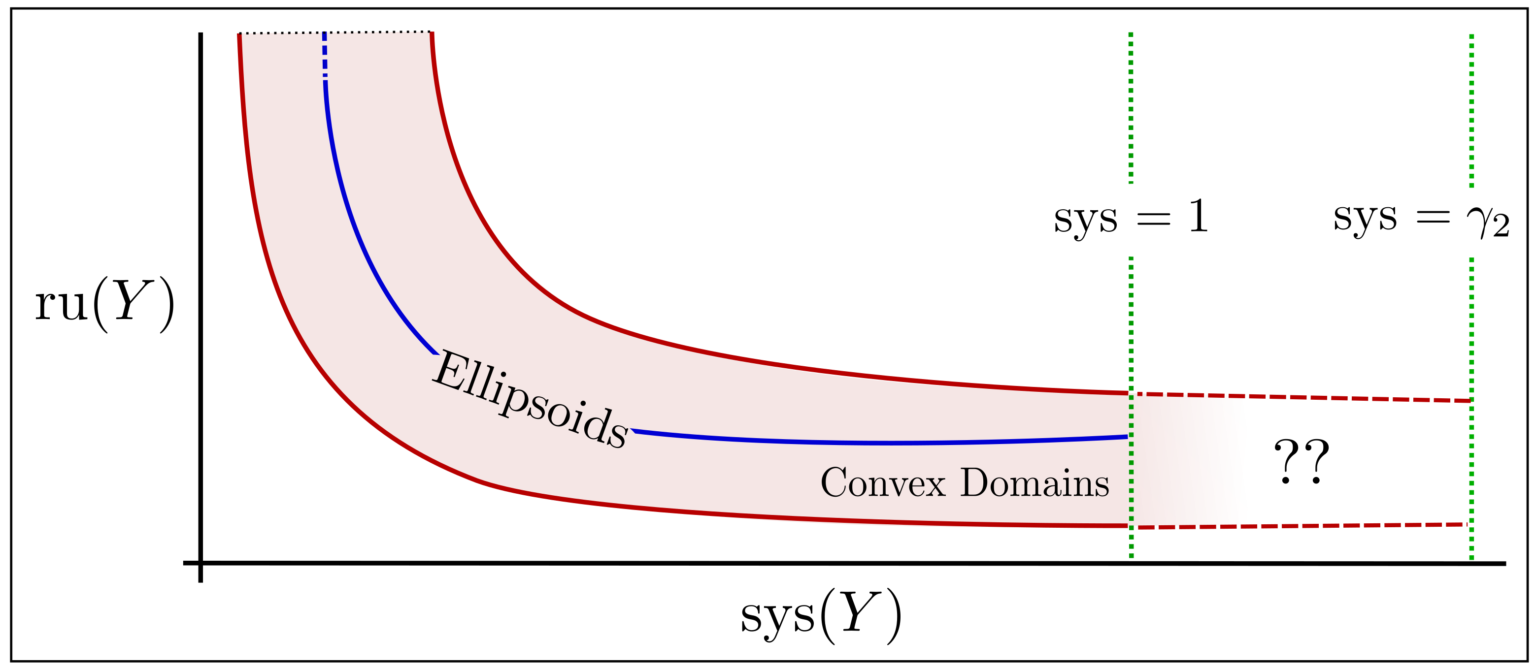
It is notable that, even for ellipsoids, the systolic ratio can be arbitrarily close to 00 and the Ruelle ratio can be arbitrarily close to ∞\infty. We have included a helpful visualization of Proposition 1.9 in the sys−ru\operatorname{sys}-\operatorname{ru} plane in Figure 1.

Figure 1. A plot of the region of the sys−ru\operatorname{sys}-\operatorname{ru} plane containing convex contact forms, depicted in light red. The blue arc is the region occupied by ellipsoids, and the green lines represent the sys=1\operatorname{sys}=1 bound and the sys=γ2\operatorname{sys}=\gamma_{2} bound. The Viterbo conjecture states that the region of convex domains with systolic ratio larger than 11 is empty, and so it is partially shaded in this figure.
Refer to caption

Let us explain the idea of the proof of Proposition 1.9. First, as explained above, the result holds for ellipsoids. By applying John’s ellipsoid theorem [19], we can sandwich a given convex domain XX between an ellipsoid EE and its scaling 4⋅E4\cdot E. After applying an affine symplectomorphism to XX and EE, we may assume that EE is standard. That is

E⁡(a,b)⊂X⊂4⋅E⁡(a,b)E(a,b)\subset X\subset 4\cdot E(a,b)

Note that this symplectomorphism does not change the Ruelle invariant (see §3.1). Now note that the minimum length of a closed orbit is monotonic under inclusion of convex domains, since it coincides the the Ekeland-Hofer-Zehnder capacity in the convex setting (cf. [7]). Applying this and the monotonicity of volume, we find that

(1.6) a​b2≤vol⁡(X)≤28⋅a​b2and2−8⋅ab≤sys⁡(Y)≤28⋅ab\frac{ab}{2}\leq\operatorname{vol}\left({X}\right)\leq 2^{8}\cdot\frac{ab}{2}\qquad\text{and}\qquad 2^{-8}\cdot\frac{a}{b}\leq\operatorname{sys}(Y)\leq 2^{8}\cdot\frac{a}{b}

If the Ruelle invariant were also monotonic, then one could immediately acquire Proposition 1.9 from (1.6) and (1.3). Unfortunately, this is not evidently the case.

The resolution of this issue comes from a beautiful formula (Proposition 3.10) relating the second fundmantal form and local rotation of the Reeb flow on a contact hypersurface YY in R4\mathbb{R}^{4}. This is due originally to Ragazzo-Salomão [22], albeit in different language from this paper. Using this relation (§3.2), we derive estimates for the Ruelle invariant in terms of diameter, area and total mean curvature. By standard convexity theory (i.e. the theory of mixed volumes), these quantities are monotonic under inclusion of convex domains. This allows us to compare the Ruelle invariant of XX to that of its sandwiching ellipsoids, and thus prove the result.

Remark 1.11 (Enhancing Prop 1.9).

In future work, we plan to investigate optimal constants cc and CC for Proposition 1.9, and to generalize the result to higher dimensions.

1.5. A Counterexample

In order to prove Theorem 1.8 using Proposition 1.9, we construct dynamically convex contact forms that violate both sides of the estimate (1.5). This is the subject of our second new result.

Proposition 1.12 (Prop 4.1).

For every ϵ>0\epsilon>0, there exists a dynamically convex contact form α\alpha on S3S^{3} satisfying

vol⁡(S3,α)=1sys⁡(S3,α)≥1−ϵRu⁡(S3,α)≤ϵ\operatorname{vol}\left({S^{3},\alpha}\right)=1\qquad\operatorname{sys}(S^{3},\alpha)\geq 1-\epsilon\qquad\operatorname{Ru}(S^{3},\alpha)\leq\epsilon

and there exists a dynamically convex contact form β\beta on S3S^{3} satisfying

vol⁡(S3,β)=1sys⁡(S3,β)≥1−ϵRu⁡(S3,β)≥ϵ−1\operatorname{vol}\left({S^{3},\beta}\right)=1\qquad\operatorname{sys}(S^{3},\beta)\geq 1-\epsilon\qquad\operatorname{Ru}(S^{3},\beta)\geq\epsilon^{-1}

The construction of these examples follows the open book methods of Abbondandolo-Bramham-Hryniewicz-Salomão in [2, 1]. Namely, we develop a detailed correspondence between the properties of a Hamiltonian disk map ϕ:D→D\phi:\mathbb{D}\to\mathbb{D} and the properties of a contact form α\alpha on S3S^{3} constructed using ϕ\phi via the open book construction (see Proposition 4.8). This includes a new formula relating the Ruelle invariant of ϕ\phi in the sense of [23] and the Ruelle invariant of (S3,α)(S^{3},\alpha). We then construct Hamiltonian disk maps ϕ\phi with all of the appropriate properties to produce dynamically convex contact forms on S3S^{3} satisfying the conditions in Proposition 1.12.

Let us briefly outline the construction in the small Ruelle case, as the large Ruelle case is similar. The special Hamiltonian map ϕ\phi is acquired by composing two maps ϕH\phi^{H} and ϕG\phi^{G}. The map ϕH\phi^{H} is a counter-clockwise rotation by angle 2​π​(1+1/n)2\pi(1+1/n) for large nn. The map ϕG\phi^{G} is compactly supported on a disjoint union UU of disks DD, and rotates (most of) each disk DD clockwise about its center by angle slightly less than 4​π4\pi. See Figure 2 for an illustration of this map.

Figure 2. The map ϕ=ϕG∘ϕH\phi=\phi^{G}\circ\phi^{H} for n=4n=4. Here ϕH\phi^{H} rotates D\mathbb{D} counter-clockwise by 90 degrees and ϕG\phi^{G} twists each disk DD by roughly 720 degrees clockwise.
Refer to caption

Applying Proposition 4.8, we can show that the volume and Ruelle invariant of (S3,α)(S^{3},\alpha) are (up to negligible error) proportional to the following quantities.

vol⁡(S3,α)∼π2−2​∑Darea⁡(D)2Ru⁡(S3,α)∼2​π−2​∑Darea⁡(D)\operatorname{vol}\left({S^{3},\alpha}\right)\sim\pi^{2}-2\sum_{D}\operatorname{area}(D)^{2}\qquad\operatorname{Ru}(S^{3},\alpha)\sim 2\pi-2\sum_{D}\operatorname{area}(D)

By choosing UU to fill most of D\mathbb{D} and choosing all of the disks in UU to be very small, we can make the Ruelle invariant very small relative to the volume. This process preserves the minimal action of a closed orbit (up to a small error) and dynamical convexity, producing the desired small Ruelle invariant example.

Remark 1.13.

Our examples do not coincide with the ABHS examples in [1]. However, we believe that improvements of Proposition 1.12 may make our analysis applicable to those examples.

Remark 1.14.

In general, it is possible for the Ruelle invariant of a Reeb flow on S3S^{3} to be negative. However, Proposition 1.9 implies (via the lower bound) that the Ruelle invariant of a convex contact form is always positive. In fact, this is a much simpler property to prove than Proposition 1.9 itself, using similar methods. However, we were not able to push the construction in §4 to yield a dynamically convex contact form with non-positive Ruelle invariant.

Outline

This concludes the introduction §1. The rest of the paper is organized as follows.

In §2, we cover basic preliminaries needed in later sections: the rotation number (§2.1), the Conley-Zehnder index (§2.2), invariants of Reeb orbits (§2.3) and the Ruelle invariant (§2.4).

In §3, we prove Proposition 1.9. We start by discussing the curvature-rotation formula and some consequences (§3.2). We then derive a lower bound for a relevant curvature integral (§3.3). We conclude by proving the main bound (§3.4).

In §4, we prove Proposition 1.12. We first discuss general preliminaries on Hamiltonian disk maps (§4.1), open books (§4.2) and radial Hamiltonians (§4.3). We then construct a Hamiltonian flow on the disk (§4.4) before concluding with the main proof (§4.5).

Acknowledgements

We are deeply indepted to Alberto Abbondandolo, Umberto Hryniewicz and Michael Hutchings, who explained a number of the ideas and arguments in §2 to JC in various discussions and private communications. We would also like thank the anonymous referees for suggesting that we include counter-examples in §4 that violate the upper bound in Proposition 3.1. JC was supported by the NSF Graduate Research Fellowship under Grant No. 1752814.

2. Rotation Numbers And Ruelle Invariant

In this section, we review some preliminaries on rotation numbers, Conley-Zehnder indices and the Ruelle invariant, which we will need in later parts of the paper.

Remark 2.1.

The rotation number, also known as the homogeneous Maslov quasimorphism, and the Conley-Zehnder index were originally introduced by Gelfand-Lidskii [10] albeit using different terminology. For a more contemporary perspective, see Salamon-Zehnder [24].

2.1. Rotation Number

Consider the universal cover Sp~​(2)\widetilde{\operatorname{Sp}}(2) of the symplectic group Sp⁡(2)\operatorname{Sp}(2). We will view a group element Φ\Phi as a homotopy class of paths with fixed endpoints

Φ:[0,1]→Sp⁡(2)withΦ⁡(0)=Id\Phi:[0,1]\to\operatorname{Sp}(2)\quad\text{with}\quad\Phi(0)=\operatorname{Id}

Recall that a quasimorphism q:G→Rq:G\to\mathbb{R} from a group GG to the real line is a map such that there exists a C>0C>0 such that

(2.1) |q⁡(g​h)−q⁡(g)−q⁡(h)|<Cfor all ​g,h∈G|q(gh)-q(g)-q(h)|<C\qquad\text{for all }g,h\in G

A quasimorphism is homogeneous if q⁡(gk)=k⋅q⁡(g)q(g^{k})=k\cdot q(g) for any g∈Gg\in G. Finally, two quasimorphisms qq and q′q^{\prime} are called equivalent if the function |q−q′||q-q^{\prime}| on GG is bounded. Note that any quasimorphism is equivalent to a unique homogeneous one.

The universal cover of the symplectic group possesses a canonical homogeneous quasimorphism, due to the following result of Salamon-Ben Simon [25].

Theorem 2.2 ([25], Thm 1).

There exists a unique homogeneous quasimorphism

ρ:Sp~​(2)→R\rho:\widetilde{\operatorname{Sp}}(2)\to\mathbb{R}

that restricts to the following homomorphism ρ:U~​(1)→R\rho:\widetilde{\operatorname{U}}(1)\to\mathbb{R} on the universal cover of U⁡(1)\operatorname{U}(1).

(2.2) ρ⁡(γ)=Lon the path ​γ:[0,1]→U⁡(1)​ with ​γ​(t)=exp⁡(2​π​i​L​t)\rho(\gamma)=L\qquad\text{on the path }\gamma:[0,1]\to\operatorname{U}(1)\text{ with }\gamma(t)=\exp(2\pi iLt)
Definition 2.3.

The rotation number ρ:Sp~​(2)→R\rho:\widetilde{\operatorname{Sp}}(2)\to\mathbb{R} is the quasimorphism in Theorem 2.2.

The rotation number is often characterized more explicitly in the literature as a lift of a map to the circle. More precisely, it is characterized as the unique lift

(2.3) σ~:Sp~​(2)→Rofσ:Sp⁡(2)→S1such thatσ~​(Id)=0\widetilde{\sigma}:\widetilde{\operatorname{Sp}}(2)\to\mathbb{R}\qquad\text{of}\qquad\sigma:\operatorname{Sp}(2)\to S^{1}\qquad\text{such that}\qquad\widetilde{\sigma}(\operatorname{Id})=0

via the covering map R→S1⊂C\mathbb{R}\rightarrow S^{1}\subset\mathbb{C} given by θ↦e2​π​i​θ\theta\mapsto e^{2\pi i\theta}. Here σ\sigma is defined as follows. Let Φ∈Sp⁡(2)\Phi\in\operatorname{Sp}(2) have real eigenvalues λ,λ−1\lambda,\lambda^{-1} and let Ψ∈Sp⁡(2)\Psi\in\operatorname{Sp}(2) have complex (unit) eigenvalues ζ,ζ¯\zeta,\overline{\zeta} with Im⁡ζ>0\operatorname{Im}\zeta>0. Also fix an arbitrary v∈R2∖0v\in\mathbb{R}^{2}\setminus 0, identified with an element of C\mathbb{C} in the usual way. Then

(2.4) σ⁡(Φ)={0 if ​λ>01/2 if ​λ<0andσ⁡(Ψ)={ζ if ​⟨i​v,Φ​v⟩>0ζ¯ if ​⟨i​v,Φ​v⟩<0\sigma(\Phi)=\left\{\begin{array}[]{cc}\vskip 4.0pt0&\text{ if }\lambda>0\\ 1/2&\text{ if }\lambda<0\\ \end{array}\right.\quad\text{and}\quad\sigma(\Psi)=\left\{\begin{array}[]{cc}\vskip 4.0pt\zeta&\text{ if }\langle iv,\Phi v\rangle>0\\ \overline{\zeta}&\text{ if }\langle iv,\Phi v\rangle<0\\ \end{array}\right.

Here i​viv denotes multiplication of vv by i∈Ci\in\mathbb{C}, i.e. the rotation of vv by 90 degrees counterclockwise. All of the elements of Sp⁡(2)\operatorname{Sp}(2) fall into one of the two categories above, and so σ\sigma is determined everywhere by (2.4).

Lemma 2.4.

The rotation number ρ:Sp~​(2)→R\rho:\widetilde{\operatorname{Sp}}(2)\to\mathbb{R} is the lift of σ:Sp⁡(2)→R/Z\sigma:\operatorname{Sp}(2)\to\mathbb{R}/\mathbb{Z} with ρ⁡(Id)=0\rho(\operatorname{Id})=0.

Proof.

We verify the properties in Theorem 2.2. The lift σ~\widetilde{\sigma} is a quasimorphism by Lemmas 2.6 and 2.7 below. Also note that since eigenvalues and the sign of ⟨i​v,Φ​v⟩\langle iv,\Phi v\rangle are invariant under conjugation, σ\sigma is as well.

To check that σ~\widetilde{\sigma} is homogeneous, note that if Φ\Phi has real eigenvalues of sign s=±1s=\pm 1, then σ⁡(Φk)=12​(1−sk)=k​smod1\sigma(\Phi^{k})=\frac{1}{2}(1-s^{k})=ks\mod 1. On the otherhand, if Φ\Phi has complex unit eigenvalues ζ,ζ¯\zeta,\bar{\zeta} for Re⁡(ζ)>0\operatorname{Re}(\zeta)>0, then it is conjugate to a rotation exp⁡(2​π​i​θ)∈U⁡(1)⊂Sp⁡(2)\exp(2\pi i\theta)\in U(1)\subset\operatorname{Sp}(2) on C≃R2\mathbb{C}\simeq\mathbb{R}^{2} and thus

σ⁡(Φk)=σ⁡(exp⁡(2​π​i​k​θ))=k​θmod1\sigma(\Phi^{k})=\sigma(\exp(2\pi ik\theta))=k\theta\mod 1

Thus σ⁡(Φk)=k⋅σ⁡(Φ)mod1\sigma(\Phi^{k})=k\cdot\sigma(\Phi)\mod 1 and the lift satisifes σ~​(Φk)=k​σ~​(Φ)\widetilde{\sigma}(\Phi^{k})=k\widetilde{\sigma}(\Phi). Finally, if γ:[0,1]→Sp⁡(2)\gamma:[0,1]\to\operatorname{Sp}(2) is given by γ⁡(t)=exp⁡(2​π​i​L​t)\gamma(t)=\exp(2\pi iLt) then

σ∘γ:[0,1]→R/Zis given byσ∘γ⁡(t)=L​tmod1∈R/Z\sigma\circ\gamma:[0,1]\to\mathbb{R}/\mathbb{Z}\quad\text{is given by}\quad\sigma\circ\gamma(t)=Lt\mod 1\in\mathbb{R}/\mathbb{Z}

This implies that the lift is t↦L​tt\mapsto Lt, so that σ~​(γ)=L\widetilde{\sigma}(\gamma)=L. This proves the needed criteria. ∎

We will also need to utilize several inhomogeneous versions of the rotation number depending on a choice of unit vector. These are defined a follows.

Definition 2.5.

The rotation number ρs:Sp~​(2)→R\rho_{s}:\widetilde{\operatorname{Sp}}(2)\to\mathbb{R} relative to s∈S1s\in S^{1} is the unique lift of the map

σs:Sp⁡(2)→S1Φ↦|Φ​s|−1⋅Φ​s∈S1⊂R2\sigma_{s}:\operatorname{Sp}(2)\to S^{1}\qquad\Phi\mapsto|\Phi s|^{-1}\cdot\Phi s\in S^{1}\subset\mathbb{R}^{2}

via the covering map R→S1⊂C\mathbb{R}\to S^{1}\subset\mathbb{C} given by θ↦e2​π​i​θ⋅s\theta\mapsto e^{2\pi i\theta}\cdot s such that ρs​(Id)=0\rho_{s}(\operatorname{Id})=0. Here Φ​s\Phi s denotes the application of the matrix Φ∈Sp⁡(2)\Phi\in\operatorname{Sp}(2) to the unit vector s∈S1s\in S^{1}.

The rotation numbers relative to s∈S1s\in S^{1} and the lift of σ\sigma all have bounded difference from one another. Precisely, we have the following lemma.

Lemma 2.6.

The maps ρs:Sp~​(2)→R\rho_{s}:\widetilde{\operatorname{Sp}}(2)\to\mathbb{R} and the lift σ~:Sp~​(2)→R\widetilde{\sigma}:\widetilde{\operatorname{Sp}}(2)\to\mathbb{R} of σ\sigma have bounded difference. More precisely, we have the following bounds.

(2.5) |ρs−σ~|≤1and|ρs−ρt|≤1for any pair ​s,t∈S1|\rho_{s}-\widetilde{\sigma}|\leq 1\qquad\text{and}\qquad|\rho_{s}-\rho_{t}|\leq 1\qquad\text{for any pair }s,t\in S^{1}
Proof.

First, assume that Φ:[0,1]→Sp⁡(2)\Phi:[0,1]\to\operatorname{Sp}(2) is a path such that Φ⁡(t)\Phi(t) has no negative real eigenvalues for any t∈[0,1]t\in[0,1]. Then

σ∘Φ⁡(t)≠1/2andσs∘Φ⁡(t)≠−s∈S1 for any ​s∈S1​ and ​t∈[0,1]\sigma\circ\Phi(t)\neq 1/2\qquad\text{and}\qquad\sigma_{s}\circ\Phi(t)\neq-s\in S^{1}\qquad\text{ for any }s\in S^{1}\text{ and }t\in[0,1]

It follows that the relevant lifts of σ∘Φ\sigma\circ\Phi and σs∘Φ\sigma_{s}\circ\Phi to maps [0,1]→R[0,1]\to\mathbb{R} remain in the interval (−1/2,1/2)(-1/2,1/2) for all tt. Thus

σ~(Φ)∈(−1/2,1/2)andρs(Φ)∈(−1/2,1/2)\widetilde{\sigma}(\Phi)\in(-1/2,1/2)\qquad\text{and}\qquad\rho_{s}(\Phi)\in(-1/2,1/2)

This clearly implies (2.5) since Φ⁡(t)\Phi(t) does not have any negative eigenvalues. Since σ\sigma induces an isomorphism π1​(Sp⁡(2))→π1​(S1)\pi_{1}(\operatorname{Sp}(2))\to\pi_{1}(S^{1}), we know that for any pair Φ,Φ′∈Sp~​(2)\Phi,\Phi^{\prime}\in\widetilde{\operatorname{Sp}}(2) with the same projection to Sp⁡(2)\operatorname{Sp}(2)

σ~​(Φ)=σ~​(Φ′)impliesΦ=Φ′\widetilde{\sigma}(\Phi)=\widetilde{\sigma}(\Phi^{\prime})\qquad\text{implies}\qquad\Phi=\Phi^{\prime}

In particular, the above analysis extends to any Φ\Phi with σ~(Φ)∈(−1/2,1/2)\widetilde{\sigma}(\Phi)\in(-1/2,1/2). In the general case, note that the path γ:[0,1]→S1\gamma:[0,1]\to S^{1} given by γ⁡(t)=exp⁡(π​i⋅k​t)\gamma(t)=\exp(\pi i\cdot kt) for an integer k∈Zk\in\mathbb{Z} satisfies

σ~​(γ)=ρs​(γ)=k/2σ~​(Φ​γ)=σ~​(Φ)+σ~​(γ)ρs​(Φ​γ)=ρs​(Φ)+ρs​(γ)\widetilde{\sigma}(\gamma)=\rho_{s}(\gamma)=k/2\qquad\widetilde{\sigma}(\Phi\gamma)=\widetilde{\sigma}(\Phi)+\widetilde{\sigma}(\gamma)\qquad\rho_{s}(\Phi\gamma)=\rho_{s}(\Phi)+\rho_{s}(\gamma)

Any path Ψ\Psi can be decomposed (up to homotopy) as Φ​γ\Phi\gamma where γ\gamma is as above and Φ:[0,1]→Sp⁡(2)\Phi:[0,1]\to\operatorname{Sp}(2) is a path with σ~(Φ)∈(−1/2,1/2)\widetilde{\sigma}(\Phi)\in(-1/2,1/2). This reduces to the special case. ∎

This can be used to demonstrate that ρs\rho_{s} is a quasimorphism. As noted in the proof of Lemma 2.4, this implies that σ~\widetilde{\sigma} is a quasimorphism as well.

Lemma 2.7.

The map ρs:Sp~​(2)→R\rho_{s}:\widetilde{\operatorname{Sp}}(2)\to\mathbb{R} is a quasimorphism for any s∈S1s\in S^{1}. In fact, we have

(2.6) |ρs​(Ψ​Φ)−ρs​(Ψ)−ρs​(Φ)|≤1for anys∈S1|\rho_{s}(\Psi\Phi)-\rho_{s}(\Psi)-\rho_{s}(\Phi)|\leq 1\qquad\text{for any}\qquad s\in S^{1}
Proof.

Let Φ:[0,1]→Sp⁡(2)\Phi:[0,1]\to\operatorname{Sp}(2) and Ψ:[0,1]→Sp⁡(2)\Psi:[0,1]\to\operatorname{Sp}(2) be two elements of Sp~​(2)\widetilde{\operatorname{Sp}}(2) viewed as paths in Sp⁡(2)\operatorname{Sp}(2). Consider the product Ψ​Φ\Psi\Phi in the universal cover of Sp⁡(2)\operatorname{Sp}(2), represented by the path

Φ⁡(2​t)​ for ​t∈[0,1/2]andΨ⁡(2​t−1)​Φ​(1)​ for ​t∈[1/2,1]\Phi(2t)\text{ for }t\in[0,1/2]\qquad\text{and}\qquad\Psi(2t-1)\Phi(1)\text{ for }t\in[1/2,1]

By examining the path σs∘Ψ​Φ:[0,1]→S1\sigma_{s}\circ\Psi\Phi:[0,1]\to S^{1} and the lift to R\mathbb{R}, we deduce the following property.

(2.7) ρs​(Ψ​Φ)=ρΦ⁡(s)​(Ψ)+ρs​(Φ)\rho_{s}(\Psi\Phi)=\rho_{\Phi(s)}(\Psi)+\rho_{s}(\Phi)

Here Φ⁡(s)\Phi(s) is shorthand for the unit vector Φ⁡(1)​s/|Φ⁡(1)​s|\Phi(1)s/|\Phi(1)s|. Applying Lemma 2.6, we have

|ρs​(Ψ​Φ)−ρs​(Ψ)−ρs​(Φ)|≤|ρΦ⁡(s)​(Ψ)−ρs​(Ψ)|≤1|\rho_{s}(\Psi\Phi)-\rho_{s}(\Psi)-\rho_{s}(\Phi)|\leq|\rho_{\Phi(s)}(\Psi)-\rho_{s}(\Psi)|\leq 1

This proves the quasimorphism property.∎

2.2. Conley-Zehnder Index

Let Sp⋆⁡(2)⊂Sp⁡(2)\operatorname{Sp}_{\star}(2)\subset\operatorname{Sp}(2) denote the subset of elements Φ∈Sp⁡(2)\Phi\in\operatorname{Sp}(2) such that Φ−Id\Phi-\operatorname{Id} is invertible, and let Sp~⋆​(2)\widetilde{\operatorname{Sp}}_{\star}(2) be the inverse image of Sp⋆⁡(2)\operatorname{Sp}_{\star}(2) under π:Sp~​(2)→Sp⁡(2)\pi:\widetilde{\operatorname{Sp}}(2)\to\operatorname{Sp}(2).

The Conley-Zehnder index is a natural integer invariant of paths in Sp⋆⁡(2)\operatorname{Sp}_{\star}(2), denoted as follows.

CZ:Sp~⋆​(2)→Z\operatorname{CZ}:\widetilde{\operatorname{Sp}}_{\star}(2)\to\mathbb{Z}

This invariant was introduce in [10] (also see [24]). We will use the following formula as our definition throughout this paper.

(2.8) CZ⁡(Φ)=⌊ρ⁡(Φ)⌋+⌈ρ⁡(Φ)⌉\operatorname{CZ}(\Phi)=\lfloor\rho(\Phi)\rfloor+\lceil\rho(\Phi)\rceil

There are several inequivalent ways to extend the Conley-Zehnder index to the entire symplectic group. We will follow [15, §3] and [1, §2.2], and use the following extension.

Convention 2.8.

In this paper, the Conley-Zehnder index CZ:Sp~​(2)→Z\operatorname{CZ}:\widetilde{\operatorname{Sp}}(2)\to\mathbb{Z} will be the maximal lower semi-continuous extension of the ordinary Conley-Zehnder index.

The extension in Convention 2.8 can be bounded from below in terms of the rotation number.

Lemma 2.9.

Let Φ∈Sp~​(2)\Phi\in\widetilde{\operatorname{Sp}}(2). Then

(2.9) CZ⁡(Φ)≥2⋅⌈ρ⁡(Φ)⌉−1\operatorname{CZ}(\Phi)\geq 2\cdot\lceil\rho(\Phi)\rceil-1
Proof.

For Φ∈Sp~⋆​(2)\Phi\in\widetilde{\operatorname{Sp}}_{\star}(2), (2.9) is an immediate consequence of (2.8). In the other case, note that the maximal lower semi-continuous extension is defined by the property that

CZ⁡(Φ)=lim infΨ→ΦCZ⁡(Ψ)for any ​Φ∉Sp~⋆​(2)\operatorname{CZ}(\Phi)=\liminf_{\Psi\rightarrow\Phi}\operatorname{CZ}(\Psi)\qquad\text{for any }\Phi\not\in\widetilde{\operatorname{Sp}}_{\star}(2)

Any Φ∉Sp~⋆​(2)\Phi\not\in\widetilde{\operatorname{Sp}}_{\star}(2) has eigenvalue 11, and so Lemma 2.4 implies that ρ⁡(Φ)∈Z\rho(\Phi)\in\mathbb{Z}. Since ρ\rho is continuous, we find that

CZ⁡(Φ)=lim infΨ→Φ⌊ρ⁡(Ψ)⌋+⌈ρ⁡(Ψ)⌉≥⌊ρ⁡(Φ)−1/2⌋+⌈ρ⁡(Φ)−1/2⌉=2⋅⌈ρ⁡(Φ)⌉−1\operatorname{CZ}(\Phi)=\liminf_{\Psi\rightarrow\Phi}\lfloor\rho(\Psi)\rfloor+\lceil\rho(\Psi)\rceil\geq\lfloor\rho(\Phi)-1/2\rfloor+\lceil\rho(\Phi)-1/2\rceil=2\cdot\lceil\rho(\Phi)\rceil-1

This proves the lower bound in every case. ∎

2.3. Invariants Of Reeb Orbits

Let (Y,ξ)(Y,\xi) be a closed contact 33-manifold with c1​(ξ)=0c_{1}(\xi)=0 and let α\alpha be a contact 1-form on YY.

Under this hypothesis on the Chern class, ξ\xi is isomorphic as a symplectic vector-bundle to the trivial bundle R2\mathbb{R}^{2}. A trivialization τ\tau of ξ\xi is a bundle isomorphism

τ:ξ≃R2denoted byτ⁡(y):ξy≃R2satisfyingτ​(y)∗​ω=d​α|ξ\tau:\xi\simeq\mathbb{R}^{2}\qquad\text{denoted by}\qquad\tau(y):\xi_{y}\simeq\mathbb{R}^{2}\qquad\text{satisfying}\qquad\tau(y)^{*}\omega=d\alpha|_{\xi}

Two trivializations are homotopic if they are connected by a 1-parameter family of bundle isomorphisms. Given a trivialization τ\tau, we may associate a linearized Reeb flow

(2.10) Φτ:R×Y→Sp⁡(2)given byΦτ​(T,y)=τ⁡(ϕT​(y))∘d​ϕT​(y)∘τ−1​(y)\Phi_{\tau}:\mathbb{R}\times Y\to\operatorname{Sp}(2)\qquad\text{given by}\qquad\Phi_{\tau}(T,y)=\tau(\phi_{T}(y))\circ d\phi_{T}(y)\circ\tau^{-1}(y)

Here ϕ:R×Y→Y\phi:\mathbb{R}\times Y\to Y is the Reeb flow, i.e. the flow generated by the Reeb vector field RR, and we use the notation ϕT​(y)=ϕ⁡(T,y)\phi_{T}(y)=\phi(T,y). The linearized flow lifts uniquely to a map

Φ~τ:R×Y→Sp~​(2) with Φ~τ|0×Y=Id∈Sp~​(2)\widetilde{\Phi}_{\tau}:\mathbb{R}\times Y\to\widetilde{\operatorname{Sp}}(2)\qquad\text{ with }\qquad\widetilde{\Phi}_{\tau}|_{0\times Y}=\operatorname{Id}\in\widetilde{\operatorname{Sp}}(2)

We will refer to Φ~τ\widetilde{\Phi}_{\tau} as the lifted linearized Reeb flow. Explicitly, it maps (T,y)(T,y) to the homotopy class of the path Φτ​(⋅,y)|[0,T]\Phi_{\tau}(\cdot,y)|_{[0,T]}. Note that this lift satisfies the cocyle property

(2.11) Φ~τ​(S+T,y)=Φ~τ​(T,ϕS​(y))⋅Φ~τ​(S,y)\widetilde{\Phi}_{\tau}(S+T,y)=\widetilde{\Phi}_{\tau}(T,\phi_{S}(y))\cdot\widetilde{\Phi}_{\tau}(S,y)
Definition 2.10.

Let γ:R/L​Z→Y\gamma:\mathbb{R}/L\mathbb{Z}\to Y be a closed Reeb orbit of YY. The action of γ\gamma is given by

(2.12) 𝒜⁡(γ)=∫γ∗​α=L\mathcal{A}(\gamma)=\int\gamma^{*}\alpha=L

Likewise, the rotation number and Conley-Zehnder index of γ\gamma with respect to τ\tau are given by

(2.13) ρ⁡(γ,τ):=ρ∘Φ~τ​(L,y)CZ⁡(γ,τ):=CZ⁡(Φ~τ​(L,y))where ​y=γ⁡(0)\rho(\gamma,\tau):=\rho\circ\widetilde{\Phi}_{\tau}(L,y)\qquad\operatorname{CZ}(\gamma,\tau):=\operatorname{CZ}(\widetilde{\Phi}_{\tau}(L,y))\qquad\text{where }y=\gamma(0)

These invariants depend only on the homotopy class of τ\tau, and if H1​(Y,Z)=0H^{1}(Y;\mathbb{Z})=0 (e.g. if YY is the 3-sphere) there is a unique trivialization up to homotopy. In this case, we let

(2.14) ρ⁡(γ):=ρ⁡(γ,τ)andCZ⁡(γ):=CZ⁡(γ,τ)for any τ\rho(\gamma):=\rho(\gamma,\tau)\qquad\text{and}\qquad\operatorname{CZ}(\gamma):=\operatorname{CZ}(\gamma,\tau)\qquad\text{for any $\tau$}

In §4, we will need the following easy observation, which follows immediately from Lemma 2.9 and our way of defining CZ\operatorname{CZ} (see Convention 2.8).

Lemma 2.11.

Let α\alpha be a contact form on S3S^{3} with ρ⁡(γ)>1\rho(\gamma)>1 for every closed Reeb orbit. Then α\alpha is dynamically convex.

2.4. Ruelle Invariant

Let (Y,ξ)(Y,\xi) be a closed contact 33-manifold with c1​(ξ)=0c_{1}(\xi)=0 equipped with a contact form α\alpha and a homotopy class of trivialization [τ][\tau] of ξ\xi. Here we discuss the Ruelle invariant

Ru⁡(Y,α,[τ])∈R\operatorname{Ru}(Y,\alpha,[\tau])\in\mathbb{R}

associated to the data of Y,αY,\alpha and [τ][\tau].

Remark 2.12.

This invariant was originally introduced by Ruelle in [23] for area preserving diffeomorphisms of surfaces and volume preserving flows on 3-manifolds. Variants of this construction have also appeared under different names in other settings, e.g. as the asymptotic Maslov index [8, p. 1423].

It will be helpful to describe a more general construction that subsumes that of the Ruelle invariant. For this purpose, we also fix a continuous quasimorphism

q:Sp~​(2)→Rq:\widetilde{\operatorname{Sp}}(2)\to\mathbb{R}

Pick a representative trivialization τ\tau of [τ][\tau] and let Φ~τ:R×Y→Sp~​(2)\widetilde{\Phi}_{\tau}:\mathbb{R}\times Y\to\widetilde{\operatorname{Sp}}(2) be the lifted linearized Reeb flow. We can associate a time-averaged version of qq over the space YY, as follows.

Proposition 2.13.

The 11-parameter family of functions fT:Y→Rf_{T}:Y\to\mathbb{R} given by the formula

(2.15) fT​(y):=q∘Φ~τ​(T,y)Tf_{T}(y):=\frac{q\circ\widetilde{\Phi}_{\tau}(T,y)}{T}

converges in L1​(Y,R)L^{1}(Y;\mathbb{R}) and almost everywhere to a function f⁡(α,q,τ):Y→Rf(\alpha,q,\tau):Y\to\mathbb{R} with the following properties.

  • (a)

    (Quasimorphism) If qq and rr are equivalent quasimorphisms, i.e. |q−r||q-r| is bounded, then

    f⁡(α,q,τ)=f⁡(α,r,τ)f(\alpha,q,\tau)=f(\alpha,r,\tau)
  • (b)

    (Trivialization) If σ\sigma and τ\tau are homotopic trivializations of ξ\xi, then

    f⁡(α,q,σ)=f⁡(α,q,τ)f(\alpha,q,\sigma)=f(\alpha,q,\tau)
  • (c)

    (Contact Form) The integral F⁡(α)F(\alpha) of f⁡(α,q,τ)f(\alpha,q,\tau) over YY is continuous in the C2C^{2}-topology on Ω1​(Y)\Omega^{1}(Y).

In order to prove the existence part of this result, we will need to use a verison of Kingman’s subadditivity theorem appearing in [20].

Theorem 2.14.

Let YY be a measure space and let ϕ:R×Y→Y\phi:\mathbb{R}\times Y\to Y be a flow with invariant measure μ\mu. Let gT:Y→Rg_{T}:Y\to\mathbb{R} for T∈RT\in\mathbb{R} be a family of L1​(Y,μ)L^{1}(Y,\mu) functions such that, for some constants C,D>0C,D>0, we have

gS+T≤gS+ϕS∗gT+C∫YgT⋅μ≥−D⋅T∫Y(sup0≤S≤1|gS|)⋅μ<∞g_{S+T}\leq g_{S}+\phi^{*}_{S}g_{T}+C\qquad\qquad\int_{Y}g_{T}\cdot\mu\geq-D\cdot T\qquad\qquad\int_{Y}\big(\sup_{0\leq S\leq 1}|g_{S}|\big)\cdot\mu<\infty

Then the maps gTT\frac{g_{T}}{T} converge in L1​(Y,μ)L^{1}(Y,\mu) and pointwise almost everywhere as T→∞T\to\infty.

Remark 2.15.

There is also a version of Theorem 2.14 in [20] for a discrete dynamical system, i.e a map ϕ:Y→Y\phi:Y\to Y preserving μ\mu. The statement is directly analogous to Theorem 2.14, but the last condition on the integrability of sup0≤S≤1|gS|\sup_{0\leq S\leq 1}|g_{S}| is unnecessary. We will use this version in §4.1.

Remark 2.16.

This statement is a slight variation of Theorem 4 in [20], which states the result for general sub-additive processes. Our version follows from the discussion in §1.3 of [20] for the continuous parameter space R\mathbb{R}. Note that we also weaken sub-additivity by allowing gTg_{T} to be sub-additive with respect to TT up to an overall constant factor.

Proof.

(Proposition 2.13) We prove the existence of the limit and the properties (a)-(c) separately.

Convergence. We apply Kingman’s ergodic theorem, Theorem 2.14. Fix a constant C>0C>0 for the quasimorphism qq satisfying (2.1). Let gTg_{T} denote the function on YY given by

gT:=T​fT=q∘Φ~τ​(T,−)g_{T}:=Tf_{T}=q\circ\widetilde{\Phi}_{\tau}(T,-)

Now we verify the properties in Theorem 2.14. First, due to the cocycle property (2.11) we have

(2.16) gS+T=q∘Φ~τ​(S+T,−)≤q∘Φ~τ​(S,−)+q∘Φ~τ​(T,ϕS​(−))+C=gS+ϕS∗​gT+Cg_{S+T}=q\circ\widetilde{\Phi}_{\tau}(S+T,-)\leq q\circ\widetilde{\Phi}_{\tau}(S,-)+q\circ\widetilde{\Phi}_{\tau}(T,\phi_{S}(-))+C=g_{S}+\phi^{*}_{S}g_{T}+C

We can analogously show that gS+T≥gS+ϕS∗​gT−Cg_{S+T}\geq g_{S}+\phi^{*}_{S}g_{T}-C. In particular, if T>0T>0 is a sufficiently large time with T=n+ST=n+S and S∈[0,1]S\in[0,1], then

(2.17) ∫YgT⋅α∧𝑑α≥∑k=0n−1∫Yϕk∗​g1⋅α∧𝑑α+∫Yϕn∗​gS⋅α∧𝑑α−C​T≥−A​T\int_{Y}g_{T}\cdot\alpha\wedge d\alpha\geq\sum_{k=0}^{n-1}\int_{Y}\phi^{*}_{k}g_{1}\cdot\alpha\wedge d\alpha+\int_{Y}\phi_{n}^{*}g_{S}\cdot\alpha\wedge d\alpha-CT\geq-AT

Here AA is any number larger than CC and larger than the quantity

−min⁡{∫YgS⋅α∧𝑑α:S∈[0,1]}-\operatorname{min}\left\{\int_{Y}g_{S}\cdot\alpha\wedge d\alpha\;:\;S\in[0,1]\right\}

Finally, since q∘Φ~τq\circ\widetilde{\Phi}_{\tau} is continuous on R×Y\mathbb{R}\times Y, it is clear that supT∈[0,1]⁡|fT|\operatorname{sup}_{T\in[0,1]}|f_{T}| is continuous and bounded. In particular, it is integrable. Thus gTg_{T} satisfies the criteria in Theorem 2.14, and we may conclude that gTT\frac{g_{T}}{T} converges in L1L^{1} and almost everywhere to a map

f⁡(α,q,τ)∈L1​(Y,R)f(\alpha,q,\tau)\in L^{1}(Y;\mathbb{R})

Quasimorphisms. Let qq and rr be equivalent quasimorphisms, and pick C>0C>0 such that |q−r|<C|q-r|<C everywhere. Then

‖q∘Φ~τT−r∘Φ~τT‖L1≤C⋅vol⁡(Y,α)T\|\frac{q\circ\widetilde{\Phi}_{\tau}}{T}-\frac{r\circ\widetilde{\Phi}_{\tau}}{T}\|_{L^{1}}\leq\frac{C\cdot\operatorname{vol}\left({Y,\alpha}\right)}{T}

Taking the limit as T→∞T\to\infty shows that the limiting functions f⁡(α,q,τ)f(\alpha,q,\tau) and f⁡(α,r,τ)f(\alpha,r,\tau) are equal.

Trivializations. Let σ\sigma and τ\tau be two trivializations of ξ\xi in the homotopy class [τ][\tau]. Then there is a transition map Ψ:Y→Sp⁡(2)\Psi:Y\to\operatorname{Sp}(2) given by

Ψ⁡(y):R2→R2withΨ⁡(y)=τ⁡(y)⋅σ​(y)−1\Psi(y):\mathbb{R}^{2}\to\mathbb{R}^{2}\qquad\text{with}\qquad\Psi(y)=\tau(y)\cdot\sigma(y)^{-1}

The linearized flows of σ\sigma and τ\tau are related via this transition map, by the following formula.

Φτ​(T,y)=Ψ⁡(ϕ⁡(T,y))⋅Φσ​(T,y)⋅Ψ−1​(y)\Phi_{\tau}(T,y)=\Psi(\phi(T,y))\cdot\Phi_{\sigma}(T,y)\cdot\Psi^{-1}(y)

Since σ\sigma and τ\tau are homotopic, Ψ\Psi is homotopic to a constant map. In particular, Ψ\Psi lifts to the universal cover of Sp⁡(2)\operatorname{Sp}(2). Thus we may write

Φ~τ​(T,y)=Ψ~​(ϕ⁡(T,y))⋅Φ~σ​(T,y)⋅Ψ~−1​(y)\widetilde{\Phi}_{\tau}(T,y)=\widetilde{\Psi}(\phi(T,y))\cdot\widetilde{\Phi}_{\sigma}(T,y)\cdot\widetilde{\Psi}^{-1}(y)

Here Ψ~:Y→Sp~​(2)\widetilde{\Psi}:Y\to\widetilde{\operatorname{Sp}}(2) is any lift of Ψ\Psi. The quasimorphism property of ρ\rho now implies that

‖q∘Φ~σ​(T,y)T−q∘Φ~τ​(T,y)T‖L1≤2​C+sup|q∘Ψ~|+sup|q∘Ψ~−1|T⋅vol⁡(Y,α)\|\frac{q\circ\widetilde{\Phi}_{\sigma}(T,y)}{T}-\frac{q\circ\widetilde{\Phi}_{\tau}(T,y)}{T}\|_{L^{1}}\leq\frac{2C+\sup|q\circ\widetilde{\Psi}|+\sup|q\circ\widetilde{\Psi}^{-1}|}{T}\cdot\operatorname{vol}\left({Y,\alpha}\right)

Taking the limit as T→∞T\to\infty shows that f⁡(α,q,σ)=f⁡(α,q,τ)f(\alpha,q,\sigma)=f(\alpha,q,\tau).

Contact Form. Fix a contact form α\alpha and an ϵ>0\epsilon>0. Since qq is a quasimorphism, there exists a C>0C>0 depending only on qq such that

|ρ∘Φ~τ​(n​T,y)−∑k=0n−1ρ∘Φ~τ​(T,ϕTk​(y))|≤C​n for any ​n,T>0|\rho\circ\widetilde{\Phi}_{\tau}(nT,y)-\sum_{k=0}^{n-1}\rho\circ\widetilde{\Phi}_{\tau}(T,\phi_{T}^{k}(y))|\leq Cn\qquad\text{ for any }n,T>0

We can divide by n​TnT and rewrite this estimate in terms of fTf_{T} to see that

|fn​T−1n​∑k=0n−1fT∘ϕTk|≤CT for any ​n,T>0|f_{nT}-\frac{1}{n}\sum_{k=0}^{n-1}f_{T}\circ\phi_{T}^{k}|\leq\frac{C}{T}\qquad\text{ for any }n,T>0

We can then integrate over YY and take the limit as n→∞n\to\infty to acquire

(2.18) |F⁡(α)−∫YfT⋅α∧𝑑α|=limn→∞|∫Y(fn​T−fT)⋅α∧𝑑α||F(\alpha)-\int_{Y}f_{T}\cdot\alpha\wedge d\alpha|=\lim_{n\to\infty}|\int_{Y}(f_{nT}-f_{T})\cdot\alpha\wedge d\alpha|
=limn→∞|∫Y(fn​T−1n​∑k=0n−1fT∘ϕTk)⋅α∧𝑑α|≤C⋅vol⁡(Y,α)T=\lim_{n\to\infty}|\int_{Y}(f_{nT}-\frac{1}{n}\sum_{k=0}^{n-1}f_{T}\circ\phi_{T}^{k})\cdot\alpha\wedge d\alpha|\leq\frac{C\cdot\operatorname{vol}\left({Y,\alpha}\right)}{T}

We use the fact that ϕT\phi_{T} preserves α∧d​α\alpha\wedge d\alpha in moving from the first to the second line above.

Next, fix a different contact form β\beta. Let Ψ~τ\widetilde{\Psi}_{\tau} be the lifted linearized flow for β\beta, and let

gT:Y→RwheregT​(y)=q∘Ψ~τ​(T,−)Tg_{T}:Y\to\mathbb{R}\quad\text{where}\quad g_{T}(y)=\frac{q\circ\widetilde{\Psi}_{\tau}(T,-)}{T}

Due to (2.18), we can fix a T>0T>0 such that, for all β\beta sufficiently C0C^{0}-close to α\alpha, we have

(2.19) |F⁡(α)−∫YfT⋅α∧𝑑α|<ϵ3and|F⁡(β)−∫YgT⋅β∧𝑑β|<2​C​vol⁡(Y,α)T<ϵ3|F(\alpha)-\int_{Y}f_{T}\cdot\alpha\wedge d\alpha|<\frac{\epsilon}{3}\quad\text{and}\quad|F(\beta)-\int_{Y}g_{T}\cdot\beta\wedge d\beta|<\frac{2C\operatorname{vol}\left({Y,\alpha}\right)}{T}<\frac{\epsilon}{3}

Furthermore, we may bound the integrals of fTf_{T} and gTg_{T} as follows.

(2.20) |∫YfT⋅α∧𝑑α−∫YgT⋅β∧𝑑β|≤∫Y|fT−gT|⋅α∧𝑑α+|∫YfT⋅(α∧𝑑α−β∧𝑑β)||\int_{Y}f_{T}\cdot\alpha\wedge d\alpha-\int_{Y}g_{T}\cdot\beta\wedge d\beta|\leq\int_{Y}|f_{T}-g_{T}|\cdot\alpha\wedge d\alpha+|\int_{Y}f_{T}\cdot(\alpha\wedge d\alpha-\beta\wedge d\beta)|
≤‖fT−gT‖C0​(Y)⋅vol⁡(Y,α)+‖gT‖C0​(Y)⋅|vol⁡(Y,α)−vol⁡(Y,β)|\leq\|f_{T}-g_{T}\|_{C^{0}(Y)}\cdot\operatorname{vol}\left({Y,\alpha}\right)+\|g_{T}\|_{C^{0}(Y)}\cdot|\operatorname{vol}\left({Y,\alpha}\right)-\operatorname{vol}\left({Y,\beta}\right)|

We can choose β\beta sufficiently close to α\alpha in C2​(Y)C^{2}(Y) so that Ψ~τ\widetilde{\Psi}_{\tau} is arbitrarily C0C^{0}-close to Φ~τ\widetilde{\Phi}_{\tau} on [0,T]×Y[0,T]\times Y. Since YY is compact, the image of Φ~​(T,−)\widetilde{\Phi}(T,-) is compact in Sp~​(2)\widetilde{\operatorname{Sp}}(2) for fixed time TT. Thus, since qq is continuous, gT=q∘Ψ~τ​(T,−)g_{T}=q\circ\widetilde{\Psi}_{\tau}(T,-) can also be made arbitrarily C0C^{0}-close to fT=q∘Φ~τ​(T,−)f_{T}=q\circ\widetilde{\Phi}_{\tau}(T,-). In particular, for β\beta sufficiently C2C^{2}-close to α\alpha we have

(2.21) ‖fT−gT‖C0​(Y)⋅vol⁡(Y,α)+‖gT‖C0​(Y)⋅|vol⁡(Y,α)−vol⁡(Y,β)|<ϵ3\|f_{T}-g_{T}\|_{C^{0}(Y)}\cdot\operatorname{vol}\left({Y,\alpha}\right)+\|g_{T}\|_{C^{0}(Y)}\cdot|\operatorname{vol}\left({Y,\alpha}\right)-\operatorname{vol}\left({Y,\beta}\right)|<\frac{\epsilon}{3}

Together, (2.19), (2.20) and (2.21) imply that, for β\beta sufficiently C2C^{2}-close to α\alpha, we have |F⁡(α)−F⁡(β)|<ϵ|F(\alpha)-F(\beta)|<\epsilon. This proves continuity.

This concludes the proof of the existence and properties of f⁡(α,q,τ)f(\alpha,q,\tau), and of Proposition 2.13.∎

Proposition 2.13 allows us to introduce the Ruelle invariant as an integral quantity, as follows.

Definition 2.17 (Ruelle Invariant).

The local rotation number rotτ\operatorname{rot}_{\tau} of a closed contact manifold (Y,α)(Y,\alpha) equipped with a (homotopy class of) trivialization τ\tau is the following limit in L1L^{1}.

(2.22) rotτ:Y→Rgiven byrotτ:=limT→∞ρ∘Φ~τ​(T,−)T\operatorname{rot}_{\tau}:Y\to\mathbb{R}\qquad\text{given by}\qquad\operatorname{rot}_{\tau}:=\lim_{T\to\infty}\frac{\rho\circ\widetilde{\Phi}_{\tau}(T,-)}{T}

Similarly, the Ruelle invariant Ru⁡(Y,α,τ)\operatorname{Ru}(Y,\alpha,\tau) is the integral of the local rotation number over YY, i.e.

(2.23) Ru⁡(Y,α,τ)=∫Yrotτ⋅α∧𝑑α=limT→∞1T​∫Yρ∘Φ~τ⋅α∧𝑑α\operatorname{Ru}(Y,\alpha,\tau)=\int_{Y}\operatorname{rot}_{\tau}\cdot\alpha\wedge d\alpha=\lim_{T\to\infty}\frac{1}{T}\int_{Y}\rho\circ\widetilde{\Phi}_{\tau}\cdot\alpha\wedge d\alpha

We will require an alternative expression for the Ruelle invariant in order to derive estimates later in the paper.

The Reeb flow ϕ\phi on YY preserves the contact structure, and so lifts to a flow on the total space of the contact structure ξ\xi. Since this flow is fiberwise linear, it descends to the (oriented) projectivization P​ξP\xi. A trivialization τ\tau determines an identification P​ξ≃Y×R/ZP\xi\simeq Y\times\mathbb{R}/\mathbb{Z}, and so a flow

(2.24) Φ¯:R×Y×R/Z→Y×R/Zgenerated by a vector field R¯ on Y×R/Z\bar{\Phi}:\mathbb{R}\times Y\times\mathbb{R}/\mathbb{Z}\to Y\times\mathbb{R}/\mathbb{Z}\qquad\text{generated by a vector field $\bar{R}$ on $Y\times\mathbb{R}/\mathbb{Z}$}

Let θ:Y×R/Z→R/Z\theta:Y\times\mathbb{R}/\mathbb{Z}\to\mathbb{R}/\mathbb{Z} denote the tautological projection.

Definition 2.18.

The rotation density ϱτ:Y×R/Z→R\varrho_{\tau}:Y\times\mathbb{R}/\mathbb{Z}\to\mathbb{R} is the Lie derivative

(2.25) ϱτ:=ℒR¯​(θ)\varrho_{\tau}:=\mathcal{L}_{\bar{R}}(\theta)
Lemma 2.19.

The Ruelle invariant Ru⁡(Y,α,τ)\operatorname{Ru}(Y,\alpha,\tau) is written using the rotation density ϱτ\varrho_{\tau} as

Ru⁡(Y,α,τ)=limT→∞1T​∫0T(∫YΦ¯t∗​ϱτ​(−,s)⋅α∧𝑑α)​𝑑tfor any fixed ​s∈R/Z\operatorname{Ru}(Y,\alpha,\tau)=\lim_{T\to\infty}\frac{1}{T}\int_{0}^{T}\big(\int_{Y}\bar{\Phi}_{t}^{*}\varrho_{\tau}(-,s)\cdot\alpha\wedge d\alpha\big)dt\qquad\text{for any fixed }s\in\mathbb{R}/\mathbb{Z}
Proof.

By comparing Definition 2.5 with the formula (2.24), one may verify that

σs∘Φτ​(T,y)andθ∘Φ¯​(T,y,s)−s are equal in ​R/Z\sigma_{s}\circ\Phi_{\tau}(T,y)\quad\text{and}\quad\theta\circ\bar{\Phi}(T,y,s)-s\quad\text{ are equal in }\mathbb{R}/\mathbb{Z}

Therefore, these formulas define a single map R×Y×R/Z→R/Z\mathbb{R}\times Y\times\mathbb{R}/\mathbb{Z}\to\mathbb{R}/\mathbb{Z}, admitting a unique lift to a map F:R×Y×R/Z→RF:\mathbb{R}\times Y\times\mathbb{R}/\mathbb{Z}\to\mathbb{R} that vanishes on 0×Y×R/Z0\times Y\times\mathbb{R}/\mathbb{Z}. The first formula implies that

(2.26) F⁡(T,y,s)=ρs∘Φ~τ​(T,y)F(T,y,s)=\rho_{s}\circ\widetilde{\Phi}_{\tau}(T,y)

On the other hand, let tt be the R\mathbb{R}-variable of FF and θ∘Φ¯\theta\circ\bar{\Phi}. Then the tt-derivative of FF is

d​Fd​t|T=dd​t​(θ∘Φ¯)|T=Φ¯T∗​(ℒR¯​(θ))=Φ¯T∗​ϱτ\frac{dF}{dt}|_{T}=\frac{d}{dt}(\theta\circ\bar{\Phi})|_{T}=\bar{\Phi}_{T}^{*}(\mathcal{L}_{\bar{R}}(\theta))=\bar{\Phi}_{T}^{*}\varrho_{\tau}

Integrating this identity and combining it with (2.26), we acquire the formula

(2.27) ρs∘Φ~τ​(T,y)=F⁡(T,y,s)=∫0TΦ¯t∗​ϱτ​(y,s)⋅𝑑t\rho_{s}\circ\widetilde{\Phi}_{\tau}(T,y)=F(T,y,s)=\int_{0}^{T}\bar{\Phi}_{t}^{*}\varrho_{\tau}(y,s)\cdot dt

Now, since ρs\rho_{s} and ρ\rho are equivalent by Lemma 2.6, we can apply Proposition 2.13(a) to see that

(2.28) Ru⁡(Y,α,τ)=limT→∞∫Yρs∘Φ~τ​(T,−)T⋅α∧𝑑α\operatorname{Ru}(Y,\alpha,\tau)=\lim_{T\to\infty}\int_{Y}\frac{\rho_{s}\circ\widetilde{\Phi}_{\tau}(T,-)}{T}\cdot\alpha\wedge d\alpha

We then apply (2.27) and Fubini’s theorem to see that the righthand side is given by

(2.29) limT→∞1T​∫Y(∫0TΦ¯t∗​ϱτ​(−,s)​𝑑t)​α∧𝑑α=limT→∞1T​∫0T(∫YΦ¯t∗​ϱτ​(−,s)⋅α∧𝑑α)​𝑑t\lim_{T\to\infty}\frac{1}{T}\int_{Y}\big(\int_{0}^{T}\bar{\Phi}_{t}^{*}\varrho_{\tau}(-,s)dt\big)\alpha\wedge d\alpha=\lim_{T\to\infty}\frac{1}{T}\int_{0}^{T}\big(\int_{Y}\bar{\Phi}_{t}^{*}\varrho_{\tau}(-,s)\cdot\alpha\wedge d\alpha\big)dt

This concludes the proof. ∎

3. Bounding The Ruelle Invariant

Let X⊂R4X\subset\mathbb{R}^{4} be a convex, star-shaped domain with smooth contact boundary (Y,λ)(Y,\lambda). In this section, we derive the following estimate for the Ruelle ratio.

Proposition 3.1.

There exist positive constants cc and CC independent of YY such that

c≤ru⁡(Y,λ)⋅sys⁡(Y,λ)1/2≤Cc\leq\operatorname{ru}(Y,\lambda)\cdot\operatorname{sys}(Y,\lambda)^{1/2}\leq C

The proof follows the outline discussed in the introduction.

We begin (§3.1) with a review of the geometry of standard ellipsoids E⁡(a,b)E(a,b) in C4\mathbb{C}^{4}, including a variant of John’s theorem (Corollary 3.6). We then present the key curvature-rotation formula (§3.2) and use it to bound the Ruelle invariant between two curvature integrals (Lemma 3.11). We then prove several bounds for one of these curvature integrals in terms of diameter, area and total mean curvature (§3.3). We collect this analysis together in the final proof (§3.4).

Notation 3.2.

We will require the following notation throughout this section.

  • (a)

    gg is the standard metric on R4\mathbb{R}^{4} with connection ∇\nabla, and dvolg=12​ω2\operatorname{dvol}_{g}=\frac{1}{2}\omega^{2} is the corresponding volume form. We also use ⟨u,v⟩\langle u,v\rangle to denote the inner product of two vectors u,v∈R4u,v\in\mathbb{R}^{4}.

  • (b)

    ν\nu is the outward normal vector field to YY and ν∗\nu^{*} is the dual 11-form with respect to gg.

  • (c)

    σ\sigma is the restriction of gg to YY and dvolσ\operatorname{dvol}_{\sigma} is the corresponding metric volume form. Furthermore, area⁡(Y)\operatorname{area}(Y) denotes the surface area of XX, i.e. the volume volσ⁡(Y)\operatorname{vol}_{\sigma}(Y) of YY with respect to σ\sigma. Note that λ∧d​λ\lambda\wedge d\lambda and dvolσ\operatorname{dvol}_{\sigma} are related (via the Liouville vector field ZZ of R4\mathbb{R}^{4}) by

    (3.1) λ∧d​λ=ιZ​(ω22|Y)=ιZ​(dvolg|Y)=ιZ​(ν∗∧dvolσ)=⟨Z,ν⟩​dvolσ\lambda\wedge d\lambda=\iota_{Z}(\frac{\omega^{2}}{2}|_{Y})=\iota_{Z}(\operatorname{dvol}_{g}|_{Y})=\iota_{Z}(\nu^{*}\wedge\operatorname{dvol}_{\sigma})=\langle Z,\nu\rangle\operatorname{dvol}_{\sigma}
  • (d)

    SS is the second fundamental form of YY, i.e. the bilinear form given on any u,w∈T​Yu,w\in TY by

    S⁡(u,w):=⟨∇uν,w⟩S(u,w):=\langle\nabla_{u}\nu,w\rangle
  • (e)

    HH is the mean curvature of YY. It is given by

    H:=13​trace⁡SH:=\frac{1}{3}\operatorname{trace}S

Note that, in this section, we will slightly abuse notation and use λ\lambda to denote both the Liouville form ιZ​ω\iota_{Z}\omega and the contact form on YY induced by restriction.

3.1. Standard Ellipsoids

Recall that a standard ellipsoid E⁡(a1,…,an)⊂CnE(a_{1},\dots,a_{n})\subset\mathbb{C}^{n} with parameters ai>0a_{i}>0 for i=1,…,ni=1,\dots,n is defined as follows.

(3.2) E⁡(a1,…,an):={z=(zi)∈Cn:∑iπ​|zi|2ai≤1}E(a_{1},\dots,a_{n}):=\Big\{z=(z_{i})\in\mathbb{C}^{n}\;:\;\sum_{i}\frac{\pi|z_{i}|^{2}}{a_{i}}\leq 1\Big\}

For example, E⁡(a)⊂CE(a)\subset\mathbb{C} is the disk of area aa, and E⁡(a,…,a)⊂CnE(a,\dots,a)\subset\mathbb{C}^{n} is the ball of radius (a/π)1/2(a/\pi)^{1/2}.

We beginn this section with a discussion of the Riemannian and symplectic geometry of standard ellipsoids in C2\mathbb{C}^{2}. All of the relevant geometric quantities for this section can be computed explicitly in this setting. Let us record the outcome of these calculations.

Lemma 3.3 (Ellipsoid Quantities).

Let E=E⁡(a,b)E=E(a,b) be a standard ellipsoid with 0<a<b0<a<b. Then

  • (a)

    The diameter, surface area and volume of EE are given by

    diam⁡(E)=2π1/2⋅b1/2area⁡(∂E)=4​π1/23⋅b2​a1/2−b1/2​a2b−avol⁡(E)=a​b2\operatorname{diam}(E)=\frac{2}{\pi^{1/2}}\cdot b^{1/2}\qquad\operatorname{area}(\partial E)=\frac{4\pi^{1/2}}{3}\cdot\frac{b^{2}a^{1/2}-b^{1/2}a^{2}}{b-a}\qquad\operatorname{vol}\left({E}\right)=\frac{ab}{2}
  • (b)

    The total mean curvature of ∂E\partial E (i.e. the integral of the mean curvature over ∂E\partial E) is given by

    ∫∂EH⋅dvolσ=2​π3⋅(b+a+a​bb−a⋅log⁡(b/a))\int_{\partial E}H\cdot\operatorname{dvol}_{\sigma}=\frac{2\pi}{3}\cdot(b+a+\frac{ab}{b-a}\cdot\log(b/a))
  • (c)

    The minimum action of a closed orbit on ∂E\partial E and the systolic ratio of ∂E\partial E are given by

    c⁡(∂E)=asys⁡(∂E)=abc(\partial E)=a\qquad\operatorname{sys}(\partial E)=\frac{a}{b}
  • (d)

    The Ruelle invariant of ∂E\partial E is given by

    Ru⁡(∂E)=a+b\operatorname{Ru}(\partial E)=a+b
Proof.

The Ruelle invariant is computed in [17, Lem 2.1 and 2.2], while the minimum period of a closed orbit is computed in [13, §2.1]. The diameter is immediate from (3.2). Thus, we will calculate the volume, surface area and total mean curvature.

First assume that E⁡(a,b)=E⁡(1,b)E(a,b)=E(1,b) with b≥1b\geq 1. Let zj=xj+i​yjz_{j}=x_{j}+iy_{j} be the standard coordinates on C2≃R4\mathbb{C}^{2}\simeq\mathbb{R}^{4}. We will do all of our calculations in the following radial or toric coordinates.

ri=|zi|θi=arg​(zi)μi=π​ri2r_{i}=|z_{i}|\qquad\theta_{i}=\text{arg}(z_{i})\qquad\mu_{i}=\pi r_{i}^{2}

The differential d​μid\mu_{i} and vector-field ∂μi\partial_{\mu_{i}} are given by

dμi=2πridriand∂μi=12​π​ri∂rid\mu_{i}=2\pi r_{i}dr_{i}\qquad\text{and}\qquad\partial_{\mu_{i}}=\frac{1}{2\pi r_{i}}\partial_{r_{i}}

In the (μ1,θ1,μ2,θ2)(\mu_{1},\theta_{1},\mu_{2},\theta_{2})-coordinates, the standard metric gg on C2\mathbb{C}^{2} is given by

∑id​ri2+ri2​d​θi=∑i14​π​μi​d​μi2+μiπ​d​θi2\sum_{i}dr_{i}^{2}+r_{i}^{2}d\theta_{i}=\sum_{i}\frac{1}{4\pi\mu_{i}}d\mu_{i}^{2}+\frac{\mu_{i}}{\pi}d\theta_{i}^{2}

The ellipsoid E⁡(1,b)E(1,b) can be described as the sub-level set F−1(−∞,1]F^{-1}(-\infty,1] of the map

F:C2→RF⁡(z1,z2):=π​|z1|2+π​|z2|2b=μ1+μ2bF:\mathbb{C}^{2}\to\mathbb{R}\quad F(z_{1},z_{2}):=\pi|z_{1}|^{2}+\frac{\pi|z_{2}|^{2}}{b}=\mu_{1}+\frac{\mu_{2}}{b}

The gradient vector-field ∇F\nabla F of FF with respect to gg is given by

∇F=2πr1∂r1+2​π​r2b∂r2=4π(μ1∂μ1+μ2b∂μ2)\nabla F=2\pi r_{1}\partial_{r_{1}}+\frac{2\pi r_{2}}{b}\partial_{r_{2}}=4\pi(\mu_{1}\partial_{\mu_{1}}+\frac{\mu_{2}}{b}\partial_{\mu_{2}})

Note that the normal vector-field ν=∇F/|∇F|\nu=\nabla F/|\nabla F| to ∂E⁡(1,b)\partial E(1,b) can be calculated via this formula. Finally, the complement UU of (C×0)∪(0×C)(\mathbb{C}\times 0)\cup(0\times\mathbb{C}) in E⁡(1,b)E(1,b) admits the following parametrization.

ϕ:(0,∞)×S1×S1→C4ϕ⁡(μ1,θ1,θ2)=(μ1,θ1,b⁡(1−μ1),θ2)\phi:(0,\infty)\times S^{1}\times S^{1}\to\mathbb{C}^{4}\qquad\phi(\mu_{1},\theta_{1},\theta_{2})=(\mu_{1},\theta_{1},b(1-\mu_{1}),\theta_{2})

Now we calculate the desired quantities for E⁡(1,b)E(1,b). The metric volume form dvolg\operatorname{dvol}_{g} is given by

dvolg=d⁡(12​π​μ1)∧d​θ1∧d⁡(12​π​μ2)∧d​θ2\operatorname{dvol}_{g}=d(\frac{1}{2\pi}\mu_{1})\wedge d\theta_{1}\wedge d(\frac{1}{2\pi}\mu_{2})\wedge d\theta_{2}

Therefore, the volume may be calculated as the integral

vol⁡(E⁡(1,b))=∫E⁡(1,b)14​π2⋅d​μ1∧d​θ1∧d​μ2∧d​θ2=∫01∫0b⁡(1−μ1)d​μ1∧d​μ2=b2\operatorname{vol}(E(1,b))=\int_{E(1,b)}\frac{1}{4\pi^{2}}\cdot d\mu_{1}\wedge d\theta_{1}\wedge d\mu_{2}\wedge d\theta_{2}=\int_{0}^{1}\int_{0}^{b(1-\mu_{1})}d\mu_{1}\wedge d\mu_{2}=\frac{b}{2}

The area form dvolσ\operatorname{dvol}_{\sigma} on ∂E⁡(1,b)\partial E(1,b) is given by ιν​dvolg\iota_{\nu}\operatorname{dvol}_{g}, which is simply

dvolσ=ιν​dvolg=1|∇F|⋅ι∇F​dvolg\operatorname{dvol}_{\sigma}=\iota_{\nu}\operatorname{dvol}_{g}=\frac{1}{|\nabla F|}\cdot\iota_{\nabla F}\operatorname{dvol}_{g}
=14​π​(μ1+μ2/b)⋅(4​π​μ14​π2⋅d​θ1∧d​μ2∧d​θ2+4​π​μ24​π2​b⋅d​μ1∧d​θ1∧d​θ2)=\frac{1}{\sqrt{4\pi(\mu_{1}+\mu_{2}/b)}}\cdot(\frac{4\pi\mu_{1}}{4\pi^{2}}\cdot d\theta_{1}\wedge d\mu_{2}\wedge d\theta_{2}+\frac{4\pi\mu_{2}}{4\pi^{2}b}\cdot d\mu_{1}\wedge d\theta_{1}\wedge d\theta_{2})

The pullback of dvolσ\operatorname{dvol}_{\sigma} via the map ϕ\phi is given by

ϕ∗dvolσ=12​π3/2(μ1+b⁡(1−μ1)b2)−1/2⋅(μ1⋅dθ1∧d(b(1−μ1))∧dθ2+bb(1−μ1)⋅dμ1∧dθ1∧dθ2)\phi^{*}\operatorname{dvol}_{\sigma}=\frac{1}{2\pi^{3/2}}(\mu_{1}+\frac{b(1-\mu_{1})}{b^{2}})^{-1/2}\cdot(\mu_{1}\cdot d\theta_{1}\wedge d(b(1-\mu_{1}))\wedge d\theta_{2}+\frac{b}{b}(1-\mu_{1})\cdot d\mu_{1}\wedge d\theta_{1}\wedge d\theta_{2})
=b1/22​π3/2⋅(1+(b−1)​μ1)1/2⋅d​μ1∧d​θ1∧d​θ2=\frac{b^{1/2}}{2\pi^{3/2}}\cdot(1+(b-1)\mu_{1})^{1/2}\cdot d\mu_{1}\wedge d\theta_{1}\wedge d\theta_{2}

Computing the surface area as the integral of ϕ∗​dvolσ\phi^{*}\operatorname{dvol}_{\sigma}, we have

area⁡(∂E⁡(1,b))=b1/22​π3/2⋅∫01∫02​π∫02​π(1+(b−1)​μ1)1/2⋅d​θ1∧d​θ2∧d​μ1\operatorname{area}(\partial E(1,b))=\frac{b^{1/2}}{2\pi^{3/2}}\cdot\int_{0}^{1}\int_{0}^{2\pi}\int_{0}^{2\pi}(1+(b-1)\mu_{1})^{1/2}\cdot d\theta_{1}\wedge d\theta_{2}\wedge d\mu_{1}
=b1/22​π3/2⋅4​π2⋅∫01(1+(b−1)​μ1)1/2​d​μ1=(4​π​b)1/2⋅23​(b−1)⋅(1+(b−1)​μ1)3/2|01=\frac{b^{1/2}}{2\pi^{3/2}}\cdot 4\pi^{2}\cdot\int_{0}^{1}(1+(b-1)\mu_{1})^{1/2}d\mu_{1}=(4\pi b)^{1/2}\cdot\frac{2}{3(b-1)}\cdot(1+(b-1)\mu_{1})^{3/2}|_{0}^{1}
=4​π1/23⋅b2−b1/2b−1=\frac{4\pi^{1/2}}{3}\cdot\frac{b^{2}-b^{1/2}}{b-1}

Finally, the mean curvature HH is given by

H=13​|∇F|3⋅(|∇F|2⋅tr⁡(HessF)−HessF⁡(∇F,∇F))=H=\frac{1}{3|\nabla F|^{3}}\cdot(|\nabla F|^{2}\cdot\operatorname{tr}(\operatorname{Hess}_{F})-\operatorname{Hess}_{F}(\nabla F,\nabla F))=
4​π​(μ1+μ2b2)⋅4​π​(1+1b)−8​π2​(μ1+μ2b3)3⋅(4​π)3/2⋅(μ1+μ2b2)3/2=π3⋅(1+2b)⋅μ1+(2b2+1b3)​μ2(μ1+μ2b2)3/2\frac{4\pi(\mu_{1}+\frac{\mu_{2}}{b^{2}})\cdot 4\pi(1+\frac{1}{b})-8\pi^{2}(\mu_{1}+\frac{\mu_{2}}{b^{3}})}{3\cdot(4\pi)^{3/2}\cdot(\mu_{1}+\frac{\mu_{2}}{b^{2}})^{3/2}}=\frac{\sqrt{\pi}}{3}\cdot\frac{(1+\frac{2}{b})\cdot\mu_{1}+(\frac{2}{b^{2}}+\frac{1}{b^{3}})\mu_{2}}{(\mu_{1}+\frac{\mu_{2}}{b^{2}})^{3/2}}

The pullback of HH by ϕ\phi is given by

ϕ∗​H=π3⋅(1+2b)⋅μ1+(2b2+1b3)⋅b⁡(1−μ1)(μ1+b⁡(1−μ1)b2)3/2\phi^{*}H=\frac{\sqrt{\pi}}{3}\cdot\frac{(1+\frac{2}{b})\cdot\mu_{1}+(\frac{2}{b^{2}}+\frac{1}{b^{3}})\cdot b(1-\mu_{1})}{(\mu_{1}+\frac{b(1-\mu_{1})}{b^{2}})^{3/2}}
=π3⋅2​b+1b2+b2−1b2​μ1(1+(1−1b)​μ1)3/2=π1/23​b1/2⋅(2​b+1)+(b2−1)​μ1(1+(b−1)​μ1)3/2=\frac{\sqrt{\pi}}{3}\cdot\frac{\frac{2b+1}{b^{2}}+\frac{b^{2}-1}{b^{2}}\mu_{1}}{(1+(1-\frac{1}{b})\mu_{1})^{3/2}}=\frac{\pi^{1/2}}{3b^{1/2}}\cdot\frac{(2b+1)+(b^{2}-1)\mu_{1}}{(1+(b-1)\mu_{1})^{3/2}}

Computing the mean curvature as the integral of ϕ∗​(H⋅dvolσ)\phi^{*}(H\cdot\operatorname{dvol}_{\sigma}), we have

∫∂E⁡(1,b)H​dvolσ=16​π⋅∫01∫02​π∫02​π(2​b+1)+(b2−1)​μ11+(b−1)​μ1⋅d​θ1∧d​θ2∧d​μ1\int_{\partial E(1,b)}H\operatorname{dvol}_{\sigma}=\frac{1}{6\pi}\cdot\int_{0}^{1}\int_{0}^{2\pi}\int_{0}^{2\pi}\frac{(2b+1)+(b^{2}-1)\mu_{1}}{1+(b-1)\mu_{1}}\cdot d\theta_{1}\wedge d\theta_{2}\wedge d\mu_{1}
=2​π3⋅∫01(2​b+1)+(b2−1)​μ11+(b−1)​μ1⋅d​μ1=2​π3​(b+1+bb−1⋅log⁡(b))=\frac{2\pi}{3}\cdot\int_{0}^{1}\frac{(2b+1)+(b^{2}-1)\mu_{1}}{1+(b-1)\mu_{1}}\cdot d\mu_{1}=\frac{2\pi}{3}(b+1+\frac{b}{b-1}\cdot\log(b))

To deduce the general case of the computation from this special case note that, if UU is any smooth domain, then

(3.3) vol⁡(λ⋅U)=λ4⋅vol⁡(U)area⁡(λ⋅U)=λ3⋅area⁡(U)∫λ⋅∂UH⋅dvolσ=λ2⋅∫∂UH⋅dvolσ\operatorname{vol}\left({\lambda\cdot U}\right)=\lambda^{4}\cdot\operatorname{vol}\left({U}\right)\quad\operatorname{area}(\lambda\cdot U)=\lambda^{3}\cdot\operatorname{area}(U)\quad\int_{\lambda\cdot\partial U}H\cdot\operatorname{dvol}_{\sigma}=\lambda^{2}\cdot\int_{\partial U}H\cdot\operatorname{dvol}_{\sigma}

Any ellipsoid E⁡(a,b)E(a,b) can be scale so to an ellipsoid with a=1a=1, since

λ⋅E⁡(a,b)=E⁡(λ2​a,λ2​b)and thusE⁡(a,b)=a1/2⋅E⁡(1,b/a)\lambda\cdot E(a,b)=E(\lambda^{2}a,\lambda^{2}b)\quad\text{and thus}\quad E(a,b)=a^{1/2}\cdot E(1,b/a)

The general case now follows from the special case and the scaling properties (3.3). ∎

Any convex boundary in R2​n\mathbb{R}^{2n} can be sandwiched between a standard ellipsoid and a scaling of that ellipsoid by a factor of 2​n2n, after the application of an affine symplectomorphism. To see this, first recall the following well-known result of John.

Theorem 3.4 (John Ellipsoid).

[19] Let K⊂RnK\subset\mathbb{R}^{n} be a convex domain. Then there exists a unique ellipsoid EE of maximal volume in KK. Furthermore, if c∈Xc\in X is the center of EE then

E⊂K⊂c+n⁡(E−c)E\subset K\subset c+n(E-c)

Any ellipsoid EE is carried to a standard ellipsoid E⁡(a,b)E(a,b) by some affine symplectomorphism TT. Furthermore, note that we have the following elementary result, which can be demonstrated using a Moser argument.

Lemma 3.5.

Let ϕ:(Y,λ)→(Y′,λ′)\phi:(Y,\lambda)\to(Y^{\prime},\lambda^{\prime}) be a diffeomorphism such that ϕ∗​λ′=λ+d​f\phi^{*}\lambda^{\prime}=\lambda+df. Then ϕ\phi is isotopic to a strict contactomorphism.

Since R2​n\mathbb{R}^{2n} is contractible, T∗​λ=λ+d​fT^{*}\lambda=\lambda+df automatically on R2​n\mathbb{R}^{2n}. Thus, TT carries any star-shaped hypersurface Y=∂XY=\partial X to a strictly contactomorphic T⁡(Y)T(Y) by Lemma 3.5, and we conclude the following result.

Corollary 3.6.

Let X⊂R2​nX\subset\mathbb{R}^{2n} be a convex star-shaped domain with boundary YY. Then YY is strictly contactomorphic to the boundary ∂K\partial K of a convex domain KK with E⁡(a1,…,an)⊂K⊂4⋅E⁡(a1,…,an)E(a_{1},\dots,a_{n})\subset K\subset 4\cdot E(a_{1},\dots,a_{n}).

When a convex domain in R4\mathbb{R}^{4} is squeezed between an ellipsoid and its scaling, we can estimate many important geometric quantities of XX in terms of the ellipsoid itself.

Lemma 3.7.

Let X⊂R4X\subset\mathbb{R}^{4} be a convex domain with smooth boundary YY such that

(3.4) E⁡(a,b)⊂X⊂c⋅E⁡(a,b) for some ​b≥a>0​ and ​c≥0E(a,b)\subset X\subset c\cdot E(a,b)\qquad\text{ for some }b\geq a>0\text{ and }c\geq 0

Then there is a constant C>0C>0 dependent only on cc such that

(3.5) b1/2≤diam⁡(X)≤C⋅b1/2b​a1/2≤area⁡(Y)≤C⋅b​a1/2b^{1/2}\leq\operatorname{diam}(X)\leq C\cdot b^{1/2}\qquad ba^{1/2}\leq\operatorname{area}(Y)\leq C\cdot ba^{1/2}
(3.6) b≤∫YH⋅dvolσ≤C⋅ba​b2≤vol⁡(X)≤C⋅a​bb\leq\int_{Y}H\cdot\operatorname{dvol}_{\sigma}\leq C\cdot b\qquad\frac{ab}{2}\leq\operatorname{vol}\left({X}\right)\leq C\cdot ab
(3.7) a≤c⁡(X)≤C⋅aC−1⋅ab≤sys⁡(Y)≤C⋅aba\leq c(X)\leq C\cdot a\qquad C^{-1}\cdot\frac{a}{b}\leq\operatorname{sys}(Y)\leq C\cdot\frac{a}{b}
Remark 3.8.

The optimal constants in the estimates (3.5)-(3.7) are not important to the arguments below. They could be explicitly computed in the following proof.

Proof.

First, note that c⋅E⁡(a,b)c\cdot E(a,b) is also a standard ellipsoid. More precisely, we know that

c⋅E⁡(a,b)=E⁡(c2⋅a,c2⋅b)c\cdot E(a,b)=E(c^{2}\cdot a,c^{2}\cdot b)

We now derive the desired estimates from Lemma 3.3 and the monotonicity of the relevant quantities under inclusion of convex domains.

The diameter diam⁡(X)\operatorname{diam}(X) and volume vol⁡(X)\operatorname{vol}\left({X}\right) are monotonic with respect to inclusion of arbitrary open subsets, and so from Lemma 3.3(a) we acquire

b1/2≤diam⁡(X)≤2​cπ1/2⋅b1/2anda​b2≤vol⁡(X)≤c42⋅a​bb^{1/2}\leq\operatorname{diam}(X)\leq\frac{2c}{\pi^{1/2}}\cdot b^{1/2}\qquad\text{and}\qquad\frac{ab}{2}\leq\operatorname{vol}\left({X}\right)\leq\frac{c^{4}}{2}\cdot ab

The surface area and total mean curvature are monotonic with respect to inclusion of convex domains, since

∫YH​dvolσ=4⋅V2​(X)andarea⁡(Y)=4⋅V3​(X)\int_{Y}H\operatorname{dvol}_{\sigma}=4\cdot V_{2}(X)\qquad\text{and}\qquad\operatorname{area}(Y)=4\cdot V_{3}(X)

Here Vi​(X)V_{i}(X) is the iith cross-sectional measure [5, §19.3], which is monotonic with respect to inclusions of convex domains by [5, p.138, Equation 13]. Furthermore, when 0<a<b0<a<b (and in the limit as b→ab\to a), one may verify that

(3.8) b​a1/2≤b2​a1/2−b1/2​a2b−a≤32⋅b​a1/2andb≤b+a+a​bb−a⋅log⁡(b/a)≤3​bba^{1/2}\leq\frac{b^{2}a^{1/2}-b^{1/2}a^{2}}{b-a}\leq\frac{3}{2}\cdot ba^{1/2}\qquad\text{and}\qquad b\leq b+a+\frac{ab}{b-a}\cdot\log(b/a)\leq 3b

Thus, by applying the monotonicity property, (3.8) and Lemma 3.3(a)-(b), we have

4​π1/23⋅b​a1/2≤area⁡(Y)≤4​π1/23​c3⋅(32​b​a1/2)and2​π3⋅b≤∫YH⋅dvolσ≤2​π3​c2⋅3​b\frac{4\pi^{1/2}}{3}\cdot ba^{1/2}\leq\operatorname{area}(Y)\leq\frac{4\pi^{1/2}}{3}c^{3}\cdot(\frac{3}{2}ba^{1/2})\qquad\text{and}\qquad\frac{2\pi}{3}\cdot b\leq\int_{Y}H\cdot\operatorname{dvol}_{\sigma}\leq\frac{2\pi}{3}c^{2}\cdot 3b

Finally, the minimum orbit length c⁡(X)c(X) coincides with the 1st Hofer-Zehnder capacity c1H​Z​(X)c^{HZ}_{1}(X) on convex domains, and is thus monotonic with respect to symplectic embeddings. Thus by Lemma 3.3(a) and (c), we have

a≤c⁡(X)≤c2⋅aandc−4⋅ab≤c​(X)22​vol⁡(X)=sys⁡(Y)≤c4⋅aba\leq c(X)\leq c^{2}\cdot a\qquad\text{and}\qquad c^{-4}\cdot\frac{a}{b}\leq\frac{c(X)^{2}}{2\operatorname{vol}\left({X}\right)}=\operatorname{sys}(Y)\leq c^{4}\cdot\frac{a}{b}

This concludes the proof, after choosing CC larger than the constants appearing above. ∎

3.2. Curvature-Rotation Formula

Identify R4\mathbb{R}^{4} with the quaternions H1\mathbb{H}^{1} via

R4∋(x1,y1,x2,y2)↦x1+y1​I+x2​J+y2​K∈H1\mathbb{R}^{4}\ni(x_{1},y_{1},x_{2},y_{2})\mapsto x_{1}+y_{1}I+x_{2}J+y_{2}K\in\mathbb{H}^{1}

This equips R4\mathbb{R}^{4} with a triple of complex structures.

I:T​R4→T​R4J:T​R4→T​R4K:T​R4→T​R4I:T\mathbb{R}^{4}\to T\mathbb{R}^{4}\qquad J:T\mathbb{R}^{4}\to T\mathbb{R}^{4}\qquad K:T\mathbb{R}^{4}\to T\mathbb{R}^{4}

The Reeb vector-field RR of the contact form on a star-shaped hypersurface YY is parallel to II applied to the normal vector-field ν\nu to YY. Precisely, we have

(3.9) R=I​ν⟨Z,ν⟩R=\frac{I\nu}{\langle Z,\nu\rangle}

We can utilize these structures to formulate an explicit representative of the standard homotopy class of trivialization τ:ξ≃R2\tau:\xi\simeq\mathbb{R}^{2} on the contact structure ξ\xi on the boundary YY of the convex star-shaped domain XX (or more generally, on any star-shaped boundary).

Definition 3.9.

The quaternion trivialization τ:ξ≃Y×C\tau:\xi\simeq Y\times\mathbb{C} is the symplectic trivialization given by

τ:ξ→𝜋Q→q−1Y×C\tau:\xi\xrightarrow{\pi}Q\xrightarrow{q^{-1}}Y\times\mathbb{C}

Here Q⊂T​YQ\subset TY is the symplectic sub-bundle span​(J​ν,K​ν)\text{span}(J\nu,K\nu), π:ξ→Q\pi:\xi\to Q is the projection map from ξ\xi to QQ along the Reeb direction, and q:Y×C→Qq:Y\times\mathbb{C}\to Q is the bundle map given on z=a+i​bz=a+ib by

(3.10) qp​(z):=z⋅J​νp=(a+I​b)⋅J​νp=a​J​νp+b​K​νpq_{p}(z):=z\cdot J\nu_{p}=(a+Ib)\cdot J\nu_{p}=aJ\nu_{p}+bK\nu_{p}

The key property of the quaternion trivialization is the following relation of the rotation density (see Definition 2.18) to extrinsic curvature, originally due to Ragazzo-Salomão (c.f. [22]).

Proposition 3.10 (Curvature-Rotation).

[6, Prop 4.7] Let τ\tau be the quaternion trivialization on the contact structure ξ\xi of Y⊂R4Y\subset\mathbb{R}^{4}. Then

(3.11) ϱτ​(y,s)=12​π⋅⟨Zy,νy⟩​(S⁡(I​νy,I​νy)+S⁡(e2​π​i​s⋅J​νy,e2​π​i​s⋅J​νy))\varrho_{\tau}(y,s)=\frac{1}{2\pi\cdot\langle Z_{y},\nu_{y}\rangle}(S(I\nu_{y},I\nu_{y})+S(e^{2\pi is}\cdot J\nu_{y},e^{2\pi is}\cdot J\nu_{y}))

Note that this result holds for any star-shaped boundary, not only convex ones.

As an easy consequence of (3.11), we have the following bound on the Ruelle invariant of YY.

Lemma 3.11.

The Ruelle invariant Ru⁡(Y)\operatorname{Ru}(Y) is bounded by the following curvature integrals.

(3.12) 12​π⋅∫YS⁡(I​ν,I​ν)​dvolσ≤Ru⁡(Y)≤32​π⋅∫YH​dvolσ\frac{1}{2\pi}\cdot\int_{Y}S(I\nu,I\nu)\operatorname{dvol}_{\sigma}\leq\operatorname{Ru}(Y)\leq\frac{3}{2\pi}\cdot\int_{Y}H\operatorname{dvol}_{\sigma}
Proof.

By Lemma 2.19, we have the following integral formula for the Ruelle invariant.

(3.13) Ru⁡(Y)=limT→∞1T​∫0T(∫Y[Φ¯t∗​ϱτ]​(−,s)⋅λ∧𝑑λ)​𝑑t\operatorname{Ru}(Y)=\lim_{T\to\infty}\frac{1}{T}\int_{0}^{T}\left(\int_{Y}[\bar{\Phi}_{t}^{*}\varrho_{\tau}](-,s)\cdot\lambda\wedge d\lambda\right)dt

By the curvature-rotation formula in Proposition 3.10, we can write the integrand as

(3.14) [Φ¯t∗​ϱτ]​(−,s)=Φ¯t∗​(12​π⋅⟨Z,ν⟩​(S⁡(I​ν,I​ν)+S⁡(e2​π​i​s⋅J​ν,e2​π​i​s⋅J​ν)))[\bar{\Phi}_{t}^{*}\varrho_{\tau}](-,s)=\bar{\Phi}_{t}^{*}\Big(\frac{1}{2\pi\cdot\langle Z,\nu\rangle}(S(I\nu,I\nu)+S(e^{2\pi is}\cdot J\nu,e^{2\pi is}\cdot J\nu))\Big)

To bound the righthand side of (3.14), note that I​ν,e2​π​i​s⋅J​νI\nu,e^{2\pi is}\cdot J\nu and e2​π​i​s⋅K​νe^{2\pi is}\cdot K\nu form an orthonormal basis of T​YTY with respect to the restricted metric g|Yg|_{Y}, so that

S⁡(I​ν,I​ν)+S⁡(e2​π​i​s⋅J​ν,e2​π​i​s⋅J​ν)+S⁡(e2​π​i​s⋅K​ν,e2​π​i​s⋅K​ν)=trace⁡(S)=3​HS(I\nu,I\nu)+S(e^{2\pi is}\cdot J\nu,e^{2\pi is}\cdot J\nu)+S(e^{2\pi is}\cdot K\nu,e^{2\pi is}\cdot K\nu)=\operatorname{trace}(S)=3H

Furthermore, since YY is convex, the second fundamental form SS is positive semi-definite. Therefore by (3.14), we have the following lower and upper bound.

(3.15) Φ¯t∗​(S⁡(I​ν,I​ν)⟨Z,ν⟩)≤[Φ¯t∗​ϱτ]​(−,s)≤3⋅Φ¯t∗​(H⟨Z,ν⟩)\bar{\Phi}_{t}^{*}\Big(\frac{S(I\nu,I\nu)}{\langle Z,\nu\rangle}\Big)\leq[\bar{\Phi}_{t}^{*}\varrho_{\tau}](-,s)\leq 3\cdot\bar{\Phi}_{t}^{*}\Big(\frac{H}{\langle Z,\nu\rangle}\Big)

It is key here that the lower and upper bounds in (3.15) are independent of ss. To simplify the two sides of (3.15), let F:Y×S1→RF:Y\times S^{1}\to\mathbb{R} be any map pulled back from a map F:Y→RF:Y\to\mathbb{R}. Since the flow Φ¯t\bar{\Phi}_{t} on Y×S1Y\times S^{1} lifts the Reeb flow ϕt\phi_{t} on YY, and ϕt\phi_{t} preserves λ\lambda, we have

Φ¯t∗​(F⟨Z,ν⟩)⋅λ∧d​λ=ϕt∗​(F⟨Z,ν⟩)⋅λ∧d​λ=ϕt∗​(F⋅λ∧d​λ⟨Z,ν⟩)=ϕt∗​(F⋅dvolσ)\bar{\Phi}_{t}^{*}\Big(\frac{F}{\langle Z,\nu\rangle}\Big)\cdot\lambda\wedge d\lambda=\phi_{t}^{*}\Big(\frac{F}{\langle Z,\nu\rangle}\Big)\cdot\lambda\wedge d\lambda=\phi_{t}^{*}\Big(F\cdot\frac{\lambda\wedge d\lambda}{\langle Z,\nu\rangle}\Big)=\phi^{*}_{t}\Big(F\cdot\operatorname{dvol}_{\sigma}\Big)

Since the integral of ϕt∗​(F⋅dvolσ)\phi_{t}^{*}(F\cdot\operatorname{dvol}_{\sigma}) over YY is independent of tt, we have

(3.16) 1T​∫0T(∫YΦ¯t∗​(F⟨Z,ν⟩)⋅λ∧𝑑λ)​𝑑t=1T​∫0T(∫YF⋅dvolσ)​𝑑t=∫YF⋅dvolσ\frac{1}{T}\int_{0}^{T}\left(\int_{Y}\bar{\Phi}_{t}^{*}\Big(\frac{F}{\langle Z,\nu\rangle}\Big)\cdot\lambda\wedge d\lambda\right)dt=\frac{1}{T}\int_{0}^{T}\left(\int_{Y}F\cdot\operatorname{dvol}_{\sigma}\right)dt=\int_{Y}F\cdot\operatorname{dvol}_{\sigma}

By plugging in the estimate (3.15) to the integral formula (3.13) and applying (3.16) to the functions S⁡(I​ν,I​ν)S(I\nu,I\nu) and HH on YY, we acquire the desired bound (3.12). ∎

3.3. Bounding Curvature Integrals

We now further simplify the lower bound of the Ruelle invariant in Lemma 3.11 by estimating (from below) the integral

∫YS⁡(I​ν,I​ν)⋅dvolσ\int_{Y}S(I\nu,I\nu)\cdot\operatorname{dvol}_{\sigma}

using the geometric quantities (e.g. area and diameter) appearing in §3.1. This will help us to leverage the sandwich estimates in Lemma 3.7 in the proof of the Ruelle invariant bound in §3.4.

Recall that X⊂R4X\subset\mathbb{R}^{4} denotes a convex domain with smooth boundary YY. Let ψ:R×Y→Y\psi:\mathbb{R}\times Y\to Y be the flow by I​νI\nu. Let STS_{T} and HTH_{T} denote the time-averaged versions of S⁡(I​ν,I​ν)S(I\nu,I\nu) and HH, respectively.

(3.17) ST:=1T​∫0TS⁡(I​ν,I​ν)∘ψt​𝑑tHT:=1T​∫0TH∘ψt​𝑑tS_{T}:=\frac{1}{T}\int_{0}^{T}S(I\nu,I\nu)\circ\psi_{t}dt\qquad H_{T}:=\frac{1}{T}\int_{0}^{T}H\circ\psi_{t}dt

We will also need to consider a time-averaged acceleration function ATA_{T} on YY. Namely, let γ:R→Y\gamma:\mathbb{R}\to Y be a trajectory of I​νI\nu with γ⁡(0)=x\gamma(0)=x. Then we define

(3.18) AT:=1T​∫0T|∇I​νI​ν|∘ψt​𝑑tor equivalentlyAT​(x)=1T​∫0T|γ¨|​𝑑tA_{T}:=\frac{1}{T}\int_{0}^{T}|\nabla_{I\nu}I\nu|\circ\psi_{t}dt\qquad\text{or equivalently}\qquad A_{T}(x)=\frac{1}{T}\int_{0}^{T}|\ddot{\gamma}|dt

The first ingredient to the bounds in this section is the following estimate relating these three time-averaged functions.

Lemma 3.12.

For any T>0T>0, the functions AT,HTA_{T},H_{T} and STS_{T} satisfy AT2≤3⋅HT⋅STA_{T}^{2}\leq 3\cdot H_{T}\cdot S_{T} pointwise.

Proof.

In fact, the non-time-averaged version of this estimate holds. We will now show that

(3.19) |∇I​νI​ν|2≤3​H⋅S⁡(I​ν,I​ν)|\nabla_{I\nu}I\nu|^{2}\leq 3H\cdot S(I\nu,I\nu)

To start, we need a formula for ∇I​νI​ν\nabla_{I\nu}I\nu in terms of the second fundamental form, as follows.

∇I​νI​ν=⟨ν,∇I​νI​ν⟩​ν+⟨I​ν,∇I​νI​ν⟩​I​ν+⟨J​ν,∇I​νI​ν⟩​J​ν+⟨K​ν,∇I​νI​ν⟩​K​ν\nabla_{I\nu}I\nu=\langle\nu,\nabla_{I\nu}I\nu\rangle\nu+\langle I\nu,\nabla_{I\nu}I\nu\rangle I\nu+\langle J\nu,\nabla_{I\nu}I\nu\rangle J\nu+\langle K\nu,\nabla_{I\nu}I\nu\rangle K\nu
=−⟨I​ν,∇I​νν⟩​ν−⟨I2​ν,∇I​νν⟩​I​ν−⟨I​J​ν,∇I​νν⟩​J​ν−⟨I​K​ν,∇I​νν⟩​K​ν=-\langle I\nu,\nabla_{I\nu}\nu\rangle\nu-\langle I^{2}\nu,\nabla_{I\nu}\nu\rangle I\nu-\langle IJ\nu,\nabla_{I\nu}\nu\rangle J\nu-\langle IK\nu,\nabla_{I\nu}\nu\rangle K\nu

Applying the quaternionic relations I2=−1I^{2}=-1, I​J=KIJ=K and I​K=−JIK=-J, we can rewrite this as

−⟨I​ν,∇I​νν⟩​ν+⟨ν,∇I​νν⟩​I​ν−⟨K​ν,∇I​νν⟩​J​ν+⟨J​ν,∇I​νν⟩​K​ν-\langle I\nu,\nabla_{I\nu}\nu\rangle\nu+\langle\nu,\nabla_{I\nu}\nu\rangle I\nu-\langle K\nu,\nabla_{I\nu}\nu\rangle J\nu+\langle J\nu,\nabla_{I\nu}\nu\rangle K\nu

Finally, applying the definition of the second fundamental form we find that

∇I​νI​ν=−S⁡(I​ν,I​ν)​ν−S⁡(I​ν,K​ν)​J​ν+S⁡(I​ν,J​ν)​K​ν\nabla_{I\nu}I\nu=-S(I\nu,I\nu)\nu-S(I\nu,K\nu)J\nu+S(I\nu,J\nu)K\nu

To estimate the righthand side, we note that S​(u,v)2≤S⁡(u,u)​S​(v,v)S(u,v)^{2}\leq S(u,u)S(v,v) for any vectorfields uu and vv by Cauchy-Schwarz, since SS is positive semi-definite. Thus we have

|∇I​νI​ν|2≤S​(I​ν,I​ν)2+S⁡(I​ν,I​ν)​S​(J​ν,J​ν)+S⁡(I​ν,I​ν)​S​(K​ν,K​ν)=3​H⋅S⁡(I​ν,I​ν)|\nabla_{I\nu}I\nu|^{2}\leq S(I\nu,I\nu)^{2}+S(I\nu,I\nu)S(J\nu,J\nu)+S(I\nu,I\nu)S(K\nu,K\nu)=3H\cdot S(I\nu,I\nu)

This proves (3.19) and the desired estimate follows immediately by Cauchy-Schwarz.

(3.20) AT2=(1T∫0T|∇I​νIν|∘ψtdt)2≤3⋅1T∫YH∘ψtdt⋅1T∫YS(Iν,Iν)∘ψtdt=3HT⋅STA_{T}^{2}=\big(\frac{1}{T}\int_{0}^{T}|\nabla_{I\nu}I\nu|\circ\psi_{t}dt\big)^{2}\leq 3\cdot\frac{1}{T}\int_{Y}H\circ\psi_{t}dt\cdot\frac{1}{T}\int_{Y}S(I\nu,I\nu)\circ\psi_{t}dt=3H_{T}\cdot S_{T}

This concludes the proof of the lemma. ∎

As a consequence, we get the following estimate for the curvature integral of interest in terms of area, total mean curvature and the time-averaged acceleration ATA_{T}.

Lemma 3.13.

Let Σ⊂Y\Sigma\subset Y be an open subset of YY and let T>0T>0. Then

(3.21) ∫YS⁡(I​ν,I​ν)⋅dvolσ≥area⁡(Σ)23⋅∫YH​dvolσ⋅minΣ⁡(AT)2\int_{Y}S(I\nu,I\nu)\cdot\operatorname{dvol}_{\sigma}\geq\frac{\operatorname{area}(\Sigma)^{2}}{3\cdot\int_{Y}H\operatorname{dvol}_{\sigma}}\cdot\operatorname{min}_{\Sigma}(A_{T})^{2}
Proof.

We first note that I​νI\nu preserves the volume form dvolσ\operatorname{dvol}_{\sigma}, since

ℒI​ν​(dvolσ)=d​ιI​ν​dvolσ=d​ιR​(λ∧d​λ)=d2​λ=0\mathcal{L}_{I\nu}(\operatorname{dvol}_{\sigma})=d\iota_{I\nu}\operatorname{dvol}_{\sigma}=d\iota_{R}(\lambda\wedge d\lambda)=d^{2}\lambda=0

Here RR is the Reeb vector-field on YY, and the above equalities follow from (3.9) and (3.1). Thus, time-averaging leaves the integral over YY unchanged.

∫YHT​dvolσ=∫YH​dvolσand∫YST​dvolσ=∫YS⁡(I​ν,I​ν)​dvolσ\int_{Y}H_{T}\operatorname{dvol}_{\sigma}=\int_{Y}H\operatorname{dvol}_{\sigma}\qquad\text{and}\qquad\int_{Y}S_{T}\operatorname{dvol}_{\sigma}=\int_{Y}S(I\nu,I\nu)\operatorname{dvol}_{\sigma}

We can thus integrate the estimate AT2≤3​HT⋅STA_{T}^{2}\leq 3H_{T}\cdot S_{T} to see that

min⁡(AT)2⋅area⁡(Σ)2≤(∫ΣAT⋅dvolσ)2≤(3⋅∫ΣHT1/2⋅ST1/2⋅dvolσ)2\operatorname{min}(A_{T})^{2}\cdot\operatorname{area}(\Sigma)^{2}\leq\Big(\int_{\Sigma}A_{T}\cdot\operatorname{dvol}_{\sigma}\Big)^{2}\leq\Big(\sqrt{3}\cdot\int_{\Sigma}H_{T}^{1/2}\cdot S_{T}^{1/2}\cdot\operatorname{dvol}_{\sigma}\Big)^{2}
≤3⋅∫ΣHT⋅dvolσ⋅∫ΣST⋅dvolσ≤3⋅∫YH⋅dvolσ⋅∫YS⁡(I​ν,I​ν)⋅dvolσ\leq 3\cdot\int_{\Sigma}H_{T}\cdot\operatorname{dvol}_{\sigma}\cdot\int_{\Sigma}S_{T}\cdot\operatorname{dvol}_{\sigma}\leq 3\cdot\int_{Y}H\cdot\operatorname{dvol}_{\sigma}\cdot\int_{Y}S(I\nu,I\nu)\cdot\operatorname{dvol}_{\sigma}

After some rearrangement, this is the desired estimate. ∎

Every quantity on the righthand side of (3.21) can be controlled using the estimates in Lemma 3.7, with the exception of the term involving the time-averaged acceleration ATA_{T}. However, we can bound ATA_{T} in terms of diam⁡(X)−1\operatorname{diam}(X)^{-1}, using the following general fact about curves of unit speed.

Lemma 3.14.

Let γ:[0,∞)→Y\gamma:[0,\infty)\to Y be a curve with |γ˙|=1|\dot{\gamma}|=1 and let CC satisfy 0<C<10<C<1. Then

1T​∫0T|γ¨|​𝑑t≥Cdiam⁡(X) for all ​T≫0\frac{1}{T}\int_{0}^{T}|\ddot{\gamma}|dt\geq\frac{C}{\operatorname{diam}(X)}\qquad\text{ for all }T\gg 0
Proof.

Let TT satisfy T>C​T+2⋅diam⁡(Y)T>CT+2\cdot\operatorname{diam}(Y). Then by Cauchy-Schwarz, we have

(3.22) diam⁡(X)​∫0T|γ¨|​𝑑t≥∫0T|γ|⋅|γ¨|​𝑑t≥∫0T|⟨γ¨,γ⟩|​𝑑t≥|∫0T⟨γ¨,γ⟩​𝑑t|\operatorname{diam}(X)\int_{0}^{T}|\ddot{\gamma}|dt\geq\int_{0}^{T}|\gamma|\cdot|\ddot{\gamma}|dt\geq\int_{0}^{T}|\langle\ddot{\gamma},\gamma\rangle|dt\geq\Big|\int_{0}^{T}\langle\ddot{\gamma},\gamma\rangle dt\Big|

On the other hand, by integration by parts we acquire

(3.23) |∫0T⟨γ¨,γ⟩​𝑑t|≥|∫0T|γ˙|2​𝑑t−⟨γ,γ˙⟩|0T|≥T−2​diam⁡(X)≥C​T\Big|\int_{0}^{T}\langle\ddot{\gamma},\gamma\rangle dt\Big|\geq\Big|\int_{0}^{T}|\dot{\gamma}|^{2}dt-\langle\gamma,\dot{\gamma}\rangle|_{0}^{T}\Big|\geq T-2\operatorname{diam}(X)\geq CT

Combining the estimates (3.22) and (3.23) yields the claimed bound. ∎

In particular, Lemma 3.14 implies that AT≥C⋅diam⁡(X)−1A_{T}\geq C\cdot\operatorname{diam}(X)^{-1} for all C<1C<1 and sufficiently large TT. Combining this with Lemma 3.13 and taking C→1C\to 1, we acquire the following corollary.

Corollary 3.15.

Let X⊂R4X\subset\mathbb{R}^{4} be a convex star-shaped domain with boundary YY. Then

(3.24) ∫YS⁡(I​ν,I​ν)​dvolσ≥area⁡(Y)23⋅diam⁡(X)2⋅∫YH​dvolσ\int_{Y}S(I\nu,I\nu)\operatorname{dvol}_{\sigma}\geq\frac{\operatorname{area}(Y)^{2}}{3\cdot\operatorname{diam}(X)^{2}\cdot\int_{Y}H\operatorname{dvol}_{\sigma}}

At this point, we can already apply Lemma 3.7 to derive a uniform lower bound for ru(Y)⋅sys(Y)−1/2\operatorname{ru}(Y)\cdot\operatorname{sys}(Y)^{-1/2}. However, this inequality does not have the desired exponent for sys\operatorname{sys}. In order to fix this, we must derive a different estimate similar to Corollary 3.15 when sys⁡(Y)\operatorname{sys}(Y) is near 00. This is the objective of the rest of this part.

We will also need a less crude estimate on the time-averaged acceleration that uses the geometry of vector-field I​νI\nu, but requires the hypothesis that XX has small systolic ratio.

Lemma 3.16.

Suppose that XX satisfies E⁡(a,b)⊂X⊂4⋅E⁡(a,b)E(a,b)\subset X\subset 4\cdot E(a,b) and let Σ⊂Y\Sigma\subset Y be the open subset

Σ=Y∩C×int⁡(E⁡(b/2))\Sigma=Y\cap\mathbb{C}\times\operatorname{int}(E(b/2))

Then there is an ϵ>0\epsilon>0 and a C>0C>0 independent of a,ba,b and XX such that, if a/b<ϵa/b<\epsilon and T=b1/2T=b^{1/2}, then

AT≥C⋅a−1/2onΣandarea(Σ)≥C⋅area(Y)A_{T}\geq C\cdot a^{-1/2}\quad\text{on}\quad\Sigma\qquad\text{and}\qquad\operatorname{area}(\Sigma)\geq C\cdot\operatorname{area}(Y)
Proof.

To bound ATA_{T}, the strategy is to show that the projection of I​νI\nu to the 2nd C\mathbb{C}-factor is bounded along Σ\Sigma by (a/b)1/2(a/b)^{1/2}. Thus, a length T=b1/2T=b^{1/2} trajectory γ\gamma of I​νI\nu stays within a ball of diameter roughly a1/2a^{1/2}, and a variation of Lemma 3.14 implies the desired bound.

To bound area⁡(Σ)\operatorname{area}(\Sigma), the strategy is (essentially) to use the monotonicity of area under the inclusion E⁡(a,b)⊂XE(a,b)\subset X to reduce to the case of an ellipsoid. We can then use the estimates in Lemmas 3.3 and 3.7 to deduce the result.

Projection Bound. Let πj:R4≃C2→C\pi_{j}:\mathbb{R}^{4}\simeq\mathbb{C}^{2}\to\mathbb{C} denote the projections to each C\mathbb{C}-factor for j=1,2j=1,2. We begin by noting that there is an A>0A>0 independent of X,aX,a and bb such that

(3.25) |π2∘I​ν​(x)|=|π2∘ν⁡(x)|<A⋅(a/b)1/2ifx∈Yandπ2​(x)∈E⁡(3​b/4)|\pi_{2}\circ I\nu(x)|=|\pi_{2}\circ\nu(x)|<A\cdot(a/b)^{1/2}\qquad\text{if}\qquad x\in Y\quad\text{and}\quad\pi_{2}(x)\in E(3b/4)

To deduce (3.25), assume that x∈Yx\in Y satisfies π2​(x)∈E⁡(3​b/4)\pi_{2}(x)\in E(3b/4) and that π2∘ν⁡(x)≠0\pi_{2}\circ\nu(x)\neq 0. Let z∈0×∂E⁡(b)z\in 0\times\partial E(b) be the unique vector such that π2​(z−x)\pi_{2}(z-x) is a positive scaling of π2​(ν​(x))\pi_{2}(\nu(x)). Note that z∈Xz\in X since

0×E⁡(b)⊂E⁡(a,b)⊂X0\times E(b)\subset E(a,b)\subset X

Furthermore, since XX is convex, we know that ⟨ν⁡(x),w−x⟩≤0\langle\nu(x),w-x\rangle\leq 0 for any w∈Xw\in X. Therefore

(3.26) OPEN0≥⟨ν⁡(x),z−x⟩=|π2∘ν⁡(x))|⋅|π2​(z−x)|+⟨π1∘ν⁡(x),π1​(z−x)⟩0\geq\langle\nu(x),z-x\rangle=|\pi_{2}\circ\nu(x))|\cdot|\pi_{2}(z-x)|+\langle\pi_{1}\circ\nu(x),\pi_{1}(z-x)\rangle

Now note that since π2​(x)∈E⁡(3​b/4)\pi_{2}(x)\in E(3b/4) and π2​(z)∈∂E⁡(b)\pi_{2}(z)\in\partial E(b), we know that

|π2​(z−x)|≥1−(3/4)1/2π1/2⋅b1/2|\pi_{2}(z-x)|\geq\frac{1-(3/4)^{1/2}}{\pi^{1/2}}\cdot b^{1/2}

Likewise, π1​(X)⊂4⋅E⁡(a)\pi_{1}(X)\subset 4\cdot E(a) so that |π1​(z−x)|≤4​a1/2/π1/2|\pi_{1}(z-x)|\leq 4a^{1/2}/\pi^{1/2}. Finally, |π1∘ν⁡(x)|≤|ν⁡(x)|=1|\pi_{1}\circ\nu(x)|\leq|\nu(x)|=1. Thus, we can conclude that

|π2∘ν⁡(x)|≤|π1∘ν⁡(x)|⋅|π1​(z−x)||π2​(z−x)|≤41−(3/4)1/2⋅(a/b)1/2|\pi_{2}\circ\nu(x)|\leq\frac{|\pi_{1}\circ\nu(x)|\cdot|\pi_{1}(z-x)|}{|\pi_{2}(z-x)|}\leq\frac{4}{1-(3/4)^{1/2}}\cdot(a/b)^{1/2}

Acceleration Bound. Now let T=b1/2T=b^{1/2} and let γ:[0,T]→Y\gamma:[0,T]\to Y be a trajectory of I​νI\nu with γ⁡(0)∈Σ\gamma(0)\in\Sigma. Since π2​(γ⁡(0))∈E⁡(b/2)\pi_{2}(\gamma(0))\in E(b/2), we know that there is an interval [0,S]⊂[0,T][0,S]\subset[0,T] where π2∘γ⁡([0,S])⊂E⁡(3​b/4)\pi_{2}\circ\gamma([0,S])\subset E(3b/4). Thus, by (3.25), we know that for t∈[0,S]t\in[0,S] we have

(3.27) |π2​(γ⁡(t)−γ⁡(0))|≤∫0t|π2∘I​ν∘γ|​𝑑t≤A⋅(a/b)1/2⋅t≤A⋅a1/2|\pi_{2}(\gamma(t)-\gamma(0))|\leq\int_{0}^{t}|\pi_{2}\circ I\nu\circ\gamma|dt\leq A\cdot(a/b)^{1/2}\cdot t\leq A\cdot a^{1/2}

By picking ϵ>0\epsilon>0 small enough so that a/ba/b is small, we can ensure the following inequality.

(3.28) A​a1/2≤(3​b4​π)1/2−(b2​π)1/2Aa^{1/2}\leq(\frac{3b}{4\pi})^{1/2}-(\frac{b}{2\pi})^{1/2}

With this choice of ϵ\epsilon, (3.27) and (3.28) imply that π2​(γ⁡(t)−γ⁡(0))∈E⁡(3​b/4)\pi_{2}(\gamma(t)-\gamma(0))\in E(3b/4) if 0≤t≤T0\leq t\leq T. In fact, (3.27) implies that γ\gamma is inside of a ball, i.e.

γ⁡(t)∈E⁡(16​a)×E⁡(π​A2⋅a)+p⊂B⋅E⁡(a,a)+pwherep:=0×π2​(γ⁡(0))\gamma(t)\in E(16a)\times E(\pi A^{2}\cdot a)+p\subset B\cdot E(a,a)+p\quad\text{where}\quad p:=0\times\pi_{2}(\gamma(0))

Here B:=(16+π​A2)1/2B:=(16+\pi A^{2})^{1/2}. The diameter of the ball B⋅E⁡(a,a)B\cdot E(a,a) is 2​B⋅(a/π)1/22B\cdot(a/\pi)^{1/2}. Therefore, by applying (3.22) and (3.23) we see that

2​B​a1/2π1/2⋅AT​(x)=diam⁡(B⋅E⁡(a,a))T⋅∫0T|γ¨|​𝑑t≥1−2​diam⁡(B⋅E⁡(a,a))T=1−4​Bπ1/2⋅(a/b)1/2\frac{2Ba^{1/2}}{\pi^{1/2}}\cdot A_{T}(x)=\frac{\operatorname{diam}(B\cdot E(a,a))}{T}\cdot\int_{0}^{T}|\ddot{\gamma}|dt\geq 1-\frac{2\operatorname{diam}(B\cdot E(a,a))}{T}=1-\frac{4B}{\pi^{1/2}}\cdot(a/b)^{1/2}

We now choose C>0C>0 and ϵ>0\epsilon>0 independent of a,ba,b and XX, such that

AT(x)≥(π1/22​B−2⋅(a/b)1/2)⋅a−1/2≥Ca−1/2ifa/b≤ϵA_{T}(x)\geq(\frac{\pi^{1/2}}{2B}-2\cdot(a/b)^{1/2})\cdot a^{-1/2}\geq Ca^{-1/2}\quad\text{if}\quad a/b\leq\epsilon

This proves the desired bound on time-averaged acceleration.

Area Bound. Let UU denote the convex domain given by the intersection X∩(C×E⁡(b/2))X\cap(\mathbb{C}\times E(b/2)). Note that we have the following inclusion.

E⁡(a/2,b/2)⊂E⁡(a,b)∩(C×E⁡(b/2))⊂UE(a/2,b/2)\subset E(a,b)\cap(\mathbb{C}\times E(b/2))\subset U

Furthermore, the boundary of UU decomposes as follows.

∂U=Σ∪Σ′whereΣ′:=X∩(C×∂E⁡(b/2))\partial U=\Sigma\cup\Sigma^{\prime}\qquad\text{where}\qquad\Sigma^{\prime}:=X\cap(\mathbb{C}\times\partial E(b/2))

Since X⊂4⋅E⁡(a,b)X\subset 4\cdot E(a,b), we have Σ′⊂R\Sigma^{\prime}\subset R where RR is the hypersurface

R:=4⋅E⁡(a,b)∩(C×∂E⁡(b/2))=E⁡(31​a/2)×∂E⁡(b/2)R:=4\cdot E(a,b)\cap(\mathbb{C}\times\partial E(b/2))=E(31a/2)\times\partial E(b/2)

Combining the above facts and applying the monotonicity of surface area under inclusion of convex domains, we find that

area⁡(Σ)=area⁡(∂U)−area⁡(Σ′)≥area⁡(∂E⁡(a/2,b/2))−area⁡(R)\operatorname{area}(\Sigma)=\operatorname{area}(\partial U)-\operatorname{area}(\Sigma^{\prime})\geq\operatorname{area}(\partial E(a/2,b/2))-\operatorname{area}(R)

By Lemma 3.7 and direct calculation, we compute the areas of ∂E⁡(a/2,b/2)\partial E(a/2,b/2) and RR to be

area(∂E(a/2,b/2))≥2−3/2⋅ba1/2area(R)=31​a2⋅(2πb)1/2=31⋅(π/2)1/2⋅(a/b)1/2⋅ba1/2\operatorname{area}(\partial E(a/2,b/2))\geq 2^{-3/2}\cdot ba^{1/2}\qquad\operatorname{area}(R)=\frac{31a}{2}\cdot(2\pi b)^{1/2}=31\cdot(\pi/2)^{1/2}\cdot(a/b)^{1/2}\cdot ba^{1/2}

Now let B<2−5/2B<2^{-5/2} and choose ϵ>0\epsilon>0 small enough to that if a/b<ϵa/b<\epsilon then

2−3/2−31⋅(π/2)1/2⋅(a/b)1/2>B2^{-3/2}-31\cdot(\pi/2)^{1/2}\cdot(a/b)^{1/2}>B

By applying this inequality and the upper bound for area in Lemma 3.7, we find that for some C>0C>0 independent of X,aX,a and bb and an ϵ>0\epsilon>0 as above, we have

area(Σ)≥(2−3/2−31⋅(π/2)1/2⋅(a/b)1/2)⋅ba1/2≥C⋅ba1/2≥area(Y)\operatorname{area}(\Sigma)\geq(2^{-3/2}-31\cdot(\pi/2)^{1/2}\cdot(a/b)^{1/2})\cdot ba^{1/2}\geq C\cdot ba^{1/2}\geq\operatorname{area}(Y)

This yields the desired area bound and concludes the proof of the lemma. ∎

By plugging the bounds for ATA_{T} and area⁡(Σ)\operatorname{area}(\Sigma) from Lemma 3.16 into Lemma 3.13, we acquire the following variation of Corollary 3.15.

Corollary 3.17.

Let XX be a convex domain with smooth boundary YY, such that E⁡(a,b)⊂X⊂4⋅E⁡(a,b)E(a,b)\subset X\subset 4\cdot E(a,b). Then there exists a C>0C>0 and ϵ>0\epsilon>0 independent of X,aX,a and bb such that

∫YS⁡(I​ν,I​ν)⋅dvolσ≥C⋅area⁡(Y)2a⋅∫YH​dvolσifa/b<ϵ\int_{Y}S(I\nu,I\nu)\cdot\operatorname{dvol}_{\sigma}\geq C\cdot\frac{\operatorname{area}(Y)^{2}}{a\cdot\int_{Y}H\operatorname{dvol}_{\sigma}}\quad\text{if}\quad a/b<\epsilon

3.4. Proof Of Main Bound

We now combine the results of §3.1-3.3 to prove Proposition 3.1.

Proof.

(Proposition 3.1) By Lemma 3.6, we may assume that XX is sandwiched between standard ellipsoid E⁡(a,b)E(a,b) with 0<a≤b0<a\leq b and a scaling.

E⁡(a,b)⊂X⊂4⋅E⁡(a,b)E(a,b)\subset X\subset 4\cdot E(a,b)

We begin by proving the lower bound, under this assumption. By Lemma 3.11, we have

(3.29) Ru⁡(Y)≥12​π⋅∫YS⁡(I​ν,I​ν)​dvolσ\operatorname{Ru}(Y)\geq\frac{1}{2\pi}\cdot\int\limits_{Y}S(I\nu,I\nu)\operatorname{dvol}_{\sigma}

By applying the lower bound in Corollary 3.15 and using the estimates for diameter, area, total curvature, volume and systolic ratio in Lemma 3.7, we see that for constants B,C>0B,C>0, we have

(3.30) ∫YS⁡(I​ν,I​ν)⋅dvolσ≥area⁡(Y)23⋅diam⁡(Y)2⋅∫YH​dvolσ≥B⋅a≥C⋅vol⁡(X)1/2⋅sys⁡(Y)1/2\int\limits_{Y}S(I\nu,I\nu)\cdot\operatorname{dvol}_{\sigma}\geq\frac{\operatorname{area}(Y)^{2}}{3\cdot\operatorname{diam}(Y)^{2}\cdot\int_{Y}H\operatorname{dvol}_{\sigma}}\geq B\cdot a\geq C\cdot\operatorname{vol}\left({X}\right)^{1/2}\cdot\operatorname{sys}(Y)^{1/2}

On the other hand, suppose that ab≪1\frac{a}{b}\ll 1. Due to Lemma 3.7, this is equivalent to sys⁡(Y)≪1\operatorname{sys}(Y)\ll 1. By Corollary 3.17 and the estimates in Lemma 3.7, there are constants A,B,C>0A,B,C>0 with

(3.31) ∫YS(Iν,Iν)dvolσ≥A⋅area⁡(Y)2a⋅∫YH​dvolσ≥B⋅b≥C⋅vol(X)1/2⋅sys(Y)−1/2\int\limits_{Y}S(I\nu,I\nu)\operatorname{dvol}_{\sigma}\geq A\cdot\frac{\operatorname{area}(Y)^{2}}{a\cdot\int_{Y}H\operatorname{dvol}_{\sigma}}\geq B\cdot b\geq C\cdot\operatorname{vol}\left({X}\right)^{1/2}\cdot\operatorname{sys}(Y)^{-1/2}

By assembling the estimate (3.29) with the two estimates (3.30) and (3.31), we deduce the following lower bound for some C>0C>0.

(3.32) Ru(Y)≥C⋅vol(X)1/2⋅sys(Y)−1/2\operatorname{Ru}(Y)\geq C\cdot\operatorname{vol}\left({X}\right)^{1/2}\cdot\operatorname{sys}(Y)^{-1/2}

After some rearrangement, this is the desired lower bound.

The second inequality is easier to show. By using the upper bound in Lemma 3.11 and the estimate for the mean curvature in Lemma 3.7, we see that for some A,C>0A,C>0 we have

(3.33) Ru(Y)≤∫YHdvolσ≤A⋅b≤C⋅vol(X)1/2⋅sys(Y)−1/2\operatorname{Ru}(Y)\leq\int\limits_{Y}H\operatorname{dvol}_{\sigma}\leq A\cdot b\leq C\cdot\operatorname{vol}\left({X}\right)^{1/2}\cdot\operatorname{sys}(Y)^{-1/2}

This implies the desired upper bound, and concludes the proof. ∎

4. Non-Convex, Dynamically Convex Contact Forms

In this section, we use the methods of [1] to construct dynamically convex contact forms with systolic ratio and volume close to 11, and arbitrarily small and arbitrarily large Ruelle invariant.

Proposition 4.1.

For every ϵ>0\epsilon>0, there exists a dynamically convex contact form α\alpha on S3S^{3} satisfying

(4.1) vol⁡(S3,α)=1sys⁡(S3,α)≥1−ϵRu⁡(S3,α)≤ϵ\operatorname{vol}\left({S^{3},\alpha}\right)=1\qquad\operatorname{sys}(S^{3},\alpha)\geq 1-\epsilon\qquad\operatorname{Ru}(S^{3},\alpha)\leq\epsilon

and there exists a dynamically convex contact form β\beta on S3S^{3} satisfying

(4.2) vol⁡(S3,β)=1sys⁡(S3,β)≥1−ϵRu⁡(S3,β)≥ϵ−1\operatorname{vol}\left({S^{3},\beta}\right)=1\qquad\operatorname{sys}(S^{3},\beta)\geq 1-\epsilon\qquad\operatorname{Ru}(S^{3},\beta)\geq\epsilon^{-1}

4.1. Hamiltonian Disk Maps

We begin with some notation and preliminaries on Hamiltonian maps of the disk that we will need for the rest of the section.

Let D⊂R2\mathbb{D}\subset\mathbb{R}^{2} denote the unit disk in the plane with ordinary coordinates (x,y)(x,y) and polar coordinates (r,θ)(r,\theta). We use λ\lambda and ω\omega to denote the standard Liouville form and symplectic form.

λ:=12​r2​d​θ=12​(x​d​y−y​d​x)andω:=r​d​r∧d​θ=d​x∧d​y\lambda:=\frac{1}{2}r^{2}d\theta=\frac{1}{2}(xdy-ydx)\qquad\text{and}\qquad\omega:=rdr\wedge d\theta=dx\wedge dy

Let ϕ:[0,1]×D→D\phi:[0,1]\times\mathbb{D}\to\mathbb{D} be a the Hamiltonian flow (for t∈[0,1]t\in[0,1]) generated by a time-dependent Hamiltonian on D\mathbb{D} vanishing on the boundary, i.e.

H:R/Z×D→RwithH|R/Z×∂D=0H:\mathbb{R}/\mathbb{Z}\times\mathbb{D}\to\mathbb{R}\qquad\text{with}\qquad H|_{\mathbb{R}/\mathbb{Z}\times\partial\mathbb{D}}=0

We let XHX_{H} denote the Hamiltonian vector field and adopt the convention that ιXH​ω=d​H\iota_{X_{H}}\omega=dH. Since HH is constant on the boundary ∂D\partial\mathbb{D}, the Hamiltonian vector field XHX_{H} is tangent to ∂D\partial\mathbb{D}. Thus ϕ\phi is a well-defined flow on D\mathbb{D}. The differential of ϕ\phi defines a map Φ:R×D→Sp⁡(2)\Phi:\mathbb{R}\times\mathbb{D}\to\operatorname{Sp}(2) with Φ|0×D=Id\Phi|_{0\times\mathbb{D}}=\operatorname{Id}, which lifts uniquely to a map

(4.3) Φ~:R×D→Sp~​(2)satisfyingΦ~​(S+T,z)=Φ~​(T,ϕS​(z))​Φ~​(S,z)\widetilde{\Phi}:\mathbb{R}\times\mathbb{D}\to\widetilde{\operatorname{Sp}}(2)\qquad\text{satisfying}\qquad\widetilde{\Phi}(S+T,z)=\widetilde{\Phi}(T,\phi_{S}(z))\widetilde{\Phi}(S,z)

There are two key functions on D\mathbb{D} associated to the family of Hamiltonian diffeomorphisms ϕ\phi. First, there is the action and the associated Calabi invariant.

Definition 4.2.

The action σϕ:D→R\sigma_{\phi}:\mathbb{D}\to\mathbb{R} and Calabi invariant Cal⁡(D,ϕ)∈R\operatorname{Cal}(\mathbb{D},\phi)\in\mathbb{R} of ϕ\phi are defined by

(4.4) σϕ=∫01ϕt∗​(ιXH​λ+H)⋅𝑑tandCal⁡(D,ϕ)=∫Dσ⋅ω\sigma_{\phi}=\int_{0}^{1}\phi^{*}_{t}(\iota_{X_{H}}\lambda+H)\cdot dt\qquad\text{and}\qquad\operatorname{Cal}(\mathbb{D},\phi)=\int_{\mathbb{D}}\sigma\cdot\omega

The action measures the failure of ϕ\phi to preserve λ\lambda, as captured by the following formula.

(4.5) ϕ1∗​λ−λ=d​σϕ\phi_{1}^{*}\lambda-\lambda=d\sigma_{\phi}

Next, there is the rotation map and the associated Ruelle invariant. To discuss these quantities, we use the following lemma.

Lemma 4.3.

Let ϕ:[0,1]×D→D\phi:[0,1]\times\mathbb{D}\to\mathbb{D} be the flow of a Hamiltonian H:R/Z×D→DH:\mathbb{R}/\mathbb{Z}\times\mathbb{D}\to\mathbb{D} with σϕ>0\sigma_{\phi}>0. Then the sequences rn:D→Rr_{n}:\mathbb{D}\to\mathbb{R} and sn:D→Rs_{n}:\mathbb{D}\to\mathbb{R} given by

rn​(z):=1n​ρ∘Φ~​(n,z)andsn​(z):=1n​∑k=0n−1σϕ∘ϕk​(z)r_{n}(z):=\frac{1}{n}\rho\circ\widetilde{\Phi}(n,z)\qquad\text{and}\qquad s_{n}(z):=\frac{1}{n}\sum_{k=0}^{n-1}\sigma_{\phi}\circ\phi^{k}(z)

converge in L1​(D)L^{1}(\mathbb{D}) to rϕr_{\phi} and sϕs_{\phi}, respectively. The map sk−1s_{k}^{-1} also converges to sϕ−1s_{\phi}^{-1} in L1​(D)L^{1}(\mathbb{D}).

Proof.

We apply Kingman’s sub-additive ergodic theorem (see [20] and Remark 2.15) to the map gn=rn+Cg_{n}=r_{n}+C for sufficiently large C>0C>0. Applying (4.3) and the quasimorphism property of ρ\rho, we find that

gm+n≤gm+gn∘ϕmg_{m+n}\leq g_{m}+g_{n}\circ\phi^{m}

By Kingman’s ergodic theorem, this implies that gnn\frac{g_{n}}{n} has a limit r∞r_{\infty} in L1​(D)L^{1}(\mathbb{D}). Since ‖gn−rn‖L1\|g_{n}-r_{n}\|_{L^{1}} is bounded, we acquire the same result for rnr_{n}.

By Birkhoff’s ergodic theorem, sns_{n} converges to a limit s∞∈L1​(D)s_{\infty}\in L^{1}(\mathbb{D}). Note that for some c>0c>0, we have

c−1≤σϕ≤cand thereforec−1≤sn≤cc^{-1}\leq\sigma_{\phi}\leq c\quad\text{and therefore}\quad c^{-1}\leq s_{n}\leq c

Thus s∞>0s_{\infty}>0 pointwise almost everywhere and s∞−1s_{\infty}^{-1} is well-defined almost everywhere. Since |sn|−1<c|s_{n}|^{-1}<c, we can apply the dominated convergence theorem to conclude that s∞−1s_{\infty}^{-1} is integrable and sn−1→s∞−1s_{n}^{-1}\to s_{\infty}^{-1} in L1L^{1}. A similar argument applies to rn/snr_{n}/s_{n}, which converges to r∞/s∞r_{\infty}/s_{\infty}. ∎

Definition 4.4.

The rotation rϕ:D→Rr_{\phi}:\mathbb{D}\to\mathbb{R} and Ruelle invariant Ru⁡(D,ϕ)∈R\operatorname{Ru}(\mathbb{D},\phi)\in\mathbb{R} of ϕ\phi are defined by

(4.6) rϕ:=limn→∞rnandRu⁡(D,ϕ)=∫D​rϕ⋅ωr_{\phi}:=\lim_{n\to\infty}r_{n}\qquad\text{and}\qquad\operatorname{Ru}(\mathbb{D},\phi)=\int{D}r_{\phi}\cdot\omega
Remark 4.5.

Our Ruelle invariant Ru⁡(D,ϕ)\operatorname{Ru}(\mathbb{D},\phi) of a symplectomorphism of the disk agrees with the two-dimensional version of the invariant introduced by Ruelle in [23].

The action, rotation, Calabi invariant and Ruelle invariant depend only on the homotopy class of ϕ\phi relative to the endpoints, or equivalently the element in the universal cover of Ham⁡(D,ω)\operatorname{Ham}(\mathbb{D},\omega).

We conclude this review with a discussion of periodic points and their invariants.

Definition 4.6.

A periodic point pp of ϕ:D→D\phi:\mathbb{D}\to\mathbb{D} is a point such that ϕk​(p)=p\phi^{k}(p)=p for some k≥1k\geq 1. The period ℒ⁡(p)\mathcal{L}(p), action 𝒜⁡(p)\mathcal{A}(p) and rotation number ρ⁡(p)\rho(p) of pp are given, respectively, by

(4.7) ℒ⁡(p):=min⁡{j>0|ϕj​(p)=p}𝒜⁡(p)=∑i=0ℒ⁡(p)−1σϕ∘ϕi​(p)ρ⁡(p):=ρ∘Φ~​(ℒ⁡(p),p)\mathcal{L}(p):=\operatorname{min}\left\{{j>0|\phi^{j}(p)=p}\right\}\qquad\mathcal{A}(p)=\sum_{i=0}^{\mathcal{L}(p)-1}\sigma_{\phi}\circ\phi^{i}(p)\qquad\rho(p):=\rho\circ\widetilde{\Phi}(\mathcal{L}(p),p)

Note that the rotation number can also be written as ρ⁡(p)=ℒ⁡(p)⋅rϕ​(p)\rho(p)=\mathcal{L}(p)\cdot r_{\phi}(p).

4.2. Open Books Of Disk Maps

We next review the construction of contact forms on S3S^{3} from symplectomorphisms of the disk, using open books.

Construction 4.7.

Let H:R/Z×D→RH:\mathbb{R}/\mathbb{Z}\times\mathbb{D}\to\mathbb{R} be a Hamiltonian with flow ϕ:[0,1]×D→R\phi:[0,1]\times\mathbb{D}\to\mathbb{R} such that

  • (i)

    Near ∂D\partial\mathbb{D}, HH is of the form H⁡(t,r,θ)=B⋅π⁡(1−r2)H(t,r,\theta)=B\cdot\pi(1-r^{2}) for some B>0B>0.

  • (ii)

    The action function σϕ\sigma_{\phi} of the Hamiltonian is positive everywhere.

We now construct the open book contact form α\alpha on S3S^{3} associated to (D,ϕ)(\mathbb{D},\phi). We proceed by producing two contact manifolds (U,α)(U,\alpha) and (V,β)(V,\beta), then gluing them by a strict contactomorphism.

To construct UU, we consider the contact form d​t+λdt+\lambda on R×D\mathbb{R}\times\mathbb{D}. Due to the identity d​σϕ=ϕ1∗​λ−λd\sigma_{\phi}=\phi^{*}_{1}\lambda-\lambda in (4.5), the map ff defined by

f:R×D→R×Df⁡(t,z)=(t−σϕ​(z),ϕ1​(z))f:\mathbb{R}\times\mathbb{D}\to\mathbb{R}\times\mathbb{D}\qquad f(t,z)=(t-\sigma_{\phi}(z),\phi_{1}(z))

is a strict contactomorphism. We form the following quotient space.

U=R×D/∼defined by (t,z)∼f(t,z)U=\mathbb{R}\times\mathbb{D}/\sim\qquad\text{defined by }(t,z)\sim f(t,z)

Since σϕ\sigma_{\phi} is strictly positive by assumption (ii) in Construction 4.7, this quotient is a smooth manifold. The contact form d​t+λdt+\lambda descends to a contact form α\alpha on UU because ff is a strict contactomorphism. Note that a fundamental domain of this quotient is given by

Ω={(t,z)|0≤t≤σϕ​(z)}\Omega=\{(t,z)|0\leq t\leq\sigma_{\phi}(z)\}

We observe that the Reeb vector field is simply given by R=∂tR=\partial_{t}. Thus the disk 0×D⊂U0\times\mathbb{D}\subset U is a surface of section for the Reeb flow on UU with first return map ϕ1\phi_{1}.

To construct VV, we choose a small ϵ>0\epsilon>0 and let

V:=R/π​Z×D⁡(ϵ)β:=(1−r2)​d​t+B2​r2​d​θV:=\mathbb{R}/\pi\mathbb{Z}\times\mathbb{D}(\epsilon)\qquad\beta:=(1-r^{2})dt+\frac{B}{2}r^{2}d\theta

Here D⁡(ϵ)⊂C\mathbb{D}(\epsilon)\subset\mathbb{C} is the disk of radius ϵ\epsilon, tt is the R/π​Z\mathbb{R}/\pi\mathbb{Z} coordinate and (r,θ)(r,\theta) are radial coordinates on D⁡(ϵ)\mathbb{D}(\epsilon). There is a strict contactomorphism Ψ\Psi identifying subsets of UU and VV, given by

Ψ:V∖(R/π​Z×0)→UwithΨ⁡(t,r,θ):=(B2⋅θ,1−r2,2​t−B​θ)\Psi:V\setminus(\mathbb{R}/\pi\mathbb{Z}\times 0)\to U\qquad\text{with}\qquad\Psi(t,r,\theta):=(\frac{B}{2}\cdot\theta,\sqrt{1-r^{2}},2t-B\theta)

We now define Y=int(U)∪ΨVY=\operatorname{int}(U)\cup_{\Psi}V as the gluing of the interior of UU and VV via Φ\Phi, and α\alpha as the inherited contact form. Since ϕ\phi is Hamiltonian isotopic to the identity, the resulting contact manifold (Y,ker⁡α)(Y,\ker\alpha) is contactomorphic to standard contact S3S^{3}.

Proposition 4.8 (Open Book).

Let HH and ϕ\phi be as in Construction 4.7. Then there exists a contact form α\alpha on S3S^{3} with the following properties.

  • (a)

    (Surface Of Section) There is an embedding ι:D→S3\iota:\mathbb{D}\to S^{3} such that ι⁡(D)\iota(\mathbb{D}) is a surface of section with return map ϕ1\phi_{1} and first return time σ\sigma, and such that ω=ι∗​d​α\omega=\iota^{*}d\alpha.

  • (b)

    (Volume) The volume of (S3,α)(S^{3},\alpha) is given by the Calabi invariant of (D,ϕ)(\mathbb{D},\phi), i.e.

    vol⁡(S3,α)=Cal⁡(D,ϕ)\operatorname{vol}\left({S^{3},\alpha}\right)=\operatorname{Cal}(\mathbb{D},\phi)
  • (c)

    (Ruelle) The Ruelle invariant of (S3,α)(S^{3},\alpha) is given by a shift of the Ruelle invariant of (D,ϕ)(\mathbb{D},\phi).

    Ru⁡(S3,α)=Ru⁡(D,ϕ)+π\operatorname{Ru}(S^{3},\alpha)=\operatorname{Ru}(\mathbb{D},\phi)+\pi
  • (d)

    (Binding) The binding b=ι⁡(∂D)b=\iota(\partial\mathbb{D}) is a Reeb orbit of action π\pi and rotation number 1+1/B1+1/B.

  • (e)

    (Orbits) Every simple orbit γ⊂S3∖b\gamma\subset S^{3}\setminus b corresponds to a periodic point pp of ϕ\phi that satisfies

    lk⁡(γ,b)=ℒ⁡(p)𝒜⁡(γ)=𝒜⁡(p)ρ⁡(γ)=ρ⁡(p)+ℒ⁡(p)\operatorname{lk}(\gamma,b)=\mathcal{L}(p)\qquad\mathcal{A}(\gamma)=\mathcal{A}(p)\qquad\rho(\gamma)=\rho(p)+\mathcal{L}(p)

In order to relate various invariants associated to (S3,α)(S^{3},\alpha) and its Reeb orbits to corresponding structures for (D,ϕ)(\mathbb{D},\phi), we need to introduce a certain trivialization of ξ\xi over UU.

Construction 4.9.

Let (U,ξ|U)(U,\xi|_{U}) be as in Construction 4.7. We let τ\tau denote the continuous trivialization of ξ|U\xi|_{U} defined as follows. On the fundamental domain Ω\Omega, we let

(4.8) τ:Ω→Hom⁡(ξ|U,R2)given byτ⁡(t,z):=exp⁡(2​π​i​t/σϕ​(z))∘Φ⁡(t/σϕ​(z),z)∘Π​D\tau:\Omega\to\operatorname{Hom}(\xi|_{U},\mathbb{R}^{2})\qquad\text{given by}\qquad\tau(t,z):=\exp(2\pi it/\sigma_{\phi}(z))\circ\Phi(t/\sigma_{\phi}(z),z)\circ\Pi{D}

Here Φ:[0,1]×D→D\Phi:[0,1]\times\mathbb{D}\to\mathbb{D} is the differential d​ϕd\phi of the flow ϕ:[0,1]×D→D\phi:[0,1]\times\mathbb{D}\to\mathbb{D} and Π​D:ξ→T​D\Pi{D}:\xi\to T\mathbb{D} denotes projection to the (canonically trivial) tangent bundle T​DT\mathbb{D} of D\mathbb{D}. Note also that ∘\circ denotes composition of bundle maps.

To check that τ\tau descends to a well-defined trivialization on UU, we must check that it is compatible with the quotient map f:R×D→R×Df:\mathbb{R}\times\mathbb{D}\to\mathbb{R}\times\mathbb{D}. Indeed, we have

τ⁡(σϕ​(z),z)=Φ⁡(1,z)∘Π​D=τ⁡(0,ϕ1​(z))∘d​f(σϕ​(z),z)\tau(\sigma_{\phi}(z),z)=\Phi(1,z)\circ\Pi{D}=\tau(0,\phi_{1}(z))\circ df_{(\sigma_{\phi}(z),z)}

This precisely states that projection commutes with the isomorphism identifying tangent spaces in the quotient, so τ\tau descends from Ω\Omega to UU.

Lemma 4.10.

Let τ:ξ|U→R2\tau:\xi|_{U}\to\mathbb{R}^{2} be the trivialization in Construction 4.9. Then

  • (a)

    The restriction τ|K\tau|_{K} of τ\tau to any compact subset K⊂int⁡(U)K\subset\operatorname{int}(U) of the interior of UU is the restriction of a global trivialization of ξ\xi on S3S^{3}.

  • (b)

    The local rotation number rotτ:U→R\operatorname{rot}_{\tau}:U\to\mathbb{R} of (U,α|U)(U,\alpha|_{U}) with respect to τ\tau agrees with the restriction of the local rotation number rot:S3→R\operatorname{rot}:S^{3}\to\mathbb{R} of (S3,α)(S^{3},\alpha) with respect to the global trivialization.

Proof.

Let V=R/π​Z×D⁡(ϵ)V=\mathbb{R}/\pi\mathbb{Z}\times\mathbb{D}(\epsilon) and Ψ\Psi be as in Construction 4.7. For any δ<ϵ\delta<\epsilon, we let V⁡(δ)⊂VV(\delta)\subset V and U⁡(δ)⊂UU(\delta)\subset U denote

V⁡(δ):=R/π​Z×D⁡(δ)⊂VandU⁡(δ):=int⁡(U)∖int⁡(Ψ⁡(V⁡(δ)))V(\delta):=\mathbb{R}/\pi\mathbb{Z}\times\mathbb{D}(\delta)\subset V\qquad\text{and}\qquad U(\delta):=\operatorname{int}(U)\setminus\operatorname{int}(\Psi(V(\delta)))

The sets U⁡(δ)U(\delta) are an exhaustion of int⁡(U)\operatorname{int}(U) by compact, Reeb-invariant contact submanifolds.

To show (a), we assume that K=U⁡(δ)K=U(\delta). The homotopy classes of trivializations 𝒯\mathcal{T} of ξ\xi over U⁡(δ)U(\delta) are in bijection with H1​(U⁡(δ),Z)≃ZH^{1}(U(\delta);\mathbb{Z})\simeq\mathbb{Z}. A map to Z\mathbb{Z} classifying elements of 𝒯\mathcal{T} is given by

(4.9) 𝒯→Zgiven byσ↦sl⁡(γ,σ)\mathcal{T}\to\mathbb{Z}\qquad\text{given by}\qquad\sigma\mapsto\operatorname{sl}(\gamma,\sigma)

Here sl⁡(γ,σ)\operatorname{sl}(\gamma,\sigma) is the self-linking number (in the trivialization σ\sigma) of the following transverse knot.

γ:R/2​π​Z→U⁡(δ)γ⁡(θ)=Ψ⁡(0,ϵ,θ)=(B​θ2,1−ϵ2,−B​θ)\gamma:\mathbb{R}/2\pi\mathbb{Z}\to U(\delta)\qquad\gamma(\theta)=\Psi(0,\epsilon,\theta)=(\frac{B\theta}{2},\sqrt{1-\epsilon^{2}},-B\theta)

The knot γ\gamma bounds a Seifert disk Σ=0×D⁡(ϵ)\Sigma=0\times\mathbb{D}(\epsilon) in V⊂S3V\subset S^{3}. The line field ξ∩Σ\xi\cap\Sigma has a single positive elliptic singularity, so the self-linking number of the boundary γ\gamma with respect to the global trivialization is sl⁡(γ)=−1\operatorname{sl}(\gamma)=-1.

To compute sl⁡(γ,τ)\operatorname{sl}(\gamma,\tau), we push γ\gamma into Σ\Sigma along a collar neighborhood to acquire a nowhere zero section η:R/2​π​Z→ξ\eta:\mathbb{R}/2\pi\mathbb{Z}\to\xi and then compose with τ\tau to acquire a map τ∘η:R/2​π​Z→R2∖0\tau\circ\eta:\mathbb{R}/2\pi\mathbb{Z}\to\mathbb{R}^{2}\setminus 0. Up to isotopy through nowhere zero sections, we can compute that

τ∘η⁡(θ)=ei​θ∈C=R2\tau\circ\eta(\theta)=e^{i\theta}\in\mathbb{C}=\mathbb{R}^{2}

On the other hand, the self-linking number can be computed as the negative of the winding number of this map.

sl⁡(γ,τ)=−wind⁡(τ∘η)=−1\operatorname{sl}(\gamma,\tau)=-\operatorname{wind}(\tau\circ\eta)=-1

Since the map (4.9) classifies elements of 𝒯\mathcal{T}, this proves that on U⁡(δ)U(\delta) the trivialization τ\tau agrees with the restriction of a global trivialization.

To show (b), note that since U⁡(δ)U(\delta) is compact, we can choose a global trivialization of ξ\xi on S3S^{3}

σ:ξ≃R2such thatσ|U⁡(δ)=τ|U⁡(δ)\sigma:\xi\simeq\mathbb{R}^{2}\qquad\text{such that}\qquad\sigma|_{U(\delta)}=\tau|_{U(\delta)}

By Proposition 2.13(c), rotσ=rot\operatorname{rot}_{\sigma}=\operatorname{rot} on S3S^{3} and so the local rotation numbers satisfy

rot|U⁡(δ)=rotσ|U⁡(δ)=rotτ|U⁡(δ)\operatorname{rot}|_{U(\delta)}=\operatorname{rot}_{\sigma}|_{U(\delta)}=\operatorname{rot}_{\tau}|_{U(\delta)}

Since this holds for any δ\delta, this shows (b) on all of int⁡(U)\operatorname{int}(U). ∎

Remark 4.11.

It is possible to define the trivialization τ\tau of ξ|U\xi|_{U} in such a way that it is not only homotopic but actually equal to the restriction of a global trivialization of the contact structure on S3S^{3}. We did not do this in order to avoid complicated formulas in the definition of τ\tau.

The following lemma relates the rotation number of the lifted linearized Reeb flow Φ~τ:R×U→Sp~​(2)\widetilde{\Phi}_{\tau}:\mathbb{R}\times U\rightarrow\widetilde{\operatorname{Sp}}(2) on (U,α)(U,\alpha) to the rotation number of the lifted linearized flow Φ~:R×D→Sp~​(2)\widetilde{\Phi}:\mathbb{R}\times\mathbb{D}\rightarrow\widetilde{\operatorname{Sp}}(2) of the Hamiltonian flow ϕ\phi on D\mathbb{D}.

Lemma 4.12.

Let ι:D→U\iota:\mathbb{D}\rightarrow U denote the inclusion of the disk 0×D⊂U0\times\mathbb{D}\subset U. Let p∈Dp\in\mathbb{D} and consider the Reeb trajectory γ:R→U\gamma:\mathbb{R}\rightarrow U satisfying γ⁡(0)=ι⁡(p)\gamma(0)=\iota(p). Let 0=T0<T1<T2<…0=T_{0}<T_{1}<T_{2}<\dots denote the non-negative times at which the trajectory γ\gamma intersects the disk ι⁡(D)\iota(\mathbb{D}). Then

ρ∘Φ~τ​(Tk,ι⁡(p))=ρ∘Φ~​(k,p)+k\rho\circ\widetilde{\Phi}_{\tau}(T_{k},\iota(p))=\rho\circ\widetilde{\Phi}(k,p)+k

for all non-negative integers kk.

Proof.

We abbreviate

pi=ϕi​(p)yi=ι⁡(pi)=γ⁡(Ti)Li=Ti+1−Ti=σϕ​(pi)p_{i}=\phi^{i}(p)\qquad y_{i}=\iota(p_{i})=\gamma(T_{i})\qquad L_{i}=T_{i+1}-T_{i}=\sigma_{\phi}(p_{i})

Note that the lifted linearized Reeb flow with respect to τ\tau at time TkT_{k} can be written as

(4.10) Φ~τ​(Tk,y0)=Φ~τ​(Lk−1,yk−1)​Φ~τ​(Lk−2,yk−2)​…​Φ~τ​(L0,y0)\widetilde{\Phi}_{\tau}(T_{k},y_{0})=\widetilde{\Phi}_{\tau}(L_{k-1},y_{k-1})\widetilde{\Phi}_{\tau}(L_{k-2},y_{k-2})\dots\widetilde{\Phi}_{\tau}(L_{0},y_{0})

The linearized Reeb flow Φ~τ​(Li,yi)\widetilde{\Phi}_{\tau}(L_{i},y_{i}) takes place along a trajectory connecting (0,pi)(0,p_{i}) to (σϕ​(pi),pi)(\sigma_{\phi}(p_{i}),p_{i}) in the fundamental domain Ω\Omega. We may be directly compute from (4.8) that

(4.11) Φτ​(t,yi)=exp⁡(2​π​i​t/σϕ​(pi))∘Φ⁡(t/σϕ​(z),pi)and soΦ~τ​(Li,yi)=Ξ~⋅Φ~​(1,pi)\Phi_{\tau}(t,y_{i})=\exp(2\pi it/\sigma_{\phi}(p_{i}))\circ\Phi(t/\sigma_{\phi}(z),p_{i})\quad\text{and so}\quad\widetilde{\Phi}_{\tau}(L_{i},y_{i})=\widetilde{\Xi}\cdot\widetilde{\Phi}(1,p_{i})

Here Ξ~\widetilde{\Xi} is the unique lift of Id∈Sp⁡(2)\operatorname{Id}\in\operatorname{Sp}(2) with ρ⁡(Ξ~)=1\rho(\widetilde{\Xi})=1. This is a central element of Sp~​(2)\widetilde{\operatorname{Sp}}(2), so combining (4.10) and (4.11) we have

Φ~τ(Tk,y0)=Ξ~k⋅Φ~(1,ϕk−1(p))⋅Φ~(1,ϕk−2(p))⋯Φ~(1,p)=Ξ~k⋅Φ~(k,p)\widetilde{\Phi}_{\tau}(T_{k},y_{0})=\widetilde{\Xi}^{k}\cdot\widetilde{\Phi}(1,\phi^{k-1}(p))\cdot\widetilde{\Phi}(1,\phi^{k-2}(p))\cdots\widetilde{\Phi}(1,p)=\widetilde{\Xi}^{k}\cdot\widetilde{\Phi}(k,p)

Since ρ⁡(Ξ~⋅Ψ~)=1+ρ⁡(Ψ~)\rho(\widetilde{\Xi}\cdot\widetilde{\Psi})=1+\rho(\widetilde{\Psi}) for any Ψ~∈Sp~​(2)\widetilde{\Psi}\in\widetilde{\operatorname{Sp}}(2), we can conclude that

ρ∘Φ~τ​(Tk,ι⁡(p))=ρ∘Φ~​(k,p)+k∎\rho\circ\widetilde{\Phi}_{\tau}(T_{k},\iota(p))=\rho\circ\widetilde{\Phi}(k,p)+k\qed
Proof of Proposition 4.8.

We prove each of the properties (a)-(e) separately.

Surface Of Section. Define the inclusion ι:D→S3\iota:\mathbb{D}\to S^{3} as the following composition.

ι:D=0×D→R×D→𝜋Y≃S3\iota:\mathbb{D}=0\times\mathbb{D}\to\mathbb{R}\times\mathbb{D}\xrightarrow{\pi}Y\simeq S^{3}

The surface 0×D0\times\mathbb{D} is transverse to the Reeb vector field ∂t\partial_{t} of R×D\mathbb{R}\times\mathbb{D} and intersects every flowline R×z\mathbb{R}\times z. Also, (R×z)∩Ω(\mathbb{R}\times z)\cap\Omega has action σϕ​(z)\sigma_{\phi}(z) and ends on (σϕ​(z),z)∼(0,ϕ1​(z))(\sigma_{\phi}(z),z)\sim(0,\phi_{1}(z)). Thus ι⁡(D)=π⁡(0×D)\iota(\mathbb{D})=\pi(0\times\mathbb{D}) is a surface of section with return time σϕ\sigma_{\phi} and monodromy ϕ1\phi_{1}. Finally, note that

ι∗​(d​α)=d⁡(d​t+λ)|0×D=ω\iota^{*}(d\alpha)=d(dt+\lambda)|_{0\times\mathbb{D}}=\omega

This verifies all of the properties of ι:D→Y≃S3\iota:\mathbb{D}\to Y\simeq S^{3} listed in (a).

Calabi Invariant. This property follows from a simple calculation of the volume using the fundamental domain Ω\Omega.

vol⁡(Y,α)=∫Yα∧𝑑α=∫Ω𝑑t∧𝑑λ=∫D​σϕ⋅ω=Cal⁡(D,ϕ)\operatorname{vol}\left({Y,\alpha}\right)=\int_{Y}\alpha\wedge d\alpha=\int_{\Omega}dt\wedge d\lambda=\int{D}\sigma_{\phi}\cdot\omega=\operatorname{Cal}(\mathbb{D},\phi)

Ruelle Invariant. Let rot:S3→R\operatorname{rot}:S^{3}\to\mathbb{R} be the local rotation number of (S3,α)(S^{3},\alpha). By Lemma 4.10, the restriction of rot\operatorname{rot} to the (open) fundamental domain Ω⊂S3\Omega\subset S^{3} coincides with rotτ\operatorname{rot}_{\tau}. Since S3∖ΩS^{3}\setminus\Omega is measure 00 in S3S^{3}, we thus have

(4.12) Ru⁡(S3,α)=∫S3rot⋅α∧𝑑α=∫Ωrotτ⋅𝑑t∧ω=∫D​ι∗​rotτ⋅σϕ​ω\operatorname{Ru}(S^{3},\alpha)=\int_{S^{3}}\operatorname{rot}\cdot\alpha\wedge d\alpha=\int_{\Omega}\operatorname{rot}_{\tau}\cdot dt\wedge\omega=\int{D}\iota^{*}\operatorname{rot}_{\tau}\cdot\sigma_{\phi}\omega

Here ι∗​rotτ\iota^{*}\operatorname{rot}_{\tau} denotes the pullback of rotτ\operatorname{rot}_{\tau} via the map ι:D→S3\iota:\mathbb{D}\to S^{3} from (a). We have used the fact that rotτ\operatorname{rot}_{\tau} is constant along Reeb trajectories. This follows directly from the definition of rotτ\operatorname{rot}_{\tau} as a time average.

To apply this alternative formula for Ru⁡(S3,α)\operatorname{Ru}(S^{3},\alpha), let TkT_{k} denote the kkth positive time that the Reeb trajectory γ:[0,∞)→S3\gamma:[0,\infty)\to S^{3} intersects the surface of section ι⁡(D)\iota(\mathbb{D}). Then

ι∗​rotτ=limk→∞ρ∘Φ~τ​(Tk,−)Tk=limk→∞ρ∘Φ~​(k,−)+k∑i=0k−1σϕ∘ϕi=rϕ+1sϕ\iota^{*}\operatorname{rot}_{\tau}=\lim_{k\to\infty}\frac{\rho\circ\widetilde{\Phi}_{\tau}(T_{k},-)}{T_{k}}=\lim_{k\to\infty}\frac{\rho\circ\widetilde{\Phi}(k,-)+k}{\sum_{i=0}^{k-1}\sigma_{\phi}\circ\phi^{i}}=\frac{r_{\phi}+1}{s_{\phi}}

Here the second equality is a consequence of Lemma 4.12. The maps rϕr_{\phi} and sϕs_{\phi} are the averaged rotation and action maps constructed in Lemma 4.3. By construction, these maps are invariant under pullback by ϕ\phi. Thus

∫D​rϕ+1sϕ⋅σϕ​ω=1n​∑k=0n−1∫D​[ϕk]∗​(rϕ+1sϕ⋅σϕ​ω)=∫D​rϕ+1sϕ⋅sn​ωwheresn=1n​∑k=0n−1σϕ∘ϕk\int{D}\frac{r_{\phi}+1}{s_{\phi}}\cdot\sigma_{\phi}\omega=\frac{1}{n}\sum_{k=0}^{n-1}\int{D}[\phi^{k}]^{*}(\frac{r_{\phi}+1}{s_{\phi}}\cdot\sigma_{\phi}\omega)=\int{D}\frac{r_{\phi}+1}{s_{\phi}}\cdot s_{n}\omega\quad\text{where}\quad s_{n}=\frac{1}{n}\sum_{k=0}^{n-1}\sigma_{\phi}\circ\phi^{k}

By Lemma 4.3, we know that sn→sϕs_{n}\to s_{\phi} in L1​(D)L^{1}(\mathbb{D}). Thus, by combining the above formula in the n→∞n\to\infty limit with (4.12), we acquire the desired property.

Ru⁡(S3,α)=∫D​rϕ+1sϕ⋅σϕ⋅ω=∫D​rϕ+1sϕ⋅sϕ⋅ω=∫D⁡(rϕ+1)⋅ω=Ru⁡(D,ϕ)+π\operatorname{Ru}(S^{3},\alpha)=\int{D}\frac{r_{\phi}+1}{s_{\phi}}\cdot\sigma_{\phi}\cdot\omega=\int{D}\frac{r_{\phi}+1}{s_{\phi}}\cdot s_{\phi}\cdot\omega=\int{D}(r_{\phi}+1)\cdot\omega=\operatorname{Ru}(\mathbb{D},\phi)+\pi

Binding. Let b=ι⁡(∂D)b=\iota(\partial\mathbb{D}) be the binding which coincides with R/π​Z×0\mathbb{R}/\pi\mathbb{Z}\times 0 in VV. First note that the Reeb vector field is given on (V,β)(V,\beta) by the following formula.

(4.13) Rβ=∂t+2B∂θR_{\beta}=\partial_{t}+\frac{2}{B}\partial_{\theta}

Thus bb is a Reeb orbit. Since bb bounds a symplectic disk ι⁡(D)⊂S3\iota(\mathbb{D})\subset S^{3} of area π\pi, the action is π\pi. To compute ρ⁡(b)\rho(b), note that there is a natural trivialization of ξ|V=ker⁡(β)\xi|_{V}=\ker(\beta) given by

ν:ξ|V⊂T​V→𝜋T​D​(ϵ)=R2\nu:\xi|_{V}\subset TV\xrightarrow{\pi}T\mathbb{D}(\epsilon)=\mathbb{R}^{2}

The Reeb flow ϕ:R×V→V\phi:\mathbb{R}\times V\to V and the linearized Reeb flow Φν:R×V→Sp⁡(2)\Phi_{\nu}:\mathbb{R}\times V\to\operatorname{Sp}(2) with respect to ν\nu can be calculated from (4.13), as follows.

ϕt​(s,z)=(s+t,e2​i​t/B⋅z)Φν​(t,s,z)=e2​i​t/B\phi_{t}(s,z)=(s+t,e^{2it/B}\cdot z)\qquad\Phi_{\nu}(t,s,z)=e^{2it/B}

Thus the rotation number ρ⁡(b,ν)\rho(b,\nu) of bb in the trivialization ν\nu is 1/B1/B. Finally, to compute the rotation number ρ⁡(b)=ρ⁡(b,τ)\rho(b)=\rho(b,\tau) with respect to the global trivialization τ\tau on ξ\xi, we note that

ρ⁡(b,τ)−ρ⁡(b,ν)=μ⁡(τ∘ν−1|b)=c1​(ξ|ι⁡(D),τ)−c1​(ξ|ι⁡(D),ν)=−c1​(ξ|ι⁡(D),ν)\rho(b,\tau)-\rho(b,\nu)=\mu(\tau\circ\nu^{-1}|_{b})=c_{1}(\xi|_{\iota(\mathbb{D})},\tau)-c_{1}(\xi|_{\iota(\mathbb{D})},\nu)=-c_{1}(\xi|_{\iota(\mathbb{D})},\nu)

Here μ:π1​(Sp⁡(2))→Z\mu:\pi_{1}(\operatorname{Sp}(2))\to\mathbb{Z} is the Maslov index and c1​(ξ|ι⁡(D),−)c_{1}(\xi|_{\iota(\mathbb{D})},-) is the relative Chern class of ξ|ι⁡(D)\xi|_{\iota(\mathbb{D})} with respect to a given trivialization over ι⁡(∂D)\iota(\partial\mathbb{D}), which vanishes for τ\tau.

On the other hand, the trivialization ν\nu is specified by the section of ξ|ι⁡(D)\xi|_{\iota(\mathbb{D})} given by pushing ι⁡(∂D)\iota(\partial\mathbb{D}) into ι⁡(D)\iota(\mathbb{D}) along a collar neighborhood. Thus, −c1​(ξ|ι⁡(D),ν)-c_{1}(\xi|_{\iota(\mathbb{D})},\nu) is precisely the self-linking number sl⁡(b)\operatorname{sl}(b) of bb. This number can be calculated as a signed count of singularities of the line field ξ∩ι⁡(D)\xi\cap\iota(\mathbb{D}), which has 11 elliptic singularity. Thus sl⁡(b)=−1\operatorname{sl}(b)=-1 and ρ⁡(b)=1+1/B\rho(b)=1+1/B.

Orbits. An embedded closed orbit γ:R/L​Z→Y\gamma:\mathbb{R}/L\mathbb{Z}\rightarrow Y of α\alpha that is disjoint from the binding bb is equivalent to a closed orbit of (U,α|U)(U,\alpha|_{U}). The orbit γ\gamma intersects the surface of section ι⁡(D)\iota(\mathbb{D}) transversely at n≥1n\geq 1 times T0=0,T1,…,Tn=LT_{0}=0,T_{1},\dots,T_{n}=L. Let

pk∈Dbe such thatι⁡(pk)=γ⁡(Tk)∩ι⁡(D)p_{k}\in\mathbb{D}\qquad\text{be such that}\qquad\iota(p_{k})=\gamma(T_{k})\cap\iota(\mathbb{D})

Since ι⁡(D)\iota(\mathbb{D}) is a surface of section, we have pi+1=ϕ⁡(pi)p_{i+1}=\phi(p_{i}) and since γ\gamma is closed, pn=p0p_{n}=p_{0}. Thus p=p0p=p_{0} is a periodic point of period

ℒ⁡(p)=n=ι∗​[D]⋅[γ]=lk⁡(γ,b)\mathcal{L}(p)=n=\iota_{*}[\mathbb{D}]\cdot[\gamma]=\operatorname{lk}(\gamma,b)

Next, note that on the interval [Ti,Ti+1][T_{i},T_{i+1}], γ\gamma restricts to a map [Ti,Ti+1]→Ω[T_{i},T_{i+1}]\to\Omega given by γ⁡(t)=(t,ι⁡(pi))\gamma(t)=(t,\iota(p_{i})), from which it follows that

𝒜⁡(γ)=∑k=0n−1∫TkTk+1γ∗​(𝑑t+α)=∑k=0n−1∫0σ⁡(pk)𝑑t=∑k=0n−1σ∘ϕk​(p)=𝒜⁡(p)\mathcal{A}(\gamma)=\sum_{k=0}^{n-1}\int_{T_{k}}^{T_{k+1}}\gamma^{*}(dt+\alpha)=\sum_{k=0}^{n-1}\int_{0}^{\sigma(p_{k})}dt=\sum_{k=0}^{n-1}\sigma\circ\phi^{k}(p)=\mathcal{A}(p)

Finally, due to Lemma 4.10 we may use the trivialization τ\tau to compute the rotation number. We have

ρ⁡(γ)=ρ∘Φ~τ​(L,γ⁡(0))=ρ∘Φ~​(n,p)+n=ρ⁡(p)+ℒ⁡(p)\rho(\gamma)=\rho\circ\widetilde{\Phi}_{\tau}(L,\gamma(0))=\rho\circ\widetilde{\Phi}(n,p)+n=\rho(p)+\mathcal{L}(p)

Here the second equality uses Lemma 4.12. This completes the proof of (e), and the entire proposition. ∎

4.3. Radial Hamiltonians

A Hamiltonian H:R/Z×D→RH:\mathbb{R}/\mathbb{Z}\times\mathbb{D}\to\mathbb{R} that is rotationally invariant will be called radial. In other words, HH is radial if it can be written as

H⁡(t,r,θ)=h⁡(t,r)for a maph:R/Z×[0,1]→RH(t,r,\theta)=h(t,r)\qquad\text{for a map}\qquad h:\mathbb{R}/\mathbb{Z}\times[0,1]\to\mathbb{R}

We will require a few lemmas regarding radial Hamiltonians.

Lemma 4.13.

Let H:D→RH:\mathbb{D}\to\mathbb{R} be an autonomous, radial Hamiltonian with H=h∘rH=h\circ r. Then

(4.14) σϕ​(r,θ)=h⁡(r)−12​r​h′​(r)andrϕ​(r,θ)=−h′​(r)2​π​r\sigma_{\phi}(r,\theta)=h(r)-\frac{1}{2}rh^{\prime}(r)\qquad\text{and}\qquad r_{\phi}(r,\theta)=-\frac{h^{\prime}(r)}{2\pi r}
Proof.

We calculate the Hamiltonian vector field XHX_{H} and the action function σϕ\sigma_{\phi} as follows.

XH=−h′r⋅∂θandandσϕ(r,θ)=∫01ϕt∗(−r​h′​(r)2+h(r))⋅dt=h(r)−12rh′(r)X_{H}=-\frac{h^{\prime}}{r}\cdot\partial_{\theta}\qquad\text{and}\qquad\text{and}\qquad\sigma_{\phi}(r,\theta)=\int_{0}^{1}\phi^{*}_{t}(-\frac{rh^{\prime}(r)}{2}+h(r))\cdot dt=h(r)-\frac{1}{2}rh^{\prime}(r)

Here we use the fact that the Hamiltonian flow ϕ\phi preserves any function of rr. Next, we note that the differential Φ:R×D→D\Phi:\mathbb{R}\times\mathbb{D}\to\mathbb{D} of the flow ϕ\phi is given by

Φ⁡(t,z)​v=exp⁡(−h′r⋅i​t)​v+i​t​(r​h′′−h′)r2⋅exp⁡(−h′r⋅i​t)​z⋅d​r​(v)\Phi(t,z)v=\exp(\frac{-h^{\prime}}{r}\cdot it)v+\frac{it(rh^{\prime\prime}-h^{\prime})}{r^{2}}\cdot\exp(\frac{-h^{\prime}}{r}\cdot it)z\cdot dr(v)

Note that if we use s=i​z/|z|s=iz/|z|, then d​r​(v)=0dr(v)=0. Thus, if Φ~:R×D→Sp~​(2)\widetilde{\Phi}:\mathbb{R}\times\mathbb{D}\to\widetilde{\operatorname{Sp}}(2) denotes the lift of Φ\Phi, and ρs\rho_{s} denotes the rotation number relative to ss (see Definition 2.5) then

(4.15) Φ⁡(t,z)​s=exp⁡(−h′​(r)r⋅i​t)​sand thusρs∘Φ~​(T,z)=T⋅−h′​(r)2​π​r\Phi(t,z)s=\exp(\frac{-h^{\prime}(r)}{r}\cdot it)s\qquad\text{and thus}\qquad\rho_{s}\circ\widetilde{\Phi}(T,z)=T\cdot\frac{-h^{\prime}(r)}{2\pi r}

Since ρs:Sp~​(2)→R\rho_{s}:\widetilde{\operatorname{Sp}}(2)\to\mathbb{R} and ρ:Sp~​(2)→R\rho:\widetilde{\operatorname{Sp}}(2)\to\mathbb{R} are equivalent quasimorphisms (Lemma 2.6), we have

rϕ=limT→∞ρ∘Φ~​(T,−)T=limT→∞ρs∘Φ~​(T,−)T=−h′∘r2​π​rin ​L1​(D)r_{\phi}=\lim_{T\to\infty}\frac{\rho\circ\widetilde{\Phi}(T,-)}{T}=\lim_{T\to\infty}\frac{\rho_{s}\circ\widetilde{\Phi}(T,-)}{T}=\frac{-h^{\prime}\circ r}{2\pi r}\qquad\text{in }L^{1}(\mathbb{D})

This concludes the proof of the lemma. ∎

More generally, a Hamiltonian H:R/Z×D→RH:\mathbb{R}/\mathbb{Z}\times\mathbb{D}\to\mathbb{R} is called radial around p∈Dp\in\mathbb{D} if HH is invariant under rotation around pp, i.e. if HH can be written as

H⁡(t,x,y)=h⁡(t,rp)for a maph:R/Z×[0,1]→RH(t,x,y)=h(t,r_{p})\qquad\text{for a map}\qquad h:\mathbb{R}/\mathbb{Z}\times[0,1]\to\mathbb{R}

Here rp:D→Rr_{p}:\mathbb{D}\to\mathbb{R} be the distance from pp, i.e. rp​(z)=|z−p|r_{p}(z)=|z-p|.

Lemma 4.14.

Let H:D→RH:\mathbb{D}\to\mathbb{R} be an autonomous Hamiltonian that is radial around p=(a,b)∈Dp=(a,b)\in\mathbb{D}, with H=h∘rpH=h\circ r_{p}, in a neighborhood UU of pp. Then on UU, we have

(4.16) σϕ=h⁡(rp)−12​rp​h′​(rp)+up−ϕ1∗​upandrϕ=−h′​(rp)2​π​rp\sigma_{\phi}=h(r_{p})-\frac{1}{2}r_{p}h^{\prime}(r_{p})+u_{p}-\phi_{1}^{*}u_{p}\qquad\text{and}\qquad r_{\phi}=-\frac{h^{\prime}(r_{p})}{2\pi r_{p}}

Here the map up:D→Ru_{p}:\mathbb{D}\to\mathbb{R} is given by up​(x,y)=(b​x−a​y)/2u_{p}(x,y)=(bx-ay)/2.

Proof.

Let λp\lambda_{p} be the radial Liouville form on (D,ω)(\mathbb{D},\omega) centered at pp. That is, λp\lambda_{p} is given by

λp=12​((x−a)​d​y−(y−b)​d​x)=λ+d​up\lambda_{p}=\frac{1}{2}((x-a)dy-(y-b)dx)=\lambda+du_{p}

Let τ:D→R\tau:\mathbb{D}\to\mathbb{R} be the function decribed in (4.16). Then by Lemma 4.13, we know that on UU we have

d​τ=(ϕ1∗​λp−λp)+(ϕ1∗​d​up−up)=ϕ1∗​λ−λ=d​σϕd\tau=(\phi_{1}^{*}\lambda_{p}-\lambda_{p})+(\phi_{1}^{*}du_{p}-u_{p})=\phi^{*}_{1}\lambda-\lambda=d\sigma_{\phi}

Thus it suffices to check that σϕ​(p)=τ​(p)\sigma_{\phi}(p)=\tau(p). Since r​h′​(p)=0rh^{\prime}(p)=0 and up​(p)=up​(ϕ1​(p))=0u_{p}(p)=u_{p}(\phi_{1}(p))=0, we see that τ⁡(p)=h⁡(0)=H⁡(p)\tau(p)=h(0)=H(p). On the other hand, XH​(p)=0X_{H}(p)=0, we see that

σϕ​(p)=∫01ϕt∗​(λ⁡(XH)+H)​𝑑t=∫01h⁡(0)​𝑑t=τ⁡(p)\sigma_{\phi}(p)=\int_{0}^{1}\phi^{*}_{t}(\lambda(X_{H})+H)dt=\int_{0}^{1}h(0)dt=\tau(p)

Thus σϕ​(p)=τ​(p)\sigma_{\phi}(p)=\tau(p). The formula for rϕr_{\phi} follows from identical arguments to Lemma 4.13.∎

4.4. Special Hamiltonian Maps

We next construct a special Hamiltonian flow ϕ\phi on the disk, depending on a set of parameters, and establish its basic properties with respect to action, rotation and periodic orbits. The desired contact forms in Proposition 4.1 with small and large Ruelle invariant correspond (via Proposition 4.8) to ϕ\phi for suitable choices of parameters (see §4.5).

The special Hamiltonian flow ϕ\phi is constructed as the product of a pair of simpler flows.

ϕ=ϕH∙ϕG\phi=\phi^{H}\bullet\phi^{G}

Here ϕG:[0,1]×D→D\phi^{G}:[0,1]\times\mathbb{D}\to\mathbb{D} and ϕH:[0,1]×D→D\phi^{H}:[0,1]\times\mathbb{D}\to\mathbb{D} are autonomous flows generated by GG and HH, and the product ∙\bullet occurs in the universal cover of the group Ham⁡(D,ω)\operatorname{Ham}(\mathbb{D},\omega) of Hamiltonian diffeomorphisms of (D,ω)(\mathbb{D},\omega). We denote the Hamiltonian generating ϕ\phi by

H​#​G:R/Z×D→RH\#G:\mathbb{R}/\mathbb{Z}\times\mathbb{D}\to\mathbb{R}
Setup 4.15.

We will require the following setup in the construction of ϕ\phi. The setup and notation established here will be used for the remainder of of §4.4.

  • (a)

    Fix an integer n≥10n\geq 10 and let S⁡(n,k)⊂D\mathbb{S}(n,k)\subset\mathbb{D} for 0≤k≤n−10\leq k\leq n-1 be the sector of points

    S⁡(n,k):={r​ei​θ∈D: 2​π​k/n<θ<2​π​(k+1)/n}\mathbb{S}(n,k):=\{re^{i\theta}\in\mathbb{D}\;:\;2\pi k/n<\theta<2\pi(k+1)/n\}
  • (b)

    Fix a finite union U⊂DU\subset\mathbb{D} of disjoint disks in D\mathbb{D} such that each of the component disks D⊂UD\subset U is contained in one of the sectors S⁡(n,k)\mathbb{S}(n,k) and such that for every D⊂UD\subset U the disk e2​π​i/n⋅De^{2\pi i/n}\cdot D is a component disk of UU as well. We let

    d⁡(U):=max⁡{diam⁡(D):D⊂U​ is a component disk}d(U):=\operatorname{max}\left\{{\operatorname{diam}(D)\;:\;D\subset U\text{ is a component disk}}\right\}

    That is, d⁡(U)d(U) is the maximal diameter of a disk in UU.

  • (c)

    Fix a constant δ>0\delta>0 that is much smaller than the radius of each disk DD, than the distance between any two of the disks DD and D′D^{\prime}, and than the distance between DD and the boundary of any of the sectors S⁡(n,k)\mathbb{S}(n,k). For any subset S⊂DS\subset\mathbb{D}, we use the notation

    N⁡(S):={z∈D||z−p|≤δ​ for some ​p∈S}N(S):=\{z\in\mathbb{D}||z-p|\leq\delta\text{ for some }p\in S\}

    The neighborhoods N⁡(∂D)N(\partial D), N⁡(D)N(D), N⁡(U)N(U) and N⁡(∂U)N(\partial U) will be of particular importance.

  • (d)

    Fix a real number R∈RR\in\mathbb{R}. For every s>δs>\delta sufficiently large compared to δ\delta, there exists a smooth, monotonic function gs:[0,s+δ]→Rg_{s}:[0,s+\delta]\to\mathbb{R} with support contained in [0,s+δ)[0,s+\delta) satisfying the following conditions.

    (4.17) gs​(r)=π⋅R⋅(s2−r2)if​r≤s−δg_{s}(r)=\pi\cdot R\cdot(s^{2}-r^{2})\qquad\text{if}\kern 5.0ptr\leq s-\delta
    (4.18) |gs′​(r)|≤2​π⋅|R|⋅(s−δ)if​s−δ≤r≤s+δ|g_{s}^{\prime}(r)|\leq 2\pi\cdot|R|\cdot(s-\delta)\qquad\text{if}\kern 5.0pts-\delta\leq r\leq s+\delta

    Choose such a function gsg_{s} for every ss that arises as the radius of a component disk D⊂UD\subset U.

We now introduce the two Hamiltonians HH and GG in some detail. The construction of HH only depends on the integer nn. The construction of GG depends on UU, δ\delta, RR and the choice of gsg_{s}.

Construction 4.16.

We let H:D→RH:\mathbb{D}\to\mathbb{R} denote the radial Hamiltonian given by the formula

(4.19) H⁡(r,θ):=π⁡(n+1)n⋅(1−r2)H(r,\theta):=\frac{\pi(n+1)}{n}\cdot(1-r^{2})

The Hamiltonian vector field is XH=2​π​(n+1)n⋅∂θX_{H}=\frac{2\pi(n+1)}{n}\cdot\partial_{\theta} and so the Hamiltonian flow is given by

(4.20) ϕH:R×D→DwithϕH​(t,z)=exp⁡(2​π​(n+1)n⋅i​t)⋅z\phi^{H}:\mathbb{R}\times\mathbb{D}\to\mathbb{D}\qquad\text{with}\qquad\phi^{H}(t,z)=\exp(\frac{2\pi(n+1)}{n}\cdot it)\cdot z

In particular, the time 11 flow is rotation by 2​πn\frac{2\pi}{n} and preserves the collection UU.

Construction 4.17.

We let G:D→RG:\mathbb{D}\to\mathbb{R} denote a Hamiltonian that is invariant under rotation by angle 2​π/n2\pi/n and that vanishes away from N⁡(U)N(U). That is

(4.21) G⁡(z)=G⁡(e2​π​i/n⋅z)andG|D∖N⁡(U)=0G(z)=G(e^{2\pi i/n}\cdot z)\qquad\text{and}\qquad G|_{\mathbb{D}\setminus N(U)}=0

Furthermore, let DD be a component disk of UU that is centered at p∈Dp\in\mathbb{D} and with radius ss. Then we assume that GG is given by

(4.22) G|N⁡(D)=gs∘rpG|_{N(D)}=g_{s}\circ r_{p}

in the neighbourhood N⁡(D)N(D) of the disk DD. This fully specifies GG on all of D\mathbb{D}.

A crucial fact that we will use later without comment is that ϕG\phi^{G} and ϕH\phi^{H} commute as elements of the universal cover of Ham⁡(D,ω)\operatorname{Ham}(\mathbb{D},\omega), i.e. ϕG∙ϕH=ϕH∙ϕG\phi^{G}\bullet\phi^{H}=\phi^{H}\bullet\phi^{G}. The remainder of this section is devoted to calculating properties of the action, rotation and periodic points of the map ϕ\phi.

Lemma 4.18 (Action of ϕ\phi).

The action map σϕ:D→R\sigma_{\phi}:\mathbb{D}\to\mathbb{R} and Calabi invariant Cal⁡(D,ϕ)\operatorname{Cal}(\mathbb{D},\phi) satisfy

(4.23) σϕ=π⁡(1+1n)+R​∑D⊂Uarea⁡(D)⋅χD+O⁡(d⁡(U))onD∖N⁡(∂U)\sigma_{\phi}=\pi(1+\frac{1}{n})+R\sum_{D\subset U}\operatorname{area}(D)\cdot\chi_{D}+O(d(U))\qquad\text{on}\quad\mathbb{D}\setminus N(\partial U)
(4.24) π/2+min⁡{0,R}⋅2​π/n≤σϕ≤2​π+max⁡{0,R}⋅2​π/nonD\pi/2+\operatorname{min}\left\{{0,R}\right\}\cdot 2\pi/n\leq\sigma_{\phi}\leq 2\pi+\operatorname{max}\left\{{0,R}\right\}\cdot 2\pi/n\qquad\text{on}\quad\mathbb{D}
(4.25) Cal⁡(D,ϕ)=π2​(1+1n)+R​∑D⊂Uarea⁡(D)2+O⁡(d⁡(U))+O⁡(|R|⋅area⁡(N⁡(∂U)))\operatorname{Cal}(\mathbb{D},\phi)=\pi^{2}(1+\frac{1}{n})+R\sum_{D\subset U}\operatorname{area}(D)^{2}+O(d(U))+O(|R|\cdot\operatorname{area}(N(\partial U)))
Proof.

Since ϕG\phi^{G} and ϕH\phi^{H} commute, we have σG∘ϕ1H=σG\sigma_{G}\circ\phi^{H}_{1}=\sigma_{G} and therefore

σϕ=σG∘ϕ1H+σH=σG+σH\sigma_{\phi}=\sigma_{G}\circ\phi^{H}_{1}+\sigma_{H}=\sigma_{G}+\sigma_{H}

Thus we must compute the action map of GG and HH. First, we note that HH is radial by (4.19). Thus we apply Lemma 4.13 to see

(4.26) σH=π⁡(1+1n)on all of ​D\sigma_{H}=\pi(1+\frac{1}{n})\quad\text{on all of }\mathbb{D}

Next we compute the action map of GG. Let DD be a component disk of UU centered at pp and of radius ss. We can apply Lemma 4.14 to see that

σG=gs​(rp)−12​rp​gs′​(rp)+(up−(ϕ1G)∗​up)=R​area⁡(D)+O⁡(d⁡(U))on ​D∖N⁡(∂D)\sigma_{G}=g_{s}(r_{p})-\frac{1}{2}r_{p}g_{s}^{\prime}(r_{p})+(u_{p}-(\phi^{G}_{1})^{*}u_{p})=R\operatorname{area}(D)+O(d(U))\quad\text{on }D\setminus N(\partial D)

Here we used expression (4.17) for gsg_{s}. It follows from the definition of upu_{p} in Lemma 4.14 and the fact that d⁡(U)d(U) is an upper bound on the diameter of DD that |up−(ϕ1G)∗​up||u_{p}-(\phi^{G}_{1})^{*}u_{p}| is bounded above by d⁡(U)d(U). Since σG=0\sigma_{G}=0 outside of N⁡(D)N(D), we thus acquire the formula

(4.27) σG=R​∑D⊂Uarea⁡(D)⋅χD+O⁡(d⁡(U)) on ​D∖N⁡(∂U)\sigma_{G}=R\sum_{D\subset U}\operatorname{area}(D)\cdot\chi_{D}+O(d(U))\quad\text{ on }\mathbb{D}\setminus N(\partial U)

Adding (4.26) and (4.27) yields the desired formula (4.23) and implies (4.24) away from N⁡(∂U)N(\partial U). We can estimate on the neighbourhood N⁡(∂D)N(\partial D)

|σG|≤|gs​(rp)−12​rp​gs′​(rp)|+|up−(ϕ1G)∗​up|≤2|R|π​s2+|up−(ϕ1G)∗​up||\sigma_{G}|\leq|g_{s}(r_{p})-\frac{1}{2}r_{p}g_{s}^{\prime}(r_{p})|+|u_{p}-(\phi^{G}_{1})^{*}u_{p}|\leq 2|R|\pi s^{2}+|u_{p}-(\phi^{G}_{1})^{*}u_{p}|

We observe that π​s2<π/n\pi s^{2}<\pi/n and |up−(ϕ1G)∗​up|<1|u_{p}-(\phi^{G}_{1})^{*}u_{p}|<1. Moreover, σG≥0\sigma_{G}\geq 0 if R≥0R\geq 0 and σG≤0\sigma_{G}\leq 0 if R≤0R\leq 0. Adding σG\sigma_{G} to the formula (4.26) for σH\sigma_{H} thus yields (4.24) on N⁡(∂D)N(\partial D). Finally, since |σG|=O⁡(|R|)|\sigma_{G}|=O(|R|), the integral of σG\sigma_{G} over D\mathbb{D} agrees with the integral over D∖N⁡(∂U)\mathbb{D}\setminus N(\partial U) up to an O⁡(|R|⋅area⁡(N⁡(∂U)))O(|R|\cdot\operatorname{area}(N(\partial U))) term. This proves (4.25). ∎

Lemma 4.19 (Rotation of ϕ\phi).

The rotation map rϕ:D→Rr_{\phi}:\mathbb{D}\to\mathbb{R} and the Ruelle invariant Ru⁡(D,ϕ)\operatorname{Ru}(\mathbb{D},\phi) satisfy

(4.28) rϕ=(1+1n)+R​∑D⊂UχDonD∖N⁡(∂U)r_{\phi}=(1+\frac{1}{n})+R\sum_{D\subset U}\chi_{D}\qquad\text{on}\quad\mathbb{D}\setminus N(\partial U)
(4.29) 1+1n+min⁡{0,R}≤rϕ≤1+1n+max⁡{0,R}onD1+\frac{1}{n}+\operatorname{min}\left\{{0,R}\right\}\leq r_{\phi}\leq 1+\frac{1}{n}+\operatorname{max}\left\{{0,R}\right\}\qquad\text{on}\quad\mathbb{D}
(4.30) Ru⁡(D,ϕ)=π⁡(1+1n)+R​∑D⊂Uarea⁡(D)+O⁡(R⋅area⁡(N⁡(∂U)))\operatorname{Ru}(\mathbb{D},\phi)=\pi(1+\frac{1}{n})+R\sum_{D\subset U}\operatorname{area}(D)+O(R\cdot\operatorname{area}(N(\partial U)))
Proof.

In the universal cover of Ham⁡(D,ϕ)\operatorname{Ham}(\mathbb{D},\phi), the time kk flow ϕk\phi^{k} of G​#​HG\#H can be factored in terms of the time 11 flow ϕG:[0,1]×D→D\phi^{G}:[0,1]\times\mathbb{D}\to\mathbb{D} of GG and the time 11 flow ϕH:[0,1]×D→D\phi^{H}:[0,1]\times\mathbb{D}\to\mathbb{D} of HH, as follows.

ϕk=(ϕH∙ϕG)k=ϕH∙ϕG∙ϕH∙⋯∙ϕH∙ϕG\phi^{k}=(\phi^{H}\bullet\phi^{G})^{k}=\phi^{H}\bullet\phi^{G}\bullet\phi^{H}\bullet\dots\bullet\phi^{H}\bullet\phi^{G}

This factorization is inherited by the lifted differential Φ~:R×D→Sp~​(2)\tilde{\Phi}:\mathbb{R}\times\mathbb{D}\to\widetilde{\operatorname{Sp}}(2) of ϕ:R×D→D\phi:\mathbb{R}\times\mathbb{D}\to\mathbb{D} due to the cocycle property of Φ~\widetilde{\Phi}.

(4.31) Φ~​(k,z)=Φ~H​(1,ϕG∘ϕk−1​(z))∙Φ~G​(1,ϕk−1​(z))∙Φ~H​(1,ϕG∘ϕk−2​(z))∙⋯∙Φ~G​(1,z)\widetilde{\Phi}(k,z)=\widetilde{\Phi}^{H}(1,\phi^{G}\circ\phi^{k-1}(z))\bullet\widetilde{\Phi}^{G}(1,\phi^{k-1}(z))\bullet\widetilde{\Phi}^{H}(1,\phi^{G}\circ\phi^{k-2}(z))\bullet\dots\bullet\widetilde{\Phi}^{G}(1,z)

To apply this, we note that the differential ΦH:[0,1]×D→Sp⁡(2)\Phi^{H}:[0,1]\times\mathbb{D}\to\operatorname{Sp}(2) of the flow of HH is given by

(4.32) ΦH​(t,z)=exp⁡(2​π​(1+1/n)⋅i​t)for any ​z∈D\Phi^{H}(t,z)=\exp(2\pi(1+1/n)\cdot it)\quad\text{for any }z\in\mathbb{D}

Likewise, the differential ΦG:[0,1]×D→Sp⁡(2)\Phi^{G}:[0,1]\times\mathbb{D}\to\operatorname{Sp}(2) of the flow of GG is given by the formula

(4.33) ΦG​(t,z)=exp⁡(2​π⋅R⋅i​t)​ if ​z∈U∖N⁡(∂U)andΦG​(t,z)=Id⁡ if ​z∈D∖N⁡(D)\Phi^{G}(t,z)=\exp(2\pi\cdot R\cdot it)\text{ if }z\in U\setminus N(\partial U)\qquad\text{and}\qquad\Phi^{G}(t,z)=\operatorname{Id}\text{ if }z\in\mathbb{D}\setminus N(D)

By combining (4.32) and (4.33) with the decomposition (4.31), we acquire the following formula.

(4.34) ρ∘Φ~​(k,z)=k⋅(1+1n+R​∑D⊂UχD​(z))ifz∈D∖N⁡(∂U)\rho\circ\widetilde{\Phi}(k,z)=k\cdot\big(1+\frac{1}{n}+R\sum_{D\subset U}\chi_{D}(z)\big)\qquad\text{if}\quad z\in\mathbb{D}\setminus N(\partial U)

By dividing (4.34) by kk and taking the limit as k→∞k\to\infty, we acquire the first formula (4.28).

Next, we examine the rotation number in the region N⁡(∂D)N(\partial D). Fix a component disk D⊂UD\subset U centered at pp and a point z∈N⁡(∂D)z\in N(\partial D). Let S⊂N⁡(∂D)S\subset N(\partial D) be a circle centered at pp with z∈Sz\in S, and let u∈Tz​Su\in T_{z}S be a unit tangent vector to SS at zz. Finally, let

Si=ϕi​(S)zi=ϕi​(z)wi=ϕG∘ϕi​(z)ui=Φ⁡(i,z)​uvi=ΦG​(1,ϕi​(z))​Φ​(i,z)​uS_{i}=\phi^{i}(S)\qquad z_{i}=\phi^{i}(z)\qquad w_{i}=\phi^{G}\circ\phi^{i}(z)\qquad u_{i}=\Phi(i,z)u\qquad v_{i}=\Phi^{G}(1,\phi^{i}(z))\Phi(i,z)u

Note that these points and vectors satisfy zi∈Siz_{i}\in S_{i}, wi∈Siw_{i}\in S_{i}, ui∈Tzi​Siu_{i}\in T_{z_{i}}S_{i} and vi∈Twi​Siv_{i}\in T_{w_{i}}S_{i} for each ii. By applying the decomposition (4.31) and the additivity property (2.7) of ρs\rho_{s}, we see that

(4.35) OPENρu​(Φ~​(k,z))=∑i=0k−1ρui​(Φ~G​(1,zi)))+∑i=0k−1ρvi​(Φ~H​(1,wi))\rho_{u}(\widetilde{\Phi}(k,z))=\sum_{i=0}^{k-1}\rho_{u_{i}}(\widetilde{\Phi}^{G}(1,z_{i})))+\sum_{i=0}^{k-1}\rho_{v_{i}}(\widetilde{\Phi}^{H}(1,w_{i}))

Since ϕH\phi^{H} is just an orthogonal rotation, we can use (4.32) to immediately conclude that

(4.36) OPENρvi​(Φ~H​(1,zi)))=1+1n\rho_{v_{i}}(\widetilde{\Phi}^{H}(1,z_{i})))=1+\frac{1}{n}

On the other hand, since uiu_{i} is tangent to the circle SiS_{i}, we may use the formula (4.15) to see that

(4.37) OPENρui​(Φ~G​(1,zi)))=−gs′​(rp​(z))2​π​rp​(z)\rho_{u_{i}}(\widetilde{\Phi}^{G}(1,z_{i})))=-\frac{g_{s}^{\prime}(r_{p}(z))}{2\pi r_{p}(z)}

Here gsg_{s} is the function such that G|N⁡(D)=gs∘rpG|_{N(D)}=g_{s}\circ r_{p}. By our hypotheses, we know that

|gs′​(rp​(z))|2​π​rp​(z)≤|R|andsgn⁡(−gs′​(rp​(z))2​π​rp​(z))=sgn⁡(R)\frac{|g_{s}^{\prime}(r_{p}(z))|}{2\pi r_{p}(z)}\leq|R|\qquad\text{and}\qquad\operatorname{sgn}(-\frac{g_{s}^{\prime}(r_{p}(z))}{2\pi r_{p}(z)})=\operatorname{sgn}(R)

By plugging in the formulas (4.35) and (4.36), we can estimate ρu∘Φ~​(k,z)\rho_{u}\circ\widetilde{\Phi}(k,z) as follows.

k⋅(1+1n+min⁡{0,R})≤ρu∘Φ~​(k,z)≤k⋅(1+1n+max⁡{0,R})k\cdot(1+\frac{1}{n}+\operatorname{min}\left\{{0,R}\right\})\leq\rho_{u}\circ\widetilde{\Phi}(k,z)\leq k\cdot(1+\frac{1}{n}+\operatorname{max}\left\{{0,R}\right\})

We can therefore estimate rϕr_{\phi}. Since ρu\rho_{u} and ρ\rho are equivalent (Lemma 2.6) we find that

rϕ​(z)=limk→∞ρu∘Φ~​(k,z)kand thus1+1n+min⁡{0,R}≤rϕ​(z)≤1+1n+max⁡{0,R}r_{\phi}(z)=\lim_{k\to\infty}\frac{\rho_{u}\circ\widetilde{\Phi}(k,z)}{k}\qquad\text{and thus}\qquad 1+\frac{1}{n}+\operatorname{min}\left\{{0,R}\right\}\leq r_{\phi}(z)\leq 1+\frac{1}{n}+\operatorname{max}\left\{{0,R}\right\}

Finally, the Ruelle invariant agrees with the integral of (4.28) over D∖N⁡(∂U)\mathbb{D}\setminus N(\partial U) up to an O⁡(|R|⋅area⁡(N⁡(∂U)))O(|R|\cdot\operatorname{area}(N(\partial U))) term. This proves (4.30). ∎

Lemma 4.20 (Periodic Points of ϕ\phi).

Suppose that R>−2R>-2. Then the periodic points of ϕ:D→D\phi:\mathbb{D}\to\mathbb{D} satisfy

(4.38) 𝒜⁡(p)≥πandρ⁡(p)+ℒ⁡(p)>1\mathcal{A}(p)\geq\pi\qquad\text{and}\qquad\rho(p)+\mathcal{L}(p)>1
Proof.

First, consider the center c=0∈Dc=0\in\mathbb{D}, where ϕ=ϕH\phi=\phi^{H}. This periodic point has period ℒ⁡(c)=1\mathcal{L}(c)=1. Thus, due to Lemmas 4.18 and 4.19, the action and rotation number are given by

𝒜⁡(c)=σϕ​(c)=π⁡(1+1n)ρ⁡(c)=rϕ​(c)=1+1n\mathcal{A}(c)=\sigma_{\phi}(c)=\pi(1+\frac{1}{n})\qquad\rho(c)=r_{\phi}(c)=1+\frac{1}{n}

Any other periodic point pp of HH has period ℒ⁡(p)≥n\mathcal{L}(p)\geq n, since ϕ\phi rotates the sector S⁡(n,k)\mathbb{S}(n,k) to the section S⁡(n,k+1)\mathbb{S}(n,k+1). Since n≥10n\geq 10 and R>−2R>-2, we have σϕ≥π/10\sigma_{\phi}\geq\pi/10 (by Lemma 4.18). The action of pp is bounded below as follows.

𝒜⁡(p)=∑i=0ℒ⁡(p)−1σϕ​(ϕi​(p))≥π10⋅ℒ⁡(p)≥π\mathcal{A}(p)=\sum_{i=0}^{\mathcal{L}(p)-1}\sigma_{\phi}(\phi^{i}(p))\geq\frac{\pi}{10}\cdot\mathcal{L}(p)\geq\pi

Likewise, we apply Lemma 4.19 to see that the rotation number of pp is bounded as follows.

ρ⁡(p)=ℒ⁡(p)⋅rϕ​(p)≥ℒ⁡(p)⋅(1+1n+min⁡{0,R})>ℒ⁡(p)⋅(−1+1n)≥−ℒ⁡(p)+1\rho(p)=\mathcal{L}(p)\cdot r_{\phi}(p)\geq\mathcal{L}(p)\cdot(1+\frac{1}{n}+\operatorname{min}\left\{{0,R}\right\})>\mathcal{L}(p)\cdot(-1+\frac{1}{n})\geq-\mathcal{L}(p)+1

In particular, the rotation number satisfies ρ⁡(p)+ℒ⁡(p)>1\rho(p)+\mathcal{L}(p)>1. ∎

4.5. Main Construction

We conclude this section by proving Proposition 4.1.

Proof.

(Proposition 4.1) We construct the small Ruelle invariant and large Ruelle invariant contact forms separately. The basic strategy in both cases is to construct the special Hamiltonian flow of §4.4 with a specific choice of parameters, apply the open book construction of Proposition 4.8 to acquire a contact form and verify the desired properties by computing the relevant invariants (e.g. period, index, Calabi invariant) of ϕ\phi.

Small Ruelle Case. We begin by choosing the parameters nn, UU, δ\delta and RR from Setup 4.15. Fix a large positive real number κ\kappa. Choose an integer n>κn>\kappa and a union UU of disks DD that each satisfy

π−1κ<∑D⊂Uarea⁡(D)<πarea⁡(D)<1κdiam⁡(D)<1κ\pi-\frac{1}{\kappa}<\sum\limits_{D\subset U}\operatorname{area}(D)<\pi\qquad\operatorname{area}(D)<\frac{1}{\kappa}\qquad\operatorname{diam}(D)<\frac{1}{\kappa}

Choose δ>0\delta>0 so that area⁡(N⁡(∂U))<1κ\operatorname{area}(N(\partial U))<\frac{1}{\kappa} and choose R:=−2+1κR:=-2+\frac{1}{\kappa}. These parameters define a special Hamiltonian flow ϕ=ϕG∘ϕH\phi=\phi^{G}\circ\phi^{H}. By direct calculation and Lemma 4.18, we know that

G#H=π(1+1n)⋅(1−r2) near ∂Dandσϕ>0G\#H=\pi(1+\frac{1}{n})\cdot(1-r^{2})\text{ near }\partial\mathbb{D}\qquad\text{and}\qquad\sigma_{\phi}>0

Therefore, we can apply Construction 4.7 to ϕ\phi to acquire a contact form α\alpha on S3S^{3}.

We now show that (a scaling of) α\alpha has the desired properties. First, by Proposition 4.8(b) and Lemma 4.18, the volume of (S3,α)(S^{3},\alpha) is given by the formula

Cal⁡(D,ϕ)=π2​(1+1n)+R​∑D⊂Uarea⁡(D)2+O⁡(d⁡(U))+O⁡(R⋅area⁡(N⁡(∂U)))=π2+O⁡(κ−1)\operatorname{Cal}(\mathbb{D},\phi)=\pi^{2}(1+\frac{1}{n})+R\sum_{D\subset U}\operatorname{area}(D)^{2}+O(d(U))+O(R\cdot\operatorname{area}(N(\partial U)))=\pi^{2}+O(\kappa^{-1})

Next, by Proposition 4.8(c) and Lemma 4.19, the Ruelle invariant of (S3,α)(S^{3},\alpha) is given by the formula

Ru⁡(D,ϕ)+π=π⁡(2+1n)+R​∑D⊂Uarea⁡(D)+O⁡(R⋅area⁡(N⁡(∂U))=O⁡(κ−1)CLOSE\operatorname{Ru}(\mathbb{D},\phi)+\pi=\pi(2+\frac{1}{n})+R\sum_{D\subset U}\operatorname{area}(D)+O(R\cdot\operatorname{area}(N(\partial U))=O(\kappa^{-1})

Last, by Proposition 4.8(d) the binding b=ι⁡(∂D)b=\iota(\partial\mathbb{D}) in S3S^{3} has action and rotation number given by

𝒜⁡(b)=πρ⁡(b)=1+11+1/n>1\mathcal{A}(b)=\pi\qquad\rho(b)=1+\frac{1}{1+1/n}>1

Due to Proposition 4.8(e) and Lemma 4.20, every periodic orbit of (S3,α)(S^{3},\alpha) other than bb satisfies

𝒜⁡(γ)≥πρ⁡(γ)>1\mathcal{A}(\gamma)\geq\pi\qquad\rho(\gamma)>1

In particular, α\alpha is a dynamically convex contact form. Finally, rescale α\alpha by vol(S3,α)−1/2\operatorname{vol}(S^{3},\alpha)^{-1/2}. Then for any ϵ>0\epsilon>0, we may choose a κ\kappa sufficiently large so that

vol⁡(S3,α)=1Ru⁡(S3,α)=O⁡(κ−1)<ϵsys⁡(S3,α)>π2π2+O⁡(κ−1)>1−ϵ\operatorname{vol}(S^{3},\alpha)=1\qquad\operatorname{Ru}(S^{3},\alpha)=O(\kappa^{-1})<\epsilon\qquad\operatorname{sys}(S^{3},\alpha)>\frac{\pi^{2}}{\pi^{2}+O(\kappa^{-1})}>1-\epsilon\qquad

This is precisely the list of properties (4.1), and so we have constructed the desired small Ruelle invariant contact form.

Large Ruelle Case. Again, we choose parameters nn, UU, δ\delta and RR from Setup 4.15. Fix a large positive real number κ\kappa. Choose an integer n>κn>\kappa and a union UU of disks DD that each satisfy

π−1κ<∑D⊂Uarea⁡(D)<πarea⁡(D)<1κ2diam⁡(D)<1κ\pi-\frac{1}{\kappa}<\sum\limits_{D\subset U}\operatorname{area}(D)<\pi\qquad\operatorname{area}(D)<\frac{1}{\kappa^{2}}\qquad\operatorname{diam}(D)<\frac{1}{\kappa}

Choose δ>0\delta>0 such that area⁡(N⁡(∂U))<1κ2\operatorname{area}(N(\partial U))<\frac{1}{\kappa^{2}} and set R=κR=\kappa. These parameters define a special Hamiltonian flow ψ=ψG∘ψH\psi=\psi^{G}\circ\psi^{H}. By direct calculation and Lemma 4.18, we know that

G#H=π(1+1n)⋅(1−r2) near ∂Dandσϕ>0G\#H=\pi(1+\frac{1}{n})\cdot(1-r^{2})\text{ near }\partial\mathbb{D}\qquad\text{and}\qquad\sigma_{\phi}>0

Therefore, we can apply Construction 4.7 to ψ\psi to acquire a contact form β\beta on S3S^{3}.

Now we show that (a scaling of) β\beta has all of the desired properties. First, by Proposition 4.8(b) and Lemma 4.18, the volume of (S3,β)(S^{3},\beta) is given by the formula

Cal⁡(D,ψ)=π2​(1+1n)+R​∑D⊂Uarea⁡(D)2+O⁡(d⁡(U))+O⁡(R⋅area⁡(N⁡(∂U)))=π2+O⁡(κ−1)\operatorname{Cal}(\mathbb{D},\psi)=\pi^{2}(1+\frac{1}{n})+R\sum_{D\subset U}\operatorname{area}(D)^{2}+O(d(U))+O(R\cdot\operatorname{area}(N(\partial U)))=\pi^{2}+O(\kappa^{-1})

Next, by Proposition 4.8(c) and Lemma 4.19, the Ruelle invariant of (S3,β)(S^{3},\beta) is given by the formula

Ru⁡(D,ϕ)+π=π⁡(2+1n)+R​∑D⊂Uarea⁡(D)+O⁡(R⋅area⁡(N⁡(∂U))=π⋅κ+O⁡(1)CLOSE\operatorname{Ru}(\mathbb{D},\phi)+\pi=\pi(2+\frac{1}{n})+R\sum_{D\subset U}\operatorname{area}(D)+O(R\cdot\operatorname{area}(N(\partial U))=\pi\cdot\kappa+O(1)

Last, by Proposition 4.8(d) the binding b=ι⁡(∂D)b=\iota(\partial\mathbb{D}) in S3S^{3} has action and rotation number given by

𝒜⁡(b)=πρ⁡(b)=1+11+1/n>1\mathcal{A}(b)=\pi\qquad\rho(b)=1+\frac{1}{1+1/n}>1

Due to Proposition 4.8(e) and Lemma 4.20, every periodic orbit of (S3,β)(S^{3},\beta) other than bb satisfies

𝒜⁡(γ)≥πρ⁡(γ)>1\mathcal{A}(\gamma)\geq\pi\qquad\rho(\gamma)>1

In particular, β\beta is a dynamically convex contact form. Finally, rescale β\beta by vol(S3,β)−1/2\operatorname{vol}(S^{3},\beta)^{-1/2}. Then for any ϵ>0\epsilon>0, we may choose a κ\kappa sufficiently large so that

vol⁡(S3,α)=1Ru⁡(S3,α)=O⁡(κ)>ϵ−1sys⁡(S3,α)>π2π2+O⁡(κ−1)>1−ϵ\operatorname{vol}(S^{3},\alpha)=1\qquad\operatorname{Ru}(S^{3},\alpha)=O(\kappa)>\epsilon^{-1}\qquad\operatorname{sys}(S^{3},\alpha)>\frac{\pi^{2}}{\pi^{2}+O(\kappa^{-1})}>1-\epsilon\qquad

This is precisely the list of properties (4.2), and so we have constructed the desired large Ruelle invariant contact form.∎

References

  • [1] A. Abbondandolo, B. Bramham, U. Hryniewicz, and P. Salomão. Systolic ratio, index of closed orbits and convexity for tight contact forms on the three-sphere. Compositio Mathematica, 154(12):2643–2680, 2018.
  • [2] Alberto Abbondandolo, Barney Bramham, Umberto L. Hryniewicz, and Pedro A. S. Salomão. Sharp systolic inequalities for Reeb flows on the three-sphere. Inventiones mathematicae, 211(2):687–778, 2018.
  • [3] M. Abreu and L. Macarini. Dynamical convexity and elliptic periodic orbits for Reeb flows. Mathematische Annalen, 369, 11 2014.
  • [4] M. Abreu and L. Macarini. Multiplicity of periodic orbits for dynamically convex contact forms. Journal of Fixed Point Theory and Applications, 19:175–204, 2015.
  • [5] J. D. Burago and V. A. Zalgaller. Geometric inequalities. Springer, 1988.
  • [6] J. Chaidez and M. Hutchings. Computing Reeb dynamics on 4d convex polytopes, 2020 (Submitted), arXiv:2008.10111.
  • [7] Kai Cieliebak, Helmut H. Hofer, Janko Latschev, and F. Schlenk. Quantitative symplectic geometry. In Recent Progress in Dynamics, volume 54. MSRI Publications, 2005.
  • [8] Gonzalo Contreras, Jean-Marc Gambaudo, Renato Iturriaga, and Gabriel Paternain. The asymptotic Maslov index and its applications. Ergodic Theory and Dynamical Systems, 23:1415 – 1443, 10 2003.
  • [9] U. Frauenfelder and O. van Koert. The Restricted Three-Body Problem and Holomorphic Curves. Springer, 2018.
  • [10] I. M. Gel’fand and V. B. Lidskii. On the structure of the regions of stability of linear canonical systems of differential equations with periodic coefficients. Upekhi Mat. Nauk, 10:3–40.
  • [11] V. Ginzburg and Başak Z. Gürel. Lusternik–Schnirelmann theory and closed Reeb orbits. Mathematische Zeitschrift, 295:515–582, 2016.
  • [12] V. Ginzburg and L. Macarini. Dynamical convexity and closed orbits on symmetric spheres, 2020, arXiv:1912.04882.
  • [13] J. Gutt and M. Hutchings. Symplectic capacities from positive s1s^{1}–equivariant symplectic homology. Algebr. Geom. Topol., 18(6):3537–3600, 2018.
  • [14] J. Gutt, M. Hutchings, and V. B. R. Ramos. Examples around the strong Viterbo conjecture, 2020, arXiv:2003.10854.
  • [15] H. Hofer, K. Wysocki, and E. Zehnder. The dynamics on three-dimensional strictly convex energy surfaces. The Annals of Mathematics, 148(1):197, 1998.
  • [16] U. Hryniewicz. Systems of global surfaces of section for dynamically convex Reeb flows on the 3-sphere. J. Symplectic Geom., 12(4):791–862, 12 2014.
  • [17] M. Hutchings. ECH capacities and the Ruelle invariant, 2019, arxiv:1910.08260.
  • [18] Michael Hutchings and Jo Nelson. Cylindrical contact homology for dynamically convex contact forms in three dimensions. Journal of Symplectic Geometry, 14, 07 2014.
  • [19] Fritz John. Extremum problems with inequalities as subsidiary conditions. 2014.
  • [20] J. F. C. Kingman. Subadditive ergodic theory. The Annals of Probability, 1(6):883–899, 1973.
  • [21] P. Rabinowitz. Periodic solutions of a Hamiltonian system on a prescribed energy surface. Journal of Differential Equations, 33(3):336 – 352, 1979.
  • [22] Clodoaldo Ragazzo and Pedro Salomão. The Conley–Zehnder index and the saddle-center equilibrium. Journal of Differential Equations, 220:259–278, 01 2006.
  • [23] D. Ruelle. Rotation numbers for diffeomorphisms and flows. Annales De L Institut Henri Poincare-physique Theorique, 42:109–115, 1985.
  • [24] Dietmar A. Salamon and Eduard Zehnder. Morse theory for periodic solutions of hamiltonian systems and the Maslov index. Communications on Pure and Applied Mathematics, 45:1303–1360, 1992.
  • [25] G. B. Simon and Dietmar A. Salamon. Homogeneous quasimorphisms on the symplectic linear group. Israel Journal of Mathematics, 175:221–224, 2007.
  • [26] C. Viterbo. Metric and isoperimetric problems in symplectic geometry. Journal of the American Mathematical Society, 13(2):411–431, 2000.
  • [27] A. Weinstein. On the hypotheses of Rabinowitz periodic orbit theorems. Journal of Differential Equations, 33(3):353–358, 1979.
  • [28] Z. Zhou. Symplectic fillings of asymptotically dynamically convex manifolds i, 2019, arxiv:1907.09510.
  • [29] Z. Zhou. Symplectic fillings of asymptotically dynamically convex manifolds ii-dilations, 2019, arxiv:1910.06132.