Machine Learning Advances for Time Series Forecasting

Ricardo P. Masini Affiliation: São Paulo School of Economics, Getulio Vargas Foundation Affiliation: E-mail: ricardo.masini@fgv.br Marcelo C. Medeiros Affiliation: Department of Economics, Pontifical Catholic University of Rio de Janeiro Affiliation: E-mail: mcm@econ.puc-rio.br Eduardo F. Mendes Affiliation: School of Applied Mathematics, Getulio Vargas Foundation Affiliation: E-mail: eduardo.mendes@fgv.br

Abstract

In this paper we survey the most recent advances in supervised machine learning and high-dimensional models for time series forecasting. We consider both linear and nonlinear alternatives. Among the linear methods we pay special attention to penalized regressions and ensemble of models. The nonlinear methods considered in the paper include shallow and deep neural networks, in their feed-forward and recurrent versions, and tree-based methods, such as random forests and boosted trees. We also consider ensemble and hybrid models by combining ingredients from different alternatives. Tests for superior predictive ability are briefly reviewed. Finally, we discuss application of machine learning in economics and finance and provide an illustration with high-frequency financial data.

JEL Codes:C22

Keywords: Machine learning, statistical learning theory, penalized regressions, regularization, sieve approximation, nonlinear models, neural networks, deep learning, regression trees, random forests, boosting, bagging, forecasting.

Acknowledgements: We are very grateful for the insightful comments made by two anonymous referees. The second author gratefully acknowledges the partial financial support from CNPq. We are also grateful to Francis X. Diebold, Daniel Borup, and Andrii Babii for helpful comments.

1 Introduction

This paper surveys the recent developments in Machine Learning (ML) methods to economic and financial time series forecasting. ML methods have become an important estimation, model selection and forecasting tool for applied researchers in Economics and Finance. With the availability of vast datasets in the era of Big Data, producing reliable and robust forecasts is of great importance.¹¹ 1 More recently, ML for causal inference have started to receive a lot of attention. However, this survey will not cover causal inference with ML methods.

However, what is Machine Learning? It is certainly a buzzword which has gained a lot of popularity during the last few years. There are a myriad of definitions in the literature and one of the most well established is from the artificial intelligence pioneer Arthur L. Samuel who defines ML as the ‘‘the field of study that gives computers the ability to learn without being explicitly programmed.’’²² 2 The original sentence is “Programming computers to learn from experience should eventually eliminate the need for much of this detailed programming effort.” See, Samuel 1959. We prefer a less vague definition where ML is the combination of automated computer algorithms with powerful statistical methods to learn (discover) hidden patterns in rich datasets. In that sense, Statistical Learning Theory gives the statistical foundation of ML. Therefore, this paper is about Statistical Learning developments and not ML in general as we are going to focus on statistical models. ML methods can be divided into three major groups: supervised, unsupervised, and reinforcement learning. This survey is about supervised learning, where the task is to learn a function that maps an input (explanatory variables) to an output (dependent variable) based on data organized as input-output pairs. Regression models, for example, belongs to this class. On the other hand, unsupervised learning is a class of ML methods that uncover undetected patterns in a data set with no pre-existing labels as, for example, cluster analysis or data compression algorithms. Finally, in reinforcement learning, an agent learns to perform certain actions in an environment which lead it to maximum reward. It does so by exploration and exploitation of knowledge it learns by repeated trials of maximizing the reward. This is the core of several artificial intelligence game players (AlfaGo, for instance) as well as in sequential treatments, like Bandit problems.

The supervised ML methods presented here can be roughly divided in two groups. The first one includes linear models and are discussed in Section 2. We focus mainly on specifications estimated by regularization, also known as shrinkage. Such methods date back at least to Tikhonov 1943. In Statistics and Econometrics, regularized estimators gained attention after the seminal papers by Willard James and Charles Stein who popularized the bias-variance trade-off in statistical estimation (Stein 1956; James and Stein 1961). We start by considering the Ridge Regression estimator put forward by Hoerl and Kennard 1970. After that, we present the Least Absolute Shrinkage and Selection (LASSO) estimator of Tibshirani 1996 and its many extensions. We also include a discussion of other penalties. Theoretical derivations and inference for dependent data are also reviewed.

The second group of ML techniques focus on nonlinear models. We cover this topic in Section 3 and start by presenting an unified framework based on sieve semiparametric approximation as in Grenander 1981. We continue by analysing specific models as special cases of our general setup. More specifically, we cover feedforward neural networks, both in their shallow and deep versions and recurrent neural networks, and tree-based models such as random forests and boosted trees. Neural Networks (NN) are probably one of the most popular ML methods. The success is partly due to the, in our opinion, misguided analogy to the functioning of the human brain. Contrary of what has been boasted in the early literature, the empirical success of NN models comes from a mathematical fact that a linear combination of sufficiently many simple basis functions is able to approximate very complicated functions arbitrarily well in some specific choice of metric. Regression trees only achieved popularity after the development of algorithms to attenuate the instability of the estimated models. Algorithms like Random Forests and Boosted Trees are now in the toolbox of applied economists.

In addition to the models mentioned above, we also include a survey on ensemble-based methods such as Bagging Breiman 1996 and the Complete Subset Regression (Elliott et al. 2013; Elliott et al. 2015). Furthermore, we give a brief introduction to what we named “hybrid methods”, where ideas from both linear and nonlinear models are combined to generate new ML forecasting methods.

Before presenting an empirical illustration of the methods, we discuss tests of superior predictive ability in the context of ML methods.

1.1 General Framework

A quick word on notation: an uppercase letter as in $X$ denotes a random quantity as opposed to a lowercase letter $x$ which denotes a deterministic (non-random) quantity. Bold letters as in $\boldsymbol{X}$ and $\boldsymbol{x}$ are reserved for multivariate objects such as vector and matrices. The symbol $\|\cdot\|_{q}$ for $q\geq 1$ denotes the $\ell_{q}$ norm of a vector. For a set $S$ we use $|S|$ to denote its cardinality.

Given a sample with $T$ realizations of the random vector $\left(Y_{t},\boldsymbol{Z}_{t}^{\prime}\right)^{\prime}$ , the goal is to predict $Y_{T+h}$ for horizons $h=1,\ldots,H$ . Throughout the paper, we consider the following assumption:

Assumption 1 (DGP).

Let $\{(Y_{t},\boldsymbol{Z}_{t}^{\prime})^{\prime}\}_{t=1}^{\infty}$ be a covariance-stationary stochastic process taking values on $\mathbb{R}^{d+1}$ .

Therefore, we are excluding important non-stationary processes that usually appear in time-series applications. In particular unit-root and some types on long-memory process are excluded by Assumption 1.

For (usually predetermined) integers $p\geq 1$ and $r\geq 0$ define the $n$ -dimensional vector of predictors $\boldsymbol{X}_{t}:=\left(Y_{t-1},\ldots,Y_{t-p},\boldsymbol{Z}_{t}^{\prime},\ldots,\boldsymbol{Z}_{t-r}^{\prime}\right)^{\prime}$ where $n=p+d(r+1)$ and consider the following direct forecasting model:

Y_{t+h}=f_{h}(\boldsymbol{X}_{t})+U_{t+h},\quad h=1,\ldots,H,\quad t=1,\ldots,T,

(1.1)

where $f_{h}:\mathbb{R}^{n}\to\mathbb{R}$ is an unknown (measurable) function and $U_{t+h}:=Y_{t+h}-f_{h}(\boldsymbol{X}_{t})$ is assumed to be zero mean and finite variance³³ 3 The zero mean condition can be always ensured by including an intercept in the model. Also the variance of $f(\boldsymbol{X}_{t})$ to be finite suffices for the finite variance .

The model $f_{h}$ could be the conditional expectation function, $f_{h}(\boldsymbol{x})=\mathbb{E}(Y_{t+h}|\boldsymbol{X}_{t}=\ \boldsymbol{x})$ , or simply the best linear projection of $Y_{t+h}$ onto the space spanned by $\boldsymbol{X}_{t}$ . Regardless of the model choice, our target becomes $f_{h}$ , for $h=1,\ldots,H$ . As $f_{h}$ is unknown, it should be estimated from data. The target function $f_{h}$ can be a single model or an ensemble of different specifications and it can also change substantially for each forecasting horizon.

Given an estimate $\widehat{f}_{h}$ for $f_{h}$ , the next step is to evaluate the forecasting method by estimating its prediction accuracy. Most measures of prediction accuracy derives from the random quantity $\Delta_{h}(\boldsymbol{X}_{t}):=|\widehat{f}_{h}(\boldsymbol{X}_{t})-f_{h}(\boldsymbol{X}_{t})|$ . For instance the term prediction consistency refers to estimators such that $\Delta_{h}(\boldsymbol{X}_{t})\overset{p}{\longrightarrow}0$ as $T\to\infty$ where the probability is taken to be unconditional; as opposed to its conditional counterpart which is given by $\Delta_{h}(\boldsymbol{x}_{t})\overset{p}{\longrightarrow}0$ , where the probability law is conditional on $\boldsymbol{X}_{t}=\boldsymbol{x}_{t}$ . Clearly, if the latter holds for (almost) every $\boldsymbol{x}_{t}$ then the former holds by the law of iterated expectation.

Other measures of prediction accuracy can be derived from the $\mathcal{L}_{q}$ norm induced by either the unconditional probability law $\mathbb{E}|\Delta_{h}(\boldsymbol{X}_{t})|^{q}$ or the conditional one $\mathbb{E}(|\Delta_{h}(\boldsymbol{X}_{t})|^{q}|\boldsymbol{X}_{t}=\boldsymbol{x}_{t})$ for $q\geq 1$ . By far, the most used are the (conditional) mean absolutely prediction error ( $\mathsf{MAPE}$ ) when $q=1$ and (conditional) mean squared prediction error ( $\mathsf{MSPE}$ ) when $q=2$ or the (conditional) root mean squared prediction error ( $\mathsf{RMSPE}$ ) which is simply the square root of $\mathsf{MSPE}$ . Those measures of prediction accuracy based on the $\mathcal{L}_{q}$ norms are stronger than prediction consistency in the sense that the converge to zero as sample since increases of any of those $(q\geq 1)$ implies prediction consistency by Markov’s inequality.

This approach stems from casting economic forecasting as a decision problem. Under the choice of a loss function, the goal is to select $f_{h}$ from a family of candidate models that minimises the the expected predictive loss or risk. Given a estimate $\widehat{f}_{h}$ for $f_{h}$ , the next step is to evaluate the forecasting method by estimating its risk. The most commonly used losses are the absolute error and squared error, corresponding to $\mathcal{L}_{1}$ and $\mathcal{L}_{2}$ risk functions, respectively. See Granger and Machina 2006 for references a detailed exposition of this topic, Elliott and Timmermann 2008 for a discussion of the role of loss function in forecasting, and Elliott and Timmermann 2016 for a more recent review.

1.2 Summary of the Paper

Apart form this brief introduction, the paper is organized as follows. Section 2 reviews penalized linear regression models. Nonlinear ML models are discussed in Section 3. Ensemble and hybrid methods are presented in Section 4. Section 5 briefly discusses tests for superior predictive ability. An empirical application is presented in Section 6. Finally, we conclude and discuss some directions for future research in Section 7.

2 Penalized Linear Models

We consider the family of linear models where $f(\boldsymbol{x})=\boldsymbol{\beta}_{0}^{\prime}\boldsymbol{x}$ in (1.1) for a vector of unknown parameters $\boldsymbol{\beta}_{0}\in\mathbb{R}^{n}$ . Notice that we drop the subscript $h$ for clarity. However, the model as well as the parameter $\boldsymbol{\beta}_{0}$ have to be understood for particular value of the forecasting horizon $h$ . These models contemplate a series of well-known specifications in time series analysis, such as predictive regressions, autoregressive models of order $p$ , $AR(p)$ , autoregressive models with exogenous variables, $ARX(p)$ , autoregressive models with dynamic lags $ADL(p,r)$ , among many others (Hamilton 1994). In particular, (1.1) becomes

Y_{t+h}=\boldsymbol{\beta}_{0}^{\prime}\boldsymbol{X}_{t}+U_{t+h},\quad h=1,\ldots,H,\quad t=1,\ldots,T,

(2.1)

where, under squared loss, $\boldsymbol{\beta}_{0}$ is identified by the best linear projection of $Y_{t+h}$ onto $\boldsymbol{X}_{t}$ which is well defined whenever $\boldsymbol{\Sigma}:=\mathbb{E}(\boldsymbol{X}_{t}\boldsymbol{X}_{t}^{\prime})$ is non-singular. In that case, $U_{t+h}$ is orthogonal to $\boldsymbol{X}_{t}$ by construction and this property is exploited to derive estimation procedures such as the Ordinary Least Squares (OLS). However, when $n>T$ (and sometimes $n\gg T$ ) the OLS estimator is not unique as the sample counterpart of $\boldsymbol{\Sigma}$ is rank deficient. In fact, we can completely overfit whenever $n\geq T$ .

Penalized linear regression arises in the setting where the regression parameter is not uniquely defined. It is usually the case when $n$ is large, possibly larger than the number of observations $T$ , and/or when covariates are highly correlated. The general idea is to restrict the solution of the OLS problem to a ball around the origin. It can be shown that, although biased, the restricted solution has smaller mean squared error, when compared to the unrestricted OLS (Hastie et al. 2009, Ch. 3 and Ch. 6).

In penalized regressions the estimator $\widehat{\boldsymbol{\beta}}$ for the unknown parameter vector $\boldsymbol{\beta}_{0}$ minimizes the Lagrangian form

\begin{split}Q(\boldsymbol{\beta})&=\sum_{t=1}^{T-h}\left(Y_{t+h}-\boldsymbol{\beta}^{\prime}\boldsymbol{X}_{t}\right)^{2}+p(\boldsymbol{\beta}),\\ &=\|\boldsymbol{Y}-\boldsymbol{X}\boldsymbol{\beta}\|_{2}^{2}+p(\boldsymbol{\beta}),\end{split}

(2.2)

where $\boldsymbol{Y}:=(Y_{h+1},\dots Y_{T})^{\prime}$ , $\boldsymbol{X}:=(\boldsymbol{X}_{1},\dots\boldsymbol{X}_{T-h})^{\prime}$ and $p(\boldsymbol{\beta}):=p(\boldsymbol{\beta};\lambda,\boldsymbol{\gamma},\boldsymbol{Z})\geq 0$ is a penalty function that depends on a tuning parameter $\lambda\geq 0$ , that controls the trade-off between the goodness of fit and the regularization term. If $\lambda=0$ , we have an the classical unrestricted regression, since $p(\boldsymbol{\beta};0,\boldsymbol{\gamma},\boldsymbol{X})=0$ . The penalty function may also depend on a set of extra hyper-parameters $\boldsymbol{\gamma}$ , as well as on the data $\boldsymbol{X}$ . Naturally, the estimator $\widehat{\boldsymbol{\beta}}$ also depends on the choice of $\lambda$ and $\boldsymbol{\gamma}$ . Different choices for the penalty functions were considered in the literature of penalized regression.

Ridge Regression

The ridge regression was proposed by Hoerl and Kennard 1970 as a way to fight highly correlated regressors and stabilize the solution of the linear regression problem. The idea was to introduce a small bias but, in turn, reduce the variance of the estimator. The ridge regression is also known as a particular case of Tikhonov Regularization (Tikhonov 1943; Tikhonov 1963; Tikhonov and Arsenin 1977), in which the scale matrix is diagonal with identical entries.

The ridge regression corresponds to penalizing the regression by the squared $\ell_{2}$ norm of the parameter vector, i.e., the penalty in (2.2) is given by

p(\boldsymbol{\beta})=\lambda\sum_{i=1}^{n}\beta_{i}^{2}=\lambda\|\boldsymbol{\beta}\|_{2}^{2}.

Ridge regression has the advantage of having an easy to compute analytic solution, where the coefficients associated with the least relevant predictors are shrunk towards zero, but never reaching exactly zero. Therefore, it cannot be used for selecting predictors, unless some truncation scheme is employed.

Least Absolute Shrinkage and Selection Operator (LASSO)

The LASSO was proposed by Tibshirani 1996 and Chen et al. 2001 as a method to regularize and perform variable selection at the same time. LASSO is one of the most popular regularization methods and it is widely applied in data-rich environments where number of features $n$ is much larger than the number of the observations.

LASSO corresponds to penalizing the regression by the $\ell_{1}$ norm of the parameter vector, i.e., the penalty in (2.2) is given by

p(\boldsymbol{\beta})=\lambda\sum_{i=1}^{n}|\beta_{i}|=\lambda\|\boldsymbol{\beta}\|_{1}.

The solution of the LASSO is efficiently calculated by coordinate descent algorithms (Hastie et al. 2015, Ch. 5). The $\ell_{1}$ penalty is the smallest convex $\ell_{p}$ penalty norm that yields sparse solutions. We say the solution is sparse if only a subset $k<n$ coefficients are non-zero. In other words, only a subset of variables is selected by the method. Hence, LASSO is most useful when the total number of regressors $n\gg T$ and it is not feasible to test combination or models.

Despite attractive properties, there are still limitations to the LASSO. A large number of alternative penalties have been proposed to keep its desired properties whilst overcoming its limitations.

Adaptive LASSO

The adaptive LASSO (adaLASSO) was proposed by H. Zou 2006 and aimed to improve the LASSO regression by introducing a weight parameter, coming from a first step OLS regression. It also has sparse solutions and efficient estimation algorithm, but enjoys the oracle property, meaning that it has the same asymptotic distribution as the OLS conditional on knowing the variables that should enter the model.⁴⁴ 4 The oracle property was first described in Fan and Li 2001 in the context of non-concave penalized estimation.

The adaLASSO penalty consists in using a weighted $\ell_{1}$ penalty:

p(\boldsymbol{\beta})=\lambda\sum_{i=1}^{n}\omega_{i}|\beta_{i}|,

where $\omega_{i}=|\beta_{i}^{*}|^{-1}$ and $\beta_{i}^{*}$ is the coefficient from the first-step estimation (any consistent estimator of $\boldsymbol{\beta}_{0}$ ) AdaLASSO can deal with many more variables than observations. Using LASSO as the first-step estimator can be regarded as the two-step implementation of the local linear approximation in Fan et al. 2014 with a zero initial estimate.

Elastic net

The elastic-net (ElNet) was proposed by Zou and Hastie 2005 as a way of combining strengths of LASSO and ridge regression. While the $L_{1}$ part of the method performs variable selection, the $L_{2}$ part stabilizes the solution. This conclusion is even more accentuated when correlations among predictors become high. As a consequence, there is a significant improvement in prediction accuracy over the LASSO (Zou and Zhang 2009).

The elastic-net penalty is a convex combination of $\ell_{1}$ and $\ell_{2}$ penalties:

p(\boldsymbol{\beta})=\lambda\left[\alpha\sum_{i=1}^{n}\beta_{i}^{2}+(1-\alpha)\sum_{i=1}^{n}|\beta_{i}|\right]=\lambda[\alpha\|\boldsymbol{\beta}\|_{2}^{2}+(1-\alpha)\|\boldsymbol{\beta}\|_{1}],

where $\alpha\in[0,1]$ . The elastic net has both the LASSO and ridge regression as special cases.

Just like in the LASSO regression, the solution to the elastic-net problem is efficiently calculated by coordinate descent algorithms. Zou and Zhang 2009 proposes the adaptive elastic net. The elastic-net and adaLASSO improve the LASSO in distinct directions: the adaLASSO has the oracle property and the elastic net helps with the correlation among predictors. The adaptive elastic-net combines the strengths of both methods. It is a combination of ridge and adaLASSO, where the first-step estimator come from the elastic-net.

Folded concave penalization

LASSO approaches became popular in sparse high-dimensional estimation problems largely due their computational properties. Another very popular approach is the folded concave penalization of Fan and Li 2001. This approach covers a collection of penalty functions satisfying a set of properties. The penalties aim to penalize more parameters close to zero than those that are further away, improving performance of the method. In this way, penalties are concave with respect to each $|\beta_{i}|$ .

One of the most popular formulations is the SCAD (smoothly clipped absolute deviation). Note that unlike LASSO, the penalty may depend on $\lambda$ in a nonlinear way. We set the penalty in (2.2) as $p(\boldsymbol{\beta})=\sum_{i=1}^{n}\widetilde{p}(\beta_{i},\lambda,\gamma)$ where

\widetilde{p}(u,\lambda,\gamma)=\begin{cases}\lambda|u|&\mbox{if }|u|\leq\lambda\\ \frac{2\gamma\lambda|u|-u^{2}-\lambda^{2}}{2(\gamma-1)}&\mbox{if }\lambda\leq|u|\leq\gamma\lambda\\ \frac{\lambda^{2}(\gamma+1)}{2}&\mbox{if }|u|>\gamma\lambda\end{cases},

for $\gamma>2$ and $\lambda>0$ . The SCAD penalty is identical to the LASSO penalty for small coefficients, but continuously relaxes the rate of penalization as the coefficient departs from zero. Unlike OLS or LASSO, we have to solve a non-convex optimization problem that may have multiple minima and is computationaly more intensive than the LASSO. Nevertheless, Fan et al. 2014 showed how to calculate the oracle estimator using an iterative Local Linear Approximation algorithm.

Other Penalties

Regularization imposes a restriction on the solution space, possibly imposing sparsity. In a data-rich environment it is a desirable property as it is likely that many regressors are not relevant to our prediction problem. The presentation above concentrates on the, possibly, most used penalties in time series forecasting. Nevertheless, there are many alternative penalties that can be used in regularized linear models.

The group LASSO, proposed by Yuan and Lin 2006, penalizes the parameters in groups, combining the $\ell_{1}$ and $\ell_{2}$ norms. It is motivated by the problem of identifying ”factors”, denoted by groups of regressors as, for instance, in regression with categorical variables that can assume many values. Let $\mathcal{G}=\{g_{1},...,g_{M}\}$ denote a partition of $\{1,...,n\}$ and $\boldsymbol{\beta}_{g_{i}}=[\beta_{i}:i\in g_{i}]$ the corresponding regression sub-vector. The group lasso assign to (2.2) the penalty $p(\boldsymbol{\beta})=\sum_{i=1}^{M}\sqrt{|g_{i}|}\|\boldsymbol{\beta}_{g_{i}}\|_{2}$ , where $|g_{i}|$ is the cardinality of set $g_{i}$ . The solution is efficiently estimated using, for instance, the group-wise majorization-descent algorithm Yang and H. Zou 2015. Naturally, the adaptive group LASSO was also proposed aiming to improve some of the limitations present on the group LASSO algorithm Wang and Leng 2008. In the group LASSO, the groups enter or not in the regression. The sparse group LASSO recover sparse groups by combining the group LASSO penalty with the $L_{1}$ penalty on the parameter vector (Simon et al. 2013).

Park and Sakaori 2013 modify the adaptive lasso penalty to explicitly take into account lag information. Konzen and Ziegelmann 2016 propose a small change in penalty and perform a large simulation study to asses the performance of this penalty in distinct settings. They observe that taking into account lag information improves model selection and forecasting performance when compared to the LASSO and adaLASSO. They apply their method to forecasting inflation and risk premium with satisfactory results.

There is a Bayesian interpretation to the regularization methods presented here. The ridge regression can be also seen as a maximum a posteriori estimator of a Gaussian linear regression with independent, equivariant, Gaussian priors. The LASSO replaces the Gaussian prior by a Laplace prior (Park and Casella 2008; Hans 2009). These methods fall within the area of Bayesian Shrinkage methods, which is a very large and active research area, and it is beyond the scope of this survey.

2.1 Theoretical properties

In this section we give an overview of the theoretical properties of penalized regression estimators previously discussed. Most results in high-dimensional time series estimation focus on model selection consistency, oracle property and oracle bounds, for both the finite dimension ( $n$ fixed, but possibly larger than $T$ ) and high-dimension ( $n$ increases with $T$ , usually faster).

More precisely, suppose there is a population, parameter vector $\boldsymbol{\beta}_{0}$ that minimizes equation (2.1) over repeated samples. Suppose this parameter is sparse in a sense that only components indexed by $S_{0}\subset\{1,...,n\}$ are non-null. Let $\widehat{S_{0}}:=\{j:\widehat{\beta}_{j}\neq 0\}$ . We say a method is model selection consistent if the index of non-zero estimated components converges to $S_{0}$ in probability.⁵⁵ 5 A more precise treatment would separate sign consistency from model selection consistency. Sign consistency first appeared in Zhao and Yu 2006 and also verify whether the the sign of estimated regression weights converge to the population ones.

\mathbb{P}(\widehat{S_{0}}=S_{0})\to 1,\quad T\to\infty.

Consistency can also be stated in terms of how close the estimator is to true parameter for a given norm. We say that the estimation method is $\mathcal{L}^{q}$ -consistent if for every $\epsilon>0$ :

\mathbb{P}(\|\widehat{\boldsymbol{\beta}}_{0}-\boldsymbol{\beta}_{0}\|_{q}>\epsilon)\to 0,\quad T\to\infty.

It is important to note that model selection consistency does not imply, nor it is implied by, $\mathcal{L}^{q}$ -consistency. As a matter of fact, one usually have to impose specific assumptions to achieve each of those modes of convergence.

Model selection performance of a given estimation procedure can be further broke down in terms of how many relevant variables $j\in S_{0}$ are included in the model (screening). Or how many irrelevant variables $j\notin S_{0}$ are excluded from the model. In terms of probability, model screening consistency is defined by $\mathbb{P}(\widehat{S_{0}}\supseteq S_{0})\to 1$ and model exclusion consistency defined by $\mathbb{P}(\widehat{S_{0}}\subseteq S_{0})\to 1$ as $T\to\infty$ .

We say a penalized estimator has the oracle property if its asymptotic distribution is the same as the unpenalized one only considering the $S_{0}$ regressors. Finally, oracle risk bounds are finite sample bounds on the estimation error of $\widehat{\boldsymbol{\beta}}$ that hold with high probability. These bounds require relatively strong conditions on the curvature of objective function, which translates into a bound on the minimum restricted eigenvalue of the covariance matrix among predictors for linear models and a rate condition on $\lambda$ that involves the number of non-zero parameters, $|S_{0}|$ .

The LASSO was originally developed in fixed design with independent and identically distributed (IID) errors, but it has been extended and adapted to a large set of models and designs. Knight and Fu 2000 was probably the first paper to consider the asymptotics of the LASSO estimator. The authors consider fixed design and fixed $n$ framework. From their results, it is clear that the distribution of the parameters related to the irrelevant variables is non-Gaussian. To our knowledge, the first work expanding the results to a dependent setting was Wang et al. 2007, where the error term was allowed to follow an autoregressive process. Authors show that LASSO is model selection consistent, whereas a modified LASSO, similar to the adaLASSO, is both model selection consistent and has the oracle property. Nardi and Rinaldo 2011 shows model selection consistency and prediction consistency for lag selection in autoregressive models. Chan and Chen 2011 shows oracle properties and model selection consistency for lag selection in ARMA models. Yoon et al. 2013 derives model selection consistency and asymptotic distribution of the LASSO, adaLASSO and SCAD, for penalized regressions with autoregressive error terms. Sang and Sun 2015 studies lag estimation of autoregressive processes with long memory innovations using general penalties and show model selection consistency and asymptotic distribution for the LASSO and SCAD as particular cases. Kock 2016 shows model selection consistency and oracle property of adaLASSO for lag selection in stationary and integrated processes. All results above hold for the case of fixed number of regressors or relatively high-dimension, meaning that $n/T\to 0$ .

In sparse, high-dimensional, stationary univariate time-series settings, where $n\to\infty$ at some rate faster than $T$ , Medeiros and Mendes 2016; Medeiros and Mendes 2017 show model selection consistency and oracle property of a large set of linear time series models with difference martingale, strong mixing, and non-Gaussian innovations. It includes, predictive regressions, autoregressive models $AR(p)$ , autoregressive models with exogenous variables $ARX(p)$ , autoregressive models with dynamic lags $ADL(p,r)$ , with possibly conditionally heteroscedastic errors. Xie et al. 2017 shows oracle bounds for fixed design regression with $\beta$ -mixing errors. Wu and Wu 2016 derive oracle bounds for the LASSO on regression with fixed design and weak dependent innovations, in a sense of Wu 2005, whereas Han and Tsay 2020 show model selection consistency for linear regression with random design and weak sparsity⁶⁶ 6 Weak sparsity generalizes sparsity by supposing that coefficients are (very) small instead of exactly zero. under serially dependent errors and covariates, within the same weak dependence framework. Xue and Taniguchi 2020 show model selection consistency and parameter consistency for a modified version of the LASSO in time series regressions with long memory innovations.

Fan and Li 2001 shows model selection consistency and oracle property for the folded concave penalty estimators in a fixed dimensional setting. Kim et al. 2008 showed that the SCAD also enjoys these properties in high-dimensions. In time-series settings,Uematsu and Tanaka 2019 shows oracle properties and model selection consistency in time series models with dependent regressors. Lederer et al. 2019 derived oracle prediction bounds for many penalized regression problems. The authors conclude that generic high dimensional penalized estimators provide consistent prediction with any design matrix. Although the results are not directly focused on time series problems, they are general enough to hold in such setting.

Babii et al. 2020c proposed the sparse-group LASSO as an estimation technique when high-dimensional time series data are potentially sampled at different frequencies. The authors derived oracle inequalities for the sparse-group LASSO estimator within a framework where distribution of the data may have heavy tails.

Two frameworks not directly considered in this survey but of great empirical relevance are nonstationary environments and multivariate models. In sparse, high-dimensional, integrated time series settings, Lee and Z. Shi 2020 and Koo et al. 2020 show model selection consistency and derive the asymptotic distributions of LASSO estimators and some variants. Smeeks and Wijler 2020 proposed the Single-equation Penalized Error Correction Selector (SPECS), which is an automated estimation procedure for dynamic single-equation models with a large number of potentially co-integrated variables. In sparse multivariate time series, Hsu et al. 2008 shows model selection consistency in VAR models with white-noise shocks. Ren and Zhang 2010 uses adaLASSO in a similar setting, showing both model selection consistency and oracle property. Afterwards, Callot et al. 2013 show model selection consistency and oracle property of the adaptive Group LASSO. In high dimensional settings, where the dimension of the series increase with the number of observations, Kock and Callot 2015; Basu and Michailidis 2015 shows oracle bounds and model selection consistency for the LASSO in Gaussian $VAR(p)$ models, extending previous works. Melnyk and Banerjee 2016 extended these results for a large collection of penalties. Zhu 2020 derive oracle estimation bounds for folded concave penalties for Gaussian $VAR(p)$ models in high dimensions. More recently researchers have departed from gaussianity and correct model specification. Wong et al. 2020 derived finite-sample guarantees for the LASSO in a misspecified VAR model involving $\beta$ -mixing process with sub-Weibull marginal distributions. Masini et al. 2019 derive equation-wise error bounds for the LASSO estimator of weakly sparse $VAR(p)$ in mixingale dependence settings, that include models with conditionally heteroscedastic innovations.

2.2 Inference

Although several papers derived the asymptotic properties of penalized estimators as well as the oracle property, these results have been derived under the assumption that the true non-zero coefficients are large enough. This condition is known as the $\boldsymbol{\beta}$ -min restriction. Furthermore, model selection, such as the choice of the penalty parameter, has not been taken into account. Therefore, the true limit distribution, derived under uniform asymptotics and without the $\boldsymbol{\beta}$ -min restriction can bee very different from Gaussian, being even bimodal; see, for instance, Leeb and Pötscher 2005, Leeb and Pötscher 2008, and Belloni et al. 2014 for a detailed discussion.

Inference after model selection is actually a very active area of research and a vast number of papers have recently appeared in the literature. van de Geer et al. 2014 proposed the desparsified LASSO in order to construct (asymptotically) a valid confidence interval for each $\beta_{j,0}$ by modifying the original LASSO estimate $\widehat{\boldsymbol{\beta}}$ . Let $\boldsymbol{\Sigma}^{*}$ be an approximation for the inverse of $\boldsymbol{\Sigma}:=\mathbb{E}(\boldsymbol{X}_{t}\boldsymbol{X}_{t}^{\prime})$ , then the desparsified LASSO is defined as $\widetilde{\boldsymbol{\beta}}:=\widehat{\boldsymbol{\beta}}+\boldsymbol{\Sigma}^{*}(\boldsymbol{Y}-\boldsymbol{X}\widehat{\boldsymbol{\beta}})/T$ . The addition of this extra term to the LASSO estimator results in an unbiased estimator that no longer estimate any coefficient exactly as zero. More importantly, asymptotic normality can be recover in the sense that $\sqrt{T}(\widetilde{\beta}_{i}-\beta_{i,0})$ converges in distribution to a Gaussian distribution under appropriate regularity conditions. Not surprisingly, the most important condition is how well $\boldsymbol{\Sigma}^{-1}$ can be approximated by $\boldsymbol{\Sigma}^{*}$ . In particular, the authors propose to run $n$ LASSO regressions of $X_{i}$ onto $\boldsymbol{X}_{-i}:=(X_{1},\dots,X_{i-1},X_{i+1},\dots,X_{n})$ , for $1\leq i\leq n$ . The authors named this process as nodewide regressions, and use those estimates to construct $\boldsymbol{\Sigma}^{*}$ (refer to Section 2.1.1 in van de Geer et al. 2014 for details).

Belloni et al. 2014 put forward the double-selection method in the context of on a linear model in the form $Y_{t}=\beta_{01}X_{t}^{(1)}+\boldsymbol{\beta}^{\prime}_{02}\boldsymbol{X}^{(2)}_{t}+U_{t}$ , where the interest lies on the the scalar parameter $\beta_{01}$ and $\boldsymbol{X}_{t}^{(2)}$ is a high-dimensional vector of control variables. The procedure consists in obtaining an estimation of the active (relevant) regressors in the high-dimension auxiliary regressions of $Y_{t}$ on $\boldsymbol{X}^{(2)}$ and of $X_{t}^{(1)}$ on $\boldsymbol{X}_{t}^{(2)}$ , given by $\widehat{S}_{1}$ and $\widehat{S}_{2}$ , respectively.⁷⁷ 7 The relevant regressors are the ones associated with non-zero parameter estimates. This can be obtained either by LASSO or any other estimation procedure. Once the set $\widehat{S}:=\widehat{S}_{1}\cup\widehat{S}_{2}$ is identified, the (a priori) estimated non-zero parameters can by estimated by a low-dimensional regression $Y_{t}$ on $X_{t}^{(1)}$ and $\{X_{it}^{(2)}:i\in\widehat{S}\}$ . The main result (Theorem 1 of Belloni et al. 2014) states conditions under which the estimator $\widehat{\beta}_{01}$ of the parameter of interest properly studentized is asymptotically normal. Therefore, uniformly valid asymptotic confidence intervals for $\beta_{01}$ can be constructed in the usual fashion.

Similar to Taylor et al. 2014 and Lockhart et al. 2014, Lee et al. 2016 put forward general approach to valid inference after model selection. The idea is to characterize the distribution of a post-selection estimator conditioned on the selection event. More specifically, the authors argue that the post-selection confidence intervals for regression coefficients should have the correct coverage conditional on the selected model. The specific case of the LASSO estimator is discussed in details. The main difference between Lee et al. 2016 and Taylor et al. 2014 and Lockhart et al. 2014 is that in the former, confidence intervals can be formed at any value of the LASSO penalty parameter and any coefficient in the model. Finally, it is important to stress that Lee et al. 2016 inference is carried on the coefficients of the selected model, while van de Geer et al. 2014 and Belloni et al. 2014 consider inference on the coefficients of the true model.

The above papers do not consider a time-series environment. Hecq et al. 2019 is on the first papers which attempt to consider post-selection inference in a time-series environment. The authors generalize the results in Belloni et al. 2014 to dependent processes. However, their results are derived under a fixed number of variables. Babii et al. 2020a and Adámek et al. 2020 extend the seminal work of van de Geer et al. 2014 to time-series framework. More specifically, Babii et al. 2020a consider inference in time-series regression models under heteroskedastic and autocorrelated errors. The authors consider heteroskedaticity- and autocorrelation-consistent (HAC) estimation with sparse group-LASSO. They propose a debiased central limit theorem for low dimensional groups of regression coefficients and study the HAC estimator of the long-run variance based on the sparse-group LASSO residuals. Adámek et al. 2020 extend the desparsified LASSO to a time-series setting under near-epoch dependence assumptions, allowing for non-Gaussian, serially correlated and heteroskedastic processes. Furthermore, the number of regressors can possibly grow faster than the sample size.

3 Nonlinear Models

The function $f_{h}$ appearing (1.1) is unknown and in several applications the linearity assumption is too restrictive and more flexible forms must be considered. Assuming a quadratic loss function, the estimation problem turns to be the minimization of the functional

S(f):=\sum_{t=1}^{T-h}\left[Y_{t+h}-f(\boldsymbol{X}_{t})\right]^{2},

(3.1)

where $f\in\mathcal{G}$ , a generic function space. However, the optimization problem stated in (3.1) is infeasible when $\mathcal{G}$ is infinite dimensional, as there is no efficient technique to search over all $\mathcal{G}$ . Of course, one solution is to restrict the function space, as for instance, imposing linearity or specific forms of parametric nonlinear models as in, for example, Teräsvirta 1994, Suarez-Fariñas et al. 2004 or McAleer and Medeiros 2008; see also Teräsvirta et al. 2010 for a recent review of such models.

Alternatively, we can replace $\mathcal{G}$ by simpler and finite dimensional $\mathcal{G}_{D}$ . The idea is to consider a sequence of finite dimensional spaces, the sieve spaces, $\mathcal{G}_{D},\,D=1,2,3,\ldots,$ that converges to $\mathcal{G}$ in some norm. The approximating function $g_{D}(\boldsymbol{X}_{t})$ is written as

g_{D}(\boldsymbol{X}_{t})=\sum_{j=1}^{J}\beta_{j}g_{j}(\boldsymbol{X}_{t}),

where $g_{j}(\cdot)$ is the $j$ -th basis function for $\mathcal{G}_{D}$ and can be either fully known or indexed by a vector of parameters, such that: $g_{j}(\boldsymbol{X}_{t}):=g(\boldsymbol{X}_{t};\boldsymbol{\theta}_{j})$ . The number of basis functions $J:=J_{T}$ will depend on the sample size $T$ . $D$ is the dimension of the space and it also depends on the sample size: $D:=D_{T}$ . Therefore, the optimization problem is then modified to

\widehat{g}_{D}(\boldsymbol{X}_{t})=\arg\underset{g_{D}(\boldsymbol{X}_{t})\in\mathcal{G}_{D}}{\min}\sum_{t=1}^{T-h}\left[Y_{t+h}-g_{D}(\boldsymbol{X}_{t})\right]^{2}.

(3.2)

The sequence of approximating spaces $\mathcal{G}_{D}$ is chosen by using the structure of the original underlying space $\mathcal{G}$ and the fundamental concept of dense sets. If we have two sets $A$ and $B$ $\in\mathcal{X}$ , $\mathcal{X}$ being a metric space, $A$ is dense in $B$ if for any $\epsilon>0,\in\mathbb{R}$ and $x\in B$ there is a $y\in A$ such that $\|x-y\|_{\mathcal{X}}<\epsilon$ . This is called the method of sieves. For a comprehensive review of the method for time-series data, see Chen 2007.

For example, from the theory of approximating functions we know that the proper subset $\mathcal{P}\subset\mathcal{C}$ of polynomials is dense in $\mathcal{C}$ , the space of continuous functions. The set of polynomials is smaller and simpler than the set of all continuous functions. In this case, it is natural to define the sequence of approximating spaces $\mathcal{G}_{D},\,D=1,2,3,\ldots$ by making $\mathcal{G}_{D}$ the set of polynomials of degree smaller or equal to $D-1$ (including a constant in the parameter space). Note that $\mathsf{dim}(\mathcal{G}_{D})=D<\infty$ . In the limit this sequence of finite dimensional spaces converges to the infinite dimensional space of polynomials, which on its turn is dense in $\mathcal{C}$ .

When the basis functions are all known (linear sieves), the problem is linear in the parameters and methods like ordinary least squares (when $J\ll T$ ) or penalized estimation as previously described can be used.

For example, let $p=1$ and pick a polynomial basis such that

g_{D}(X_{t})=\beta_{0}+\beta_{1}X_{t}+\beta_{2}X_{t}^{2}+\beta_{3}X_{t}^{3}+\cdots+\beta_{J}X_{t}^{J}.

In this case, the dimension $D$ of $\mathcal{G}_{D}$ is $J+1$ , due to the presence of a constant term.

If $J<<T$ , the vector of parameters $\boldsymbol{\beta}=(\beta_{1},\ldots,\beta_{J})^{\prime}$ can be estimated by

\widehat{\boldsymbol{\beta}}=\left(\boldsymbol{X}_{J}^{\prime}\boldsymbol{X}_{J}\right)^{-1}\boldsymbol{X}_{J}^{\prime}\boldsymbol{Y},

where $\boldsymbol{X}_{J}$ is the $T\times(J+1)$ design matrix and $\boldsymbol{Y}=(Y_{1},\ldots,Y_{T})^{\prime}$ .

When the basis functions are also indexed by parameters (nonlinear sieves), nonlinear least-squares methods should be used. In this paper we will focus on frequently used nonlinear sieves: neural networks and regression trees.

3.1 Neural Networks

3.1.1 Shallow Neural Networks

Neural Networks (NN) is one of the most traditional nonlinear sieves. NN can be classified into shallow or deep networks. We start describing the shallow NNs. The most common shallow NN is the feedforward neural network where the the approximating function $g_{D}(\boldsymbol{X}_{t})$ is defined as

\begin{split}g_{D}(\boldsymbol{X}_{t}):=g_{D}(\boldsymbol{X}_{t};\boldsymbol{\theta})&=\beta_{0}+\sum_{j=1}^{J_{T}}\beta_{j}S(\boldsymbol{\gamma}_{j}^{\prime}\boldsymbol{X}_{t}+\gamma_{0,j}),\\ &=\beta_{0}+\sum_{j=1}^{J_{T}}\beta_{j}S(\tilde{\boldsymbol{\gamma}}_{j}^{\prime}\tilde{\boldsymbol{X}}_{t}),\end{split}

(3.3)

In the above model, $\tilde{\boldsymbol{X}}_{t}=(1,\boldsymbol{X}_{t}^{\prime})^{\prime}$ , $S_{j}(\cdot)$ is a basis function and the parameter vector to be estimated is given by $\boldsymbol{\theta}=(\beta_{0},\ldots,\beta_{K},\boldsymbol{\gamma}_{1}^{\prime},\ldots,\boldsymbol{\gamma}_{J_{T}}^{\prime},\gamma_{0,1},\ldots,\gamma_{0,J_{T}})^{\prime}$ , where $\tilde{\boldsymbol{\gamma}}_{j}=(\gamma_{0,j},\boldsymbol{\gamma}_{j}^{\prime})^{\prime}$ .

NN models form a very popular class of nonlinear sieves and have been used in many applications of economic forecasting. Usually, the basis functions $S(\cdot)$ are called activation functions and the parameters are called weights. The terms in the sum are called hidden-neurons as an unfortunate analogy to the human brain. Specification (3.3) is also known as a single hidden layer NN model as is usually represented in the graphical as in Figure 1. The green circles in the figure represent the input layer which consists of the covariates of the model ( $\boldsymbol{X}_{t}$ ). In the example in the figure there are four input variables. The blue and red circles indicate the hidden and output layers, respectively. In the example, there are five elements (neurons) in the hidden layer.The arrows from the green to the blue circles represent the linear combination of inputs: $\boldsymbol{\gamma}_{j}^{\prime}\boldsymbol{X}_{t}+\gamma_{0,j}$ , $j=1,\ldots,5$ . Finally, the arrows from the blue to the red circles represent the linear combination of outputs from the hidden layer: $\beta_{0}+\sum_{j=1}^{5}\beta_{j}S(\boldsymbol{\gamma}_{j}^{\prime}\boldsymbol{X}_{t}+\gamma_{0,j})$ .

Refer to caption — Figure 1: Graphical representation of a single hidden layer neural network.

There are several possible choices for the activation functions. In the early days, $S(\cdot)$ was chosen among the class of squashing functions as per the definition bellow.

Definition 1.

A function $S:\mathbb{R}\longrightarrow[a,b]$ , $a<b$ , is a squashing (sigmoid) function if it is non-decreasing, $\underset{x\longrightarrow\infty}{\lim}S(x)=b$ and $\underset{x\longrightarrow-\infty}{\lim}S(x)=a$ .

Historically, the most popular choices are the logistic and hyperbolic tangent functions such that:

\begin{split}\textnormal{Logistic: }&S(x)=\frac{1}{1+\exp(-x)}\\ \textnormal{Hyperbolic tangent: }&S(x)=\frac{\exp(x)-\exp(-x)}{\exp(x)+\exp(-x)}.\end{split}

The popularity of such functions was partially due to theoretical results on function approximation. Funahashi 1989 establishes that NN models as in (3.3) with generic squashing functions are capable of approximating any continuous functions from one finite dimensional space to another to any desired degree of accuracy, provided that $J_{T}$ is sufficiently large. Cybenko 1989 and Hornik et al. 1989 simultaneously proved approximation capabilities of NN models to any Borel measurable function and Hornik et al. 1989 extended the previous results and showed the NN models are also capable to approximate the derivatives of the unknown function. Barron 1993 relate previous results to the number of terms in the model.

Stinchcombe and White 1989 and Park and Sandberg 1991 derived the same results of Cybenko 1989 and Hornik et al. 1989 but without requiring the activation function to be sigmoid. While the former considered a very general class of functions, the later focused on radial-basis functions (RBF) defined as:

\textnormal{Radial Basis: }S(x)=\exp(-x^{2}).

More recently, Yarotsky 2017 showed that the rectified linear units (ReLU) as

\textnormal{Rectified Linear Unit: }S(x)=\max(0,x),

are also universal approximators.

Model (3.3) can be written in matrix notation. Let $\boldsymbol{\Gamma}=(\tilde{\boldsymbol{\gamma}}_{1},\ldots,\tilde{\boldsymbol{\gamma}}_{K})$ ,

\boldsymbol{X}=\begin{pmatrix}1&X_{11}&\cdots&X_{1p}\\ 1&X_{21}&\cdots&X_{2p}\\ \vdots&\ddots&\vdots\\ 1&X_{T1}&\cdots&X_{Tp}\\ \end{pmatrix},\,\textnormal{and}\,\boldsymbol{\mathcal{O}}(\boldsymbol{X}\boldsymbol{\Gamma})=\begin{pmatrix}1&S(\tilde{\boldsymbol{\gamma}}_{1}^{\prime}\tilde{\boldsymbol{x}}_{1})&\cdots&S(\tilde{\boldsymbol{\gamma}}_{K}^{\prime}\tilde{\boldsymbol{x}}_{1})\\ 1&S(\tilde{\boldsymbol{\gamma}}_{1}^{\prime}\tilde{\boldsymbol{x}}_{2})&\cdots&S(\tilde{\boldsymbol{\gamma}}_{K}^{\prime}\tilde{\boldsymbol{x}}_{2})\\ \vdots&\vdots&\ddots&\vdots\\ 1&S(\tilde{\boldsymbol{\gamma}}_{1}^{\prime}\tilde{\boldsymbol{x}}_{T})&\cdots&S(\tilde{\boldsymbol{\gamma}}_{K}^{\prime}\tilde{\boldsymbol{x}}_{T})\\ \end{pmatrix}

Therefore, by defining $\boldsymbol{\beta}=(\beta_{0},\beta_{1},\ldots,\beta_{K})^{\prime}$ , the output of a feed-forward NN is given by:

\begin{split}\boldsymbol{h}_{D}(\boldsymbol{X},\boldsymbol{\theta})&=[h_{D}(\boldsymbol{X}_{1};\boldsymbol{\theta}),\ldots,h_{D}(\boldsymbol{X}_{T};\boldsymbol{\theta})]^{\prime}\\ &=\begin{bmatrix}\beta_{0}+\sum_{k=1}^{K}\beta_{k}S(\boldsymbol{\gamma}_{k}^{\prime}\boldsymbol{X}_{1}+\gamma_{0,k})\\ \vdots\\ \beta_{0}+\sum_{k=1}^{K}\beta_{k}S(\boldsymbol{\gamma}_{k}^{\prime}\boldsymbol{X}_{T}+\gamma_{0,k})\\ \end{bmatrix}\\ &=\boldsymbol{\mathcal{O}}(\boldsymbol{X}\boldsymbol{\Gamma})\boldsymbol{\beta}.\end{split}

(3.4)

The dimension of the parameter vector $\boldsymbol{\theta}=[\mathsf{vec}\,(\boldsymbol{\Gamma})^{\prime},\boldsymbol{\beta}^{\prime}]^{\prime}$ is $k=(n+1)\times J_{T}+(J_{T}+1)$ and can easily get very large such that the unrestricted estimation problem defined as

\widehat{\boldsymbol{\theta}}=\arg\underset{\boldsymbol{\theta}\in\mathbb{R}^{k}}{\min}\|\boldsymbol{Y}-\mathcal{O}(\boldsymbol{X}\boldsymbol{\Gamma})\boldsymbol{\beta}\|_{2}^{2}

is unfeasible. A solution is to use regularization as in the case of linear models and consider the minimization of the following function:

Q(\boldsymbol{\theta})=\|\boldsymbol{Y}-\mathcal{O}(\boldsymbol{X}\boldsymbol{\Gamma})\boldsymbol{\beta}\|_{2}^{2}+p(\boldsymbol{\theta}),

(3.5)

where usually $p(\boldsymbol{\theta})=\lambda\boldsymbol{\theta}^{\prime}\boldsymbol{\theta}$ . Traditionally, the most common approach to minimze (3.5) is to use Bayesian methods as in MacKay 1992, MacKay 1992, and Foresee and Hagan 1997. A more modern approach is to use a technique known as Dropout (Srivastava et al. 2014).

The key idea is to randomly drop neurons (along with their connections) from the neural network during estimation. A NN with $J_{T}$ neurons in the hidden layer can generate $2^{J_{T}}$ possible “thinned” NN by just removing some neurons. Dropout samples from this $2^{J_{T}}$ different thinned NN and train the sampled NN. To predict the target variable, we use a single unthinned network that has weights adjusted by the probability law induced by the random drop. This procedure significantly reduces overfitting and gives major improvements over other regularization methods.

We modify equation (3.3) by

g_{D}^{*}(\boldsymbol{X}_{t})=\beta_{0}+\sum_{j=1}^{J_{T}}s_{j}\beta_{j}S(\boldsymbol{\gamma}_{j}^{\prime}\left[\boldsymbol{r}\odot\boldsymbol{X}_{t}\right]+v_{j}\gamma_{0,j}),

where $s$ , $v$ , and $\boldsymbol{r}=(r_{1},\ldots,r_{n})$ are independent Bernoulli random variables each with probability $q$ of being equal to $1$ . The NN model is thus estimated by using $g_{D}^{*}(\boldsymbol{X}_{t})$ instead of $g_{D}(\boldsymbol{X}_{t})$ where, for each training example, the values of the entries of $\boldsymbol{r}$ are drawn from the Bernoulli distribution. The final estimates for $\beta_{j}$ , $\boldsymbol{\gamma}_{j}$ , and $\gamma_{o,j}$ are multiplied by $q$ .

3.1.2 Deep Neural Networks

A Deep Neural Network model is a straightforward generalization of specification (3.3) where more hidden layers are included in the model as represented in Figure 2. In the figure we represent a Deep NN with two hidden layers with the same number of hidden units in each. However, the number of hidden neurons can vary across layers.

As pointed out in Mhaska et al. 2017, while the universal approximation property holds for shallow NNs, deep networks can approximate the class of compositional functions as well as shallow networks but with exponentially lower number of training parameters and sample complexity.

Set $J_{\ell}$ as the number of hidden units in layer $\ell\in\{1,\dots,L\}$ . For each hidden layer $\ell$ define $\boldsymbol{\Gamma}_{\ell}=(\tilde{\boldsymbol{\gamma}}_{1\ell},\ldots,\tilde{\boldsymbol{\gamma}}_{k_{\ell}\ell})$ . Then the output $\mathcal{O}_{\ell}$ of layer $\ell$ is given recursively by

\underset{n\times(J_{\ell}+1)}{\boldsymbol{\mathcal{O}}_{\ell}(\boldsymbol{\mathcal{O}}_{\ell-1}(\cdot)\boldsymbol{\Gamma}_{\ell})}=\begin{pmatrix}1&S(\tilde{\boldsymbol{\gamma}}_{1\ell}^{\prime}\boldsymbol{\mathcal{O}}_{1\ell-1}(\cdot))&\cdots&S(\tilde{\boldsymbol{\gamma}}_{k_{\ell}\ell}^{\prime}\boldsymbol{\mathcal{O}}_{1\ell-1}(\cdot))\\ 1&S(\tilde{\boldsymbol{\gamma}}_{1\ell}^{\prime}\boldsymbol{\mathcal{O}}_{2\ell-1}(\cdot))&\cdots&S(\tilde{\boldsymbol{\gamma}}_{k_{\ell}\ell}^{\prime}\boldsymbol{\mathcal{O}}_{2\ell-1}(\cdot))\\ \vdots&\vdots&\ddots&\vdots\\ 1&S(\tilde{\boldsymbol{\gamma}}_{1\ell}^{\prime}\boldsymbol{\mathcal{O}}_{n\ell-1}(\cdot))&\cdots&S(\tilde{\boldsymbol{\gamma}}_{J_{\ell}\ell}^{\prime}\boldsymbol{\mathcal{O}}_{n\ell-1}(\cdot))\\ \end{pmatrix}

where $\boldsymbol{\mathcal{O}}_{o}:=\boldsymbol{X}$ . Therefore, the output of the Deep NN is the composition

\boldsymbol{h}_{D}(\boldsymbol{X})=\boldsymbol{\mathcal{O}}_{L}(\cdots\boldsymbol{\mathcal{O}}_{3}(\boldsymbol{\mathcal{O}}_{2}(\boldsymbol{\mathcal{O}}_{1}(\boldsymbol{X}\boldsymbol{\Gamma}_{1})\boldsymbol{\Gamma}_{2})\boldsymbol{\Gamma}_{3})\cdots)\boldsymbol{\Gamma}_{L}\boldsymbol{\beta}.

The estimation of the parameters is usually carried out by stochastic gradient descend methods with dropout to control the complexity of the model.

3.1.3 Recurrent Neural Networks

Broadly speaking, Recurrent Neural Networks (RNNs) are NNs that allow for feedback among the hidden layers. RNNs can use their internal state (memory) to process sequences of inputs. In the framework considered in this paper, a generic RNN could be written as

\begin{split}\boldsymbol{H}_{t}&=\boldsymbol{f}(\boldsymbol{H}_{t-1},\boldsymbol{X}_{t}),\\ \widehat{Y}_{t+h|t}&=g(\boldsymbol{H}_{t}),\end{split}

where $\widehat{Y}_{t+h|t}$ is the prediction of $Y_{t+h}$ given observations only up to time $t$ , $\boldsymbol{f}$ and $g$ are functions to be defined and $\boldsymbol{H}_{t}$ is what we call the (hidden) state. From a time-series perspective, RNNs can be see as a kind of nonlinear state-space model.

RNNs can remember the order that the inputs appear through its hidden state (memory) and they can also model sequences of data so that each sample can be assumed to be dependent on previous ones, as in time series models. However, RNNs are hard to be estimated as they suffer from the vanishing/exploding gradient problem. Set the cost function to be

\mathcal{Q}_{T}(\boldsymbol{\theta})=\sum_{t=1}^{T-h}\left(Y_{t+h}-\widehat{Y}_{t+h|t}\right)^{2},

where $\boldsymbol{\theta}$ is the vector of parameters to be estimated. It is easy to show that the gradient $\frac{\partial\mathcal{Q}_{T}(\boldsymbol{\theta})}{\partial\boldsymbol{\theta}}$ can be very small or diverge. Fortunately, there is a solution to the problem proposed by Hochreiter and Schmidhuber 1997. A variant of RNN which is called Long-Short-Term Memory (LSTM) network . Figure 3 shows the architecture of a typical LSTM layer. A LSTM network can be composed of several layers. In the figure, red circles indicate logistic activation functions, while blue circles represent hyperbolic tangent activation. The symbols “X” and “+” represent, respectively, the element-wise multiplication and sum operations. The RNN layer is composed of several blocks: the cell state and the forget, input, and ouput gates. The cell state introduces a bit of memory to the LSTM so it can “remember” the past. LSTM learns to keep only relevant information to make predictions, and forget non relevant data. The forget gate tells which information to throw away from the cell state. The output gate provides the activation to the final output of the LSTM block at time $t$ . Usually, the dimension of the hidden state ( $\boldsymbol{H}_{t}$ ) is associated with the number of hidden neurons.

Algorithm 1 describes analytically how the LSTM cell works. $\boldsymbol{f}_{t}$ represents the output of the forget gate. Note that it is a combination of the previous hidden-state ( $\boldsymbol{H}_{t-1}$ ) with the new information ( $\boldsymbol{X}_{t}$ ). Note that $\boldsymbol{f}_{t}\in[0,1]$ and it will attenuate the signal coming com $\boldsymbol{c}_{t-1}$ . The input and output gates have the same structure. Their function is to filter the “relevant” information from the previous time period as well as from the new input. $\boldsymbol{p}_{t}$ scales the combination of inputs and previous information. This signal will be then combined with the output of the input gate ( $\boldsymbol{i}_{t}$ ). The new hidden state will be an attenuation of the signal coming from the output gate. Finally, the prediction is a linear combination of hidden states. Figure 4 illustrates how the information flows in a LSTM cell.

Algorithm 1.

Mathematically, RNNs can be defined by the following algorithm:

1.

Initiate with $\boldsymbol{c}_{0}=0$ and $\boldsymbol{H}_{0}=0$ .

Given the input $\boldsymbol{X}_{t}$ , for $t\in\{1,\dots,T\}$ , do:

\begin{split}\boldsymbol{f}_{t}&=\textnormal{Logistic}(\boldsymbol{W}_{f}\boldsymbol{X}_{t}+\boldsymbol{U}_{f}\boldsymbol{H}_{t-1}+\boldsymbol{b}_{f})\\ \boldsymbol{i}_{t}&=\textnormal{Logistic}(\boldsymbol{W}_{i}\boldsymbol{X}_{t}+\boldsymbol{U}_{i}\boldsymbol{H}_{t-1}+\boldsymbol{b}_{i})\\ \boldsymbol{o}_{t}&=\textnormal{Logistic}(\boldsymbol{W}_{o}\boldsymbol{X}_{t}+\boldsymbol{U}_{o}\boldsymbol{H}_{t-1}+\boldsymbol{b}_{o})\\ \boldsymbol{p}_{t}&=\textnormal{Tanh}(\boldsymbol{W}_{c}\boldsymbol{X}_{t}+\boldsymbol{U}_{c}\boldsymbol{H}_{t-1}+\boldsymbol{b}_{c})\\ \boldsymbol{c}_{t}&=(\boldsymbol{f}_{t}\odot\boldsymbol{c}_{t-1})+(\boldsymbol{i}_{t}\odot\boldsymbol{p}_{t})\\ \boldsymbol{h}_{t}&=\boldsymbol{o}_{t}\odot\textnormal{Tanh}(\boldsymbol{c}_{t})\\ \widehat{\boldsymbol{Y}}_{t+h|t}&=\boldsymbol{W}_{y}\boldsymbol{h}_{t}+\boldsymbol{b}_{y}\end{split}

where $\boldsymbol{U}_{f}$ , $\boldsymbol{U}_{i}$ , $\boldsymbol{U}_{o}$ , $\boldsymbol{U}_{c}$ , $\boldsymbol{U}_{f}$ , $\boldsymbol{W}_{f}$ , $\boldsymbol{W}_{i}$ , $\boldsymbol{W}_{o}$ , $\boldsymbol{W}_{c}$ , $\boldsymbol{b}_{f}$ , $\boldsymbol{b}_{i}$ , $\boldsymbol{b}_{o}$ , and $\boldsymbol{b}_{c}$ are parameters to be estimated.

3.2 Regression Trees

A regression tree is a nonparametric model that approximates an unknown nonlinear function $f_{h}(\boldsymbol{X}_{t})$ in (1.1) with local predictions using recursive partitioning of the space of the covariates. A tree may be represented by a graph as in the left side of Figure 5, which is equivalent as the partitioning in the right side of the figure for this bi-dimensional case. For example, suppose that we want to predict the scores of basketball players based on their height and weight. The first node of the tree in the example splits the players taller than 1.85m from the shorter players. The second node in the left takes the short players groups and split them by weights and the second node in the right does the same with the taller players. The prediction for each group is displayed in the terminal nodes and they are calculated as the average score in each group. To grow a tree we must find the optimal splitting point in each node, which consists of an optimal variable and an optimal observation. In the same example, the optimal variable in the first node is height and the observation is 1.85m.

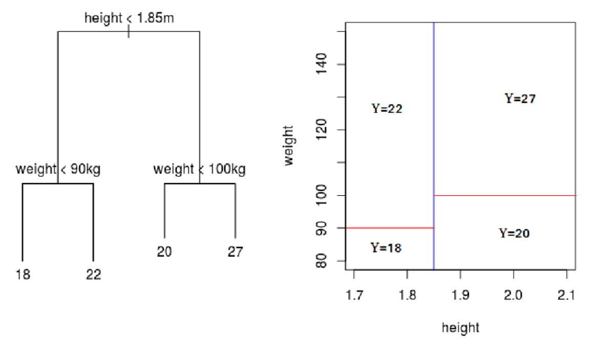
The idea of regression trees is to approximate $f_{h}(\boldsymbol{X}_{t})$ by

h_{D}(\boldsymbol{X}_{t})=\sum_{j=1}^{J_{T}}\beta_{j}I_{j}(\boldsymbol{X}_{t}),\quad\textnormal{where}\quad I_{k}(\boldsymbol{X}_{t})=\begin{cases}1&\textnormal{if }\boldsymbol{X}_{t}\in\mathcal{R}_{j},\\ 0&\textnormal{otherwise}.\end{cases}

From the above expression, it becomes clear that the approximation of $f_{h}(\cdot)$ is equivalent to a linear regression on $J_{T}$ dummy variables, where $I_{j}(\boldsymbol{X}_{t})$ is a product of indicator functions.

Let $J:=J_{T}$ and $N:=N_{T}$ be, respectively, the number of terminal nodes (regions, leaves) and parent nodes. Different regions are denoted as $\mathcal{R}_{1},\ldots,\mathcal{R}_{J}$ . The root node at position $0$ . The parent node at position $j$ has two split (child) nodes at positions $2j+1$ and $2j+2$ . Each parent node has a threshold (split) variable associated, $X_{s_{j}t}$ , where $s_{j}\in\mathbb{S}=\{1,2,\ldots,p\}$ . Define $\mathbb{J}$ and $\mathbb{T}$ as the sets of parent and terminal nodes, respectively. Figure 6 gives an example. In the example, the parent nodes are $\mathbb{J}=\{0,2,5\}$ and the terminal nodes are $\mathbb{T}=\{1,6,11,12\}$ .

\Tree[.{Parent\\ node0}{Terminal\\ node1\\ (Region1)}[.{Parent\\ node2}[.{Parent\\ node5}{Terminal\\ node11\\ (Region2)}{Terminal\\ node12\\ (Region3)}]{Terminal\\ node6\\ (Region4)}]]

Figure 6: Example of tree with labels.

Therefore, we can write the approximating model as

h_{D}(\boldsymbol{X}_{t})=\sum_{i\in\mathbb{T}}\beta_{i}B_{\mathbb{J}i}\left(\boldsymbol{X}_{t};\boldsymbol{\theta}_{i}\right),

(3.6)

where

B_{\mathbb{J}i}\left(\boldsymbol{X}_{t};\boldsymbol{\theta}_{i}\right)=\prod_{j\in\mathbb{J}}I(X_{s_{j},t};c_{j})^{\frac{n_{i,j}(1+n_{i,j})}{2}}\times\left[1-I(X_{s_{j},t};c_{j})\right]^{(1-n_{i,j})(1+n_{i,j})},

(3.7)

I(X_{s_{j},t};c_{j})=\begin{cases}1&\textnormal{if}\,X_{s_{j},t}\leq c_{j}\\ 0&\textnormal{otherwise},\end{cases}

n_{i,j}=\begin{cases}-1&\text{if the path to leaf }\,i\,\text{does not include parent node }j;\\ 0&\text{if the path to leaf }\,i\,\text{include the {right-hand} child of parent node }j;\\ 1&\text{if the path to leaf }\,i\,\text{include the {left-hand} child of parent node }j.\\ \end{cases}

$\mathbb{J}_{i}$ : indexes of parent nodes included in the path to leaf $i$ . $\boldsymbol{\theta}_{i}=\{c_{k}\}$ such that $k\in\mathbb{J}_{i}$ , $i\in\mathbb{T}$ and $\sum_{j\in\mathbb{J}}B_{\mathbb{J}i}\left(\boldsymbol{X}_{t};\boldsymbol{\theta}_{j}\right)=1$ .

3.2.1 Random Forests

Random Forest (RF) is a collection of regression trees, each specified in a bootstrap sample of the original data. The method was originally proposed by Breiman 2001. Since we are dealing with time series, we use a block bootstrap. Suppose there are $B$ bootstrap samples. For each sample $b$ , $b=1,\ldots,B$ , a tree with $K_{b}$ regions is estimated for a randomly selected subset of the original regressors. $K_{b}$ is determined in order to leave a minimum number of observations in each region. The final forecast is the average of the forecasts of each tree applied to the original data:

\widehat{Y}_{t+h|t}=\frac{1}{B}\sum_{b=1}^{B}\left[\sum_{i=1}^{\mathbb{T}_{b}}\widehat{\beta}_{i,b}B_{\mathbb{J}i,b}(\boldsymbol{X}_{t};\widehat{\boldsymbol{\theta}}_{i,b})\right].

The theory for RF models has been developed only to independent and identically distributed random variables. For instance, Scornet et al. 2015 proves consistency of the RF approximation to the unknown function $f_{h}(\boldsymbol{X}_{t})$ . More recently, Wager and Athey 2018 proved consistency and asymptotic normality of the RF estimator.

3.2.2 Boosting Regression Trees

Boosting is another greedy method to approximate nonlinear functions that uses base learners for a sequential approximation. The model we consider here, called Gradient Boosting, was introduced by Friedman 2001 and can be seen as a Gradient Descendent method in functional space.

The study of statistical properties of the Gradient Boosting is well developed for independent data. For example, for regression problems, Duffy and Helmbold 2002 derived bounds on the convergence of boosting algorithms using assumptions on the performance of the base learner. Zhang and Yu 2005 proves convergence, consistency and results on the speed of convergence with mild assumptions on the base learners. Bühlmann 2002 shows similar results for consistency in the case of $\ell_{2}$ loss functions and three base models. Since boosting indefinitely leads to overfitting problems, some authors have demonstrated the consistency of boosting with different types of stopping rules, which are usually related to small step sizes, as suggested by Friedman 2001. Some of these works include boosting in classification problems and gradient boosting for both classification and regression problems. See, for instance, Jiang 2004; Lugosi and Vayatis 2004; Bartlett and M. Traskin 2007; Zhang and Yu 2005; Bühlmann 2006; Bühlmann 2002.

Boosting is an iterative algorithm. The idea of boosted trees is to, at each iteration, sequentially refit the gradient of the loss function by small trees. In the case of quadratic loss as considered in this paper, the algorithm simply refit the residuals from the previous iteration.

Algorithm (2) presents the simplified boosting procedure for a quadratic loss. It is recommended to use a shrinkage parameter $v\in(0,1]$ to control the learning rate of the algorithm. If $v$ is close to 1, we have a faster convergence rate and a better in-sample fit. However, we are more likely to have over-fitting and produce poor out-of-sample results. Additionally, the derivative is highly affected by over-fitting, even if we look at in-sample estimates. A learning rate between 0.1 and 0.2 is recommended to maintain a reasonable convergence ratio and to limit over-fitting problems.

Algorithm 2.

The boosting algorithm is defined as the following steps.

1.

Initialize $\phi_{i0}=\bar{Y}:=\frac{1}{T}\sum_{t=1}^{T}Y_{t}$ ;
2.
For $m=1,\dots,M$ :
1. (a)
  
  Make $U_{tm}=Y_{t}-\phi_{tm-1}$
2. (b)
  
  Grow a (small) Tree model to fit $u_{tm}$ , $\widehat{u}_{tm}=\sum_{i\in\mathbb{T}_{m}}\widehat{\beta}_{im}B_{\mathbb{J}_{m}i}(\boldsymbol{X}_{t};\widehat{\boldsymbol{\theta}}_{im})$
3. (c)
  
  Make $\rho_{m}=\arg\underset{\rho}{\min}\sum_{t=1}^{T}[u_{tm}-\rho\widehat{u}_{tm}]^{2}$
4. (d)
  
  Update $\phi_{tm}=\phi_{tm-1}+v\rho_{m}\widehat{u}_{tm}$

The final fitted value may be written as

\begin{split}\widehat{Y}_{t+h}&=\bar{Y}+\sum_{m=1}^{M}v\rho_{m}\widehat{u}_{tm}\\ &=\bar{Y}+\sum_{m=1}^{M}v\widehat{\rho}_{m}\sum_{k\in\mathbb{T}_{m}}\widehat{\beta}_{km}B_{\mathbb{J}_{m}k}(\boldsymbol{X}_{t};\widehat{\boldsymbol{\theta}}_{km})\end{split}

(3.8)

3.3 Inference

Conducting inference in nonlinear ML methods is tricky. One possible way is to follow Medeiros et al. 2006, Medeiros and Veiga 2005 and Suarez-Fariñas et al. 2004 and interpret particular nonlinear ML specifications as parametric models, as for example, general forms of smooth transition regressions. However, this approach restricts the application of ML methods to very specific settings. An alternative, is to consider models that can be cast in the sieves framework as described earlier. This is the case of splines and feed-forward NNs, for example. In this setup, Chen and Shen 1998 and Chen 2007 derived, under regularity conditions, the consistency and asymptotically normality of the estimates of a semi-parametric sieve approximations. Their setup is defined as follows:

Y_{t+h}=\boldsymbol{\beta}_{0}^{\prime}\boldsymbol{X}_{t}+f(\boldsymbol{X}_{t})+U_{t+h},

where $f(\boldsymbol{X}_{t})$ is a nonlinear function that is nonparametrically modeled by sieve approximations. Chen and Shen 1998 and Chen 2007 consider both the estimation of the linear and nonlinear components of the model. However, their results are derived under the case where the dimension of $\boldsymbol{X}_{t}$ is fixed.

Recently, Chernozhukov et al. 2017 and Chernozhukov et al. 2018 consider the case where the number of covariates diverge as the sample size increases in a very general setup. In this case the asymptotic results in Chen and Shen 1998 and Chen 2007 are not valid and the authors put forward the so-called double ML methods as a nice generalization to the results of Belloni et al. 2014. For Deep Neural Networks, Farrell et al. 2021 consider semiparametric inference and establish nonasymptotic high probability bounds. Consequently, the authors are able to derive rates of convergence that are sufficiently fast to allow them to establish valid second‐step inference after first‐step estimation with deep learning. Nevertheless, the above papers do not include the case of time-series models.

More specifically to the case of Random Forests, asymptotic and inferential results are derived in Scornet et al. 2015 and Wager and Athey 2018 for the case of IID data. More recently, Davis and Nielsen 2020 prove a uniform concentration inequality for regression trees built on nonlinear autoregressive stochastic processes and prove consistency for a large class of random forests. Finally, it is worth mentioning the interesting work of Borup et al. 2020. In their paper, the authors show that proper predictor targeting controls the probability of placing splits along strong predictors and improves prediction.

4 Other Methods

4.1 Bagging

The term bagging means Bootstrap Aggregating and was proposed by Breiman 1996 to reduce the variance of unstable predictors⁸⁸ 8 An unstable predictor has large variance. Intuitively, small changes in the data yield large changes in the predictive model. It was popularized in the time series literature by Inoue and Kilian 2008, who to construct forecasts from multiple regression models with local-to-zero regression parameters and errors subject to possible serial correlation or conditional heteroscedasticity. Bagging is designed for situations in which the number of predictors is moderately large relative to the sample size.

The bagging algorithm in time series settings have to take into account the time dependence dimension when constructing the bootstrap samples.

Algorithm 3 (Bagging for Time-Series Models).

The Bagging algorithm is defined as follows.

1.

Arrange the set of tuples $\left(y_{t+h},\boldsymbol{x}^{\prime}_{t}\right)$ , $t=h+1,\ldots,T$ , in the form of a matrix $\boldsymbol{V}$ of dimension $(T-h)\times n$ .
2.

Construct (block) bootstrap samples of the form $\left\{\left(y_{(i)2}^{\ast},\boldsymbol{x}^{\prime*}_{(i)2}\right),\ldots,\left(y^{*}_{(i)T},\boldsymbol{x}^{\prime*}_{(i)T}\right)\right\}$ , $i=1,\ldots,B$ , by drawing blocks of $M$ rows of $\boldsymbol{V}$ with replacement.

Compute the $i$ th bootstrap forecast as

\widehat{y}^{\ast}_{(i)t+h|t}=\begin{cases}0&\text{if }|t^{*}_{j}|<c\,\forall j,\\ \widehat{\boldsymbol{\lambda}}_{(i)}^{*}\widetilde{\boldsymbol{x}}^{*}_{(i)t}&\text{otherwise},\end{cases}

(4.1)

where $\widetilde{\boldsymbol{x}}^{*}_{(i)t}:=\boldsymbol{S}_{(i)t}^{*}\boldsymbol{z}_{(i)t}^{*}$ and $\boldsymbol{S}_{t}$ is a diagonal selection matrix with $j$ th diagonal element given by

\mathbb{I}_{\{|t_{j}|>c\}}=\begin{cases}1&\text{if }|t_{j}|>c,\\ 0&\text{otherwise,}\end{cases}

$c$ is a pre-specified critical value of the test. $\widehat{\boldsymbol{\lambda}}_{(i)}^{*}$ is the OLS estimator at each bootstrap repetition.

4.

Compute the average forecasts over the bootstrap samples:

$\tilde{y}_{t+h|t}=\frac{1}{B}\sum_{i=1}^{B}\widehat{y}^{\ast}_{(i)t|t-1}.$

In algorithm 3, above, one requires that it is possible to estimate and conduct inference in the linear model. This is certainly infeasible if the number of predictors is larger than the sample size ( $n>T$ ), which requires the algorithm to be modified. Garcia et al. 2017 and Medeiros et al. 2021 adopt the following changes of the algorithm:

Algorithm 4 (Bagging for Time-Series Models and Many Regressors).

The Bagging algorithm is defined as follows.

0.

Run $n$ univariate regressions of $y_{t+h}$ on each covariate in $\boldsymbol{x}_{t}$ . Compute $t$ -statistics and keep only the ones that turn out to be significant at a given pre-specified level. Call this new set of regressors as $\check{\boldsymbol{x}}_{t}$
1–4.

Same as before but with $\boldsymbol{x}_{t}$ replaced by $\check{\boldsymbol{x}}_{t}$ .

4.2 Complete Subset Regression

Complete Subset Regression (CSR) is a method for combining forecasts developed by Elliott et al. 2013; Elliott et al. 2015. The motivation was that selecting the optimal subset of $\boldsymbol{X}_{t}$ to predict $Y_{t+h}$ by testing all possible combinations of regressors is computationally very demanding and, in most cases, unfeasible. For a given set of potential predictor variables, the idea is to combine forecasts by averaging⁹⁹ 9 It is possible to combine forecasts using any weighting scheme. However, it is difficult to beat uniform weighting Genre et al. 2013. all possible linear regression models with fixed number of predictors. For example, with $n$ possible predictors, there are $n$ unique univariate models and

n_{k,n}=\frac{n!}{(n-k)!k!}

different $k$ -variate models for $k\leq K$ . The set of models for a fixed value of $k$ as is known as the complete subset.

When the set of regressors is large the number of models to be estimated increases rapidly. Moreover, it is likely that many potential predictors are irrelevant. In these cases it was suggested that one should include only a small, $k$ , fixed set of predictors, such as five or ten. Nevertheless, the number of models still very large, for example, with $n=30$ and $k=8$ , there are $5,852,925$ regression. An alternative solution is to follow Garcia et al. 2017 and Medeiros et al. 2021 and adopt a similar strategy as in the case of Bagging high-dimensional models. The idea is to start fitting a regression of $Y_{t+h}$ on each of the candidate variables and save the $t$ -statistics of each variable. The $t$ -statistics are ranked by absolute value, and we select the $\tilde{n}$ variables that are more relevant in the ranking. The CSR forecast is calculated on these variables for different values of $k$ . This approach is based on the the Sure Independence Screening of Fan and Lv 2008, extended to dependent by Yousuf 2018, that aims to select a superset of relevant predictors among a very large set.

4.3 Hybrid Methods

Recently, Medeiros and Mendes 2013 proposed the combination of LASSO-based estimation and NN models. The idea is to construct a feedforward single-hidden layer NN where the parameters of the nonlinear terms (neurons) are randomly generated and the linear parameters are estimated by LASSO (or one of its generalizations). Similar ideas were also considered by Kock and Teräsvirta 2014 and Kock and Teräsvirta 2015.

Trapletti et al. 2000 and Medeiros et al. 2006 proposed to augment a feedforward shallow NN by a linear term. The motivation is that the nonlinear component should capture only the nonlinear dependence, making the model more interpretable. This is in the same spirit of the semi-parametric models considered in Chen 2007.

Inspired by the above ideas, Medeiros et al. 2021 proposed combining random forests with adaLASSO and OLS. The authors considered two specifications. In the first one, called RF/OLS, the idea is to use the variables selected by a Random Forest in a OLS regression. The second approach, named adaLASSO/RF, works in the opposite direction. First select the variables by adaLASSO and than use them in a Random Forest model. The goal is to disentangle the relative importance of variable selection and nonlinearity to forecast inflation.

Recently, Diebold and Shin 2019 propose the “partially-egalitarian” LASSO to combine survey forecasts. More specifically, the procedure sets some combining weights to zero and shrinks the survivors toward equality. Therefore, the final forecast will be close related to the simple average combination of the survived forecasts. Although the paper considers survey forecasts, the method is quite general and can be applied to any set of forecasts. As pointed out by the authors, optimally-regularized regression-based combinations and subset-average combinations are very closely connected. Diebold et al. 2021 extended the ideas in Diebold and Shin 2019 in order to construct regularized mixtures of density forecasts. Both papers shed light on how machine learning methods can be used to optimally combine a large set of forecasts.

5 Forecast Comparison

With the advances in the ML literature, the number of available forecasting models and methods have been increasing at a fast pace. Consequently, it is very important to apply statistical tools to compare different models. The forecasting literature provides a number of tests since the seminal paper by Diebold and Mariano 1995 that can be applied as well to the ML models described in this survey.

In the Diebold and Mariano’s (1995) test, two competing methods have the same unconditional expected loss under the null hypothesis, and the test can be carried out using a simple t-test. A small sample adjustment was developed by Harvey et al. 1997. See also the recent discussion in Diebold 2015. One drawback of the Diebold and Mariano’s (1995) test is that its statistic diverges under null when the competing models are nested. However, Giacomini and White 2006 show that the test is valid if the forecasts are derived from models estimated in a rolling window framework. Recently, McCracken 2020 shows that if the estimation window is fixed, the Diebold and Mariano’s (1995) statistic may diverge under the null. Therefore, it is very important that the forecasts are computed in a rolling window scheme.

In order to accommodate cases where there are more than two competing models, an unconditional superior predictive ability (USPA) test was proposed by White 2000. The null hypothesis states that a benchmark method outperforms a set of competing alternatives. However, Hansen 2005 showed that White’s (2000) test can be very conservative when there are competing methods that are inferior to the benchmark. Another important contribution to the forecasting literature is the model confidence set (MCS) proposed by Hansen et al. 2011. A MCS is a set of competing models that is built in a way to contain the best model with respect to a certain loss function and with a given level of confidence. The MCS acknowledges the potential limitations of the dataset, such that uninformative data yield a MCS with a large number models, whereas informative data yield a MCS with only a few models. Importantly, the MCS procedure does not assume that a particular model is the true one.

Another extension of the Diebold and Mariano’s (1995) test is the conditional equal predictive ability (CEPA) test proposed by Giacomini and White 2006. In practical applications, it is important to know not only if a given model is superior but also when it is better than the alternatives. Recently, Li et al. 2020 proposed a very general framework to conduct conditional predictive ability tests.

In summary, it is very important to compare the forecasts from different ML methods and the literature provides a number of tests that can be used.

6 Applications of Machine Learning Methods to Economic and Financial Forecasting

6.1 Linear Methods

Penalized regressions are now an important option in the toolkit of applied economists are there is a vast literature considering the use of such techniques to economics and financial forecasting.

Macroeconomic forecasting is certainly one of the most successful applications of penalized regressions. Medeiros and Mendes 2016 applied the adaLASSO to forecasting US inflation and showed that the method outperforms the linear autoregressive and factor models. Medeiros and Vasconcelos 2016 show that high-dimensional linear models produce, on average, smaller forecasting errors for macroeconomic variables when a large set of predictors is considered. Their results also indicate that a good selection of the adaLASSO hyperparameters reduces forecasting errors. Garcia et al. 2017 show that high-dimensional econometric models, such as shrinkage and complete subset regression, perform very well in real time forecasting of Brazilian inflation in data-rich environments. The authors combine forecasts of different alternatives and show that model combination can achieve superior predictive performance. Smeeks and Wijler 2018 consider an application to a large macroeconomic US dataset and demonstrate that penalized regressions are very competitive. Medeiros et al. 2021 conduct a vast comparison of models to forecast US inflation and showed the penalized regressions were far superior than several benchmarks, including factor models. Ardia et al. 2019 introduce a general text sentiment framework that optimizes the design for forecasting purposes and apply it to forecasting economic growth in the US. The method includes the use of the elastic net for sparse data-driven selection and the weighting of thousands of sentiment values. Tarassow 2019 consider penalized VARs to forecast six different economic uncertainty variables for the growth of the real M2 and real M4 Divisia money series for the US using monthly data. Uematsu and Tanaka 2019 consider high-dimensional forecasting and variable selection via folded-concave penalized regressions. The authors forecast quarterly US gross domestic product data using a high-dimensional monthly data set and the mixed data sampling (MIDAS) framework with penalization. See also Babii et al. 2020c and Babii et al. 2020b.

There is also a vast list of applications in empirical finance. Elliott et al. 2013 find that combinations of subset regressions can produce more accurate forecasts of the equity premium than conventional approaches based on equal-weighted forecasts and other regularization techniques. Audrino and Knaus 2016 used LASSO-based methods to estimated forecasting models for realized volatilities. Callot et al. 2017 consider modelling and forecasting large realized covariance matrices of the 30 Dow Jones stocks by penalized vector autoregressive (VAR) models. The authors find that penalized VARs outperform the benchmarks by a wide margin and improve the portfolio construction of a mean-variance investor. Chinco et al. 2019 use the LASSO to make 1-minute-ahead return forecasts for a vast set of stocks traded at the New York Stock Exchange. The authors provide evidence that penalized regression estimated by the LASSO boost out-of-sample predictive power by choosing predictors that trace out the consequences of unexpected news announcements.

6.2 Nonlinear Methods

There are many papers on the application of nonlinear ML methods to economic and financial forecasting. Most of the papers focus on NN methods, specially the ones from the early literature.

With respect to the early papers, most of the models considered were nonlinear versions of autoregressive models. At best, a small number of extra covariates were included. See, for example, Teräsvirta et al. 2005 and the references therein. In the majority of the papers, including Teräsvirta et al. 2005, there was no strong evidence of the superiority of nonlinear models as the differences in performance were marginal. Other examples from the early literature are Swanson and White 1995, Swanson and White 1997a, Swanson and White 1997b, Balkin and Ord 2000, Tkacz 2001, Medeiros et al. 2001, and Heravi et al. 2004.

More recently, with the availability of large datasets, nonlinear models are back to the scene. For example, Medeiros et al. 2021 show that, despite the skepticism of the previous literature on inflation forecasting, ML models with a large number of covariates are systematically more accurate than the benchmarks for several forecasting horizons and show that Random Forests dominated all other models. The good performance of the Random Forest is due not only to its specific method of variable selection but also the potential nonlinearities between past key macroeconomic variables and inflation. Other successful example is Gu et al. 2020. The authors show large economic gains to investors using ML forecasts of future stock returns based on a very large set of predictors. The best performing models are tree-based and neural networks. Coulombe et al. 2020 show significant gains when nonlinear ML methods are used to forecast macroeconomic time series. Borup and Schütte 2020 consider penalized regressions, ensemble methods, and random forest to forecast employment growth in the United States over the period 2004–2019 using Google search activity. Their results strongly indicate that Google search data have predictive power. Borup et al. 2020 compute now- and backcasts of weekly unemployment insurance initial claims in the US based on a rich set of daily Google Trends search-volume data and machine learning methods.

6.3 Empirical Illustration

In this section we illustrate the use of some of the methods reviewed in this paper to forecast daily realized variance of the Brazilian Stock Market index (BOVESPA). We use as regressors information from other major indexes, namely, the S&P500 (US), the FTSE100 (United Kingdom), DAX (Germany), Hang Seng (Hong Kong), and Nikkei (Japan). Our measure of realized volatility is constructed by aggregating intraday returns sample at the 5-minute frequency. The data were obtained from the Oxford-Man Realized Library at Oxford University.¹⁰¹⁰ 10 https://realized.oxford-man.ox.ac.uk/data/assets

For each stock index, we define the realized variance as

RV_{t}=\sum_{s=1}^{S}r^{2}_{st},

where $r_{st}$ is the log return sampled at the five-minute frequency. $S$ is the number of available returns at day $t$ .

The benchmark model is the Heterogeneous Autoregressive (HAR) model proposed by Corsi 2009:

\log RV_{t+1}=\beta_{0}+\beta_{1}\log RV_{t}+\beta_{5}\log RV_{5,t}+\beta_{2}2\log RV_{22,t}+U_{t+1},

(6.1)

where $RV_{t}$ is daily realized variance of the BOVESPA index,

\begin{split}RV_{5,t}&=\frac{1}{5}\sum_{i=0}^{4}RV_{t-i},\quad\textnormal{and}\\ RV_{22,t}&=\frac{1}{22}\sum_{i=0}^{21}RV_{t-i}.\end{split}

As alternatives we consider a extended HAR model with additional regressors estimated by adaLASSO. We include as extra regressors the daily past volatility of the other five indexes considered here. The model has a total of eight candidate predictors. Furthermore, we consider two nonlinear alternatives using all predictors: a random forest and shallow and deep neural networks.

The realized variances of the different indexes are illustrated in Figure 7. The data starts in February 2, 2000 and ends in May 21, 2020, a total of 4,200 observations. The sample includes two periods of very high volatility, namely the financial crisis of 2007-2008 and the Covid-19 pandemics of 2020. We consider a rolling window exercise, were we set 1,500 observations in each window. The models are re-estimated every day.

Several other authors have estimated nonlinear and machine learning models to forecast realized variances. McAleer and Medeiros 2008 considered a smooth transition version of the HAR while Hillebrand and Medeiros 2016 considered the combination of smooth transitions, long memory and neural network models. Hillebrand and Medeiros 2010 and McAleer and Medeiros 2011 combined NN models with bagging and Scharth and Medeiros 2009 considered smooth transition regression trees. The use of LASSO and its generalizations to estimate extensions of the HAR model was proposed by Audrino and Knaus 2016.

Although the models are estimated in logarithms, we report the results in levels, which in the end is the quantity of interest. We compare the models according to the Mean Squared Error (MSE) and the QLIKE metric.

The results are shown in Table 1. The table reports for each model, the mean squared error (MSE) and the QLIKE statistics as a ratio to the HAR benchmark. Values smaller than one indicates that the model outperforms the HAR. The asterisks indicate the results of the Diebold-Mariano test of equal forecasting performance. *,**, and ***, indicate rejection of the null of equal forecasting ability at the 10%, 5% and 1%, respectively. We report results for the full out-of-sample period, the financial crisis years (2007-2008) and the for 2020 as a way to capture the effects of the Covid-19 pandemics on the forecasting performance of different models.

As we can see from the tables the ML methods considered here outperform the HAR benchmark. The winner model is definitely the HAR model with additional regressors and estimated with adaLASSO. The performance improves during the high volatility periods and the gains reach 10% during the Covid-19 pandemics. Random Forests do not perform well. On the other hand NN models with different number of hidden layers outperform the benchmark.

Figure 7: Realized variance of different stock indexes

Table 1: Forecasting Results

The table reports for each model, the mean squared error (MSE) and the QLIKE statistics as a ratio to the HAR benchmark. Values smaller than one indicates that the model outperforms the HAR. The asterisks indicate the results of the Diebold-Mariano test of equal forecasting performance. *,**, and ***, indicate rejection of the null of equal forecasting ability at the 10%, 5% and 1%, respectively.

Model	MSE	QLIKE	MSE	QLIKE	MSE	QLIKE
	Full Sample		2007-2008		2020
HARX-LASSO	$0.96^{**}$	$0.98$	$0.98^{*}$	$0.96$	$0.90^{***}$	$0.90$
Random Forest	$1.00$	$1.02$	$0.95^{***}$	$0.98$	$1.13^{**}$	$1.03^{*}$
Neural Network (1)	$0.99^{**}$	$0.99$	$0.97^{**}$	$0.98$	$0.99$	$0.99$
Neural Network (3)	$0.99^{**}$	$0.99$	$0.98^{*}$	$0.99$	$0.99$	$0.99$
Neural Network (5)	$0.90^{**}$	$0.99$	$0.98^{*}$	$0.99$	$0.99$	$0.99$

7 Conclusions and the Road Ahead

In this paper we present a non-exhaustive review of the most of the recent developments in machine learning and high-dimensional statistics to time-series modeling and forecasting. We presented both linear and nonlinear alternatives. Furthermore, we consider ensemble and hybrid models. Finally, we briefly discuss tests for superior predictive ability.

Among linear specification, we pay special attention to penalized regression (Ridge, LASSO and its generalizations, for example) and ensemble methods (Bagging and Complete Subset Regression). Although, there has been major theoretical advances in the literature on penalized linear regression models for dependent data, the same is not true for ensemble methods. The theoretical results for Bagging are so far based on independent data and the results for complete subset regression are quite limited.

With respect to nonlinear ML methods, we focused on neural networks and tree-based methods. Theoretical results for random forests and boosted trees have been developed only to independent and identically distributed data and in the case of a low dimensional set of regressors. For shallow neural networks, Chen et al. 2007 and Chen 2007 provide some theoretical results for dependent data in the low dimensional case. The behavior of such models in high-dimensions is still under study. The same is true for deep neural networks.

Nevertheless, the recent empirical evidence shows that nonlinear machine learning models combined with large datasets can be extremely useful for economic forecasting.

As a direction for further developments we list the following points:

1.

Develop results for Bagging and Boosting for dependent data.
2.

Show consistency and asymptotic normality of the random forecast estimator of the unknown function $f_{h}(\boldsymbol{X}_{t})$ when the data are dependent.
3.

Derive a better understanding of the variable selection mechanism of nonlinear ML methods.
4.

Develop inferential methods to access variable importance in nonlinear ML methods.
5.

Develop models based on unstructured data, such as text data, to economic forecasting.
6.

Evaluate ML models for nowcasting.
7.

Evaluate ML in very unstable environments with many structural breaks.

Finally, we would like to point that we left a number of other interesting ML methods out of this survey, such as, for example, Support Vector Regressions, autoenconders, nonlinear factor models, and many more. However, we hope that the material presented here can be of value to anyone interested of applying ML techniques to economic and/or financial forecasting.

References

Adámek et al. (2020) Adámek, R., S. Smeekes, and I. Wilms (2020). LASSO inference for high-dimensional time series. Technical Report 2007.10952, arxiv.
Ardia et al. (2019) Ardia, D., K. Bluteau, and K. Boudt (2019). Questioning the news about economic growth: Sparse forecasting using thousands of news-based sentiment values. International Journal of Forecasting 35, 1370–1386.
Audrino and Knaus (2016) Audrino, F. and S. D. Knaus (2016). Lassoing the HAR model: A model selection perspective on realized volatility dynamics. Econometric Reviews 35, 1485–1521.
Babii et al. (2020a) Babii, A., E. Ghysels, and J. Striaukas (2020a). Inference for high-dimensional regressions with heteroskedasticity and autocorrelation. Technical Report 1912.06307, arxiv.
Babii et al. (2020b) Babii, A., E. Ghysels, and J. Striaukas (2020b). Machine learning panel data regressions with an application to nowcasting price earnings ratios. Technical Report 2008.03600, arxiv.
Babii et al. (2020c) Babii, A., E. Ghysels, and J. Striaukas (2020c). Machine learning time series regressions with an application to nowcasting. Technical Report 2005.14057, arxiv.
Balkin and Ord (2000) Balkin, S. D. and J. K. Ord (2000). Automatic neural network modeling for univariate time series. International Journal of Forecasting 16, 509–515.
Barron (1993) Barron, A. (1993). Universal approximation bounds for superpositions of a sigmoidal function. IEEE Transactions on Information Theory 39, 930–945.
Bartlett and M. Traskin (2007) Bartlett, P. and M. M. Traskin (2007). AdaBoost is consistent. Journal of Machine Learning Research 8, 2347–2368.
Basu and Michailidis (2015) Basu, S. and G. Michailidis (2015). Regularized estimation in sparse high-dimensional time series models. Annals of Statistics 43, 1535–1567.
Belloni et al. (2014) Belloni, A., V. Chernozhukov, and C. Hansen (2014). Inference on treatment effects after selection amongst high-dimensional controls. Review of Economic Studies 81, 608–650.
Bühlmann (2006) Bühlmann, P. (2006). Boosting for high-dimensional linear models. Annals of Statistics 34, 559–583.
Borup et al. (2020) Borup, D., B. Christensen, N. Mühlbach, and M. Nielsen (2020). Targeting predictors in random forest regression. Technical Report 2004.01411, arxiv.
Borup et al. (2020) Borup, D., D. Rapach, and E. Schütte (2020). Now- and backcasting initial claims with high-dimensional daily internet search-volume data. Technical Report 3690832, SSRN.
Borup and Schütte (2020) Borup, D. and E. Schütte (2020). In search of a job: Forecasting employment growth using Google trends. Journal of Business and Economic Statistics. forthcoming.
Breiman (1996) Breiman, L. (1996). Bagging predictors. Machine Learning 24, 123–140.
Breiman (2001) Breiman, L. (2001). Random forests. Machine Learning 45, 5–32.
Bühlmann (2002) Bühlmann, P. L. (2002). Consistency for l2boosting and matching pursuit with trees and tree-type basis functions. In Research report/Seminar für Statistik, Eidgenössische Technische Hochschule (ETH), Volume 109. Seminar für Statistik, Eidgenössische Technische Hochschule (ETH).
Callot et al. (2013) Callot, L., A.B., and Kock (2013). Oracle efficient estimation and forecasting with the adaptive LASSO and the adaptive group LASSO in vector autoregressions. In N. Haldrup, M. Meitz, and P. Saikkonen (Eds.), Essays in Nonlinear Time Series Econometrics. Oxford University Press.
Callot et al. (2017) Callot, L., A. Kock, and M. Medeiros (2017). Modeling and forecasting large realized covariance matrices and portfolio choice. Journal of Applied Econometrics 32, 140–158.
Chan and Chen (2011) Chan, K.-S. and K. Chen (2011). Subset ARMA selection via the adaptive LASSO. Statistics and its Interface 4, 197–205.
Chen et al. (2001) Chen, S., D. Donoho, and M. Saunders (2001). Atomic decomposition by basis pursuit. SIAM review 43, 129–159.
Chen (2007) Chen, X. (2007). Large sample sieve estimation of semi-nonparametric models. In J. Heckman and E. Leamer (Eds.), Handbook of Econometrics. Elsevier.
Chen et al. (2007) Chen, X., J. Racine, and N. Swanson (2007). Semiparametric ARX neural-network models with an application to forecasting inflation. IEEE Transactions on Neural Networks 12, 674–683.
Chen and Shen (1998) Chen, X. and S. Shen (1998). Sieve extremum estimates for weakly dependent data. Econometrica 66, 289–314.
Chernozhukov et al. (2017) Chernozhukov, V., D. Chetverikov, M. Demirer, E. Duflo, C. Hansen, and W. Newey (2017). Double/debiased/neyman machine learning of treatment effects. American Economic Review 107, 261–265.
Chernozhukov et al. (2018) Chernozhukov, V., D. Chetverikov, M. Demirer, E. Duflo, C. Hansen, W. Newey, and J. Robins (2018). Double/debiased machine learning for treatment and structural parameters. Econometrics Journal 21, C1–C68.
Chinco et al. (2019) Chinco, A., A. Clark-Joseph, and M. Ye (2019). Sparse signals in the cross-section of returns. Journal of Finance 74, 449–492.
Corsi (2009) Corsi, F. (2009). A simple long memory model of realized volatility. Journal of Financial Econometrics 7, 174–196.
Coulombe et al. (2020) Coulombe, P., M. Leroux, D. Stevanovic, and S. Surprenant (2020). How is machine learning useful for macroeconomic forecasting? Technical report, University of Pennsylvania.
Cybenko (1989) Cybenko, G. (1989). Approximation by superposition of sigmoidal functions. Mathematics of Control, Signals, and Systems 2, 303–314.
Davis and Nielsen (2020) Davis, R. and M. Nielsen (2020). Modeling of time series using random forests: Theoretical developments. Electronic Journal of Statistics 14, 3644–3671.
Diebold (2015) Diebold, F. (2015). Comparing predictive accuracy, twenty years later: A personal perspective on the use and abuse of Diebold-Mariano tests. Journal of Business and Economic Statistics 33, 1–9.
Diebold and Shin (2019) Diebold, F. and M. Shin (2019). Machine learning for regularized survey forecast combination: Partially-egalitarian LASSO and its derivatives. International Journal of Forecasting 35, 1679–1691.
Diebold et al. (2021) Diebold, F., M. Shin, and B. Zhang (2021). On the aggregation of probability assessments: Regularized mixtures of predictive densities for Eurozone inflation and real interest rates. Technical Report 2012.11649, arxiv.
Diebold and Mariano (1995) Diebold, F. X. and R. S. Mariano (1995). Comparing predictive accuracy. Journal of Business and Economic Statistics 13, 253–263.
Duffy and Helmbold (2002) Duffy, N. and D. Helmbold (2002). Boosting methods for regression. Machine Learning 47, 153–200.
Elliott et al. (2013) Elliott, G., A. Gargano, and A. Timmermann (2013). Complete subset regressions. Journal of Econometrics 177(2), 357–373.
Elliott et al. (2015) Elliott, G., A. Gargano, and A. Timmermann (2015). Complete subset regressions with large-dimensional sets of predictors. Journal of Economic Dynamics and Control 54, 86–110.
Elliott and Timmermann (2008) Elliott, G. and A. Timmermann (2008). Economic forecasting. Journal of Economic Literature 46, 3–56.
Elliott and Timmermann (2016) Elliott, G. and A. Timmermann (2016). Forecasting in economics and finance. Annual Review of Economics 8, 81–110.
Fan and Li (2001) Fan, J. and R. Li (2001). Variable selection via nonconcave penalized likelihood and its oracle properties. Journal of the American Statistical Association 96, 1348–1360.
Fan and Lv (2008) Fan, J. and J. Lv (2008). Sure independence screening for ultrahigh dimensional feature space. Journal of the Royal Statistical Society, Series B 70, 849–911.
Fan et al. (2014) Fan, J., L. Xue, and H. Zou (2014). Strong oracle optimality of folded concave penalized estimation. Annals of Statistics 42, 819–849.
Farrell et al. (2021) Farrell, M., T. Liang, and S. Misra (2021). Deep neural networks for estimation and inference. Econometrica 89, 181–213.
Foresee and Hagan (1997) Foresee, F. D. and M. . T. Hagan (1997). Gauss-newton approximation to Bayesian regularization. In IEEE International Conference on Neural Networks (Vol. 3), New York, pp. 1930–1935. IEEE.
Friedman (2001) Friedman, J. (2001). Greedy function approximation: a gradient boosting machine. Annals of Statistics 29, 1189–1232.
Funahashi (1989) Funahashi, K. (1989). On the approximate realization of continuous mappings by neural networks. Neural Networks 2, 183–192.
Garcia et al. (2017) Garcia, M., M. Medeiros, and G. Vasconcelos (2017). Real-time inflation forecasting with high-dimensional models: The case of brazil. International Journal of Forecasting 33(3), 679–693.
Genre et al. (2013) Genre, V., G. Kenny, A. Meyler, and A. Timmermann (2013). Combining expert forecasts: Can anything beat the simple average? International Journal of Forecasting 29, 108–121.
Giacomini and White (2006) Giacomini, R. and H. White (2006). Tests of conditional predictive ability. Econometrica 74, 1545–1578.
Granger and Machina (2006) Granger, C. and M. Machina (2006). Forecasting and decision theory. Handbook of Economic Forecasting 1, 81–98.
Grenander (1981) Grenander, U. (1981). Abstract Inference. New York, USA: Wiley.
Gu et al. (2020) Gu, S., B. Kelly, and D. Xiu (2020). Empirical asset pricing via machine learning. Review of Financial Studies 33, 2223–2273.
H. Zou (2006) H. Zou, H. (2006). The adaptive LASSO and its oracle properties. Journal of the American Statistical Association 101, 1418–1429.
Hamilton (1994) Hamilton, J. (1994). Time Series Analysis. Princeton University Press.
Han and Tsay (2020) Han, Y. and R. Tsay (2020). High-dimensional linear regression for dependent data with applications to nowcasting. Statistica Sinica 30, 1797–1827.
Hans (2009) Hans, C. (2009). Bayesian LASSO regression. Biometrika 96, 835–845.
Hansen (2005) Hansen, P. (2005). A test for superior predictive ability. Journal of Business and Economic Statistics 23, 365–380.
Hansen et al. (2011) Hansen, P., A. Lunde, and J. Nason (2011). The model confidence set. Econometrica 79, 453–497.
Harvey et al. (1997) Harvey, D., S. Leybourne, and P. Newbold (1997). Testing the equality of prediction mean squared errors. International Journal of Forecasting 13, 281–291.
Hastie et al. (2009) Hastie, T., R. Tibshirani, and J. Friedman (2009). The elements of statistical learning: data mining, inference, and prediction. Springer.
Hastie et al. (2015) Hastie, T., R. Tibshirani, and M. Wainwright (2015). Statistical learning with sparsity: the LASSO and generalizations. CRC Press.
Hecq et al. (2019) Hecq, A., L. Margaritella, and S. Smeekes (2019). Granger causality testing in high-dimensional VARs: a post-double-selection procedure. Technical Report 1902.10991, arxiv.
Heravi et al. (2004) Heravi, S., D. Osborne, and C. Birchenhall (2004). Linear versus neural network forecasts for european industrial production series. International Journal of Forecasting 20, 435–446.
Hillebrand and Medeiros (2010) Hillebrand, E. and M. Medeiros (2010). The benefits of bagging for forecast models of realized volatility. Econometric Reviews 29, 571–593.
Hillebrand and Medeiros (2016) Hillebrand, E. and M. C. Medeiros (2016). Asymmetries, breaks, and long-range dependence. Journal of Business and Economic Statistics 34, 23–41.
Hochreiter and Schmidhuber (1997) Hochreiter, S. and J. Schmidhuber (1997). Long short-term memory. Neural Computation 9, 1735–1780.
Hoerl and Kennard (1970) Hoerl, A. and R. Kennard (1970). Ridge regression: Biased estimation for nonorthogonal problems. Technometrics 12, 55–67.
Hornik et al. (1989) Hornik, K., M. Stinchombe, and H. White (1989). Multi-layer Feedforward networks are universal approximators. Neural Networks 2, 359–366.
Hsu et al. (2008) Hsu, N.-J., H.-L. Hung, and Y.-M. Chang (2008). Subset selection for vector autoregressive processes using LASSO. Computational Statistics & Data Analysis 52, 3645–3657.
Inoue and Kilian (2008) Inoue, A. and L. Kilian (2008). How useful is bagging in forecasting economic time series? a case study of U.S. consumer price inflation. Journal of the American Statistical Association 103, 511–522.
James and Stein (1961) James, W. and C. Stein (1961). Estimation with quadratic loss. Proceedings of the Third Berkeley Symposium on Mathematical Statistics and Probability 1, 361–379.
Jiang (2004) Jiang, W. (2004). Process consistency for AdaBoost. Annals of Statistics 32, 13–29.
Kim et al. (2008) Kim, Y., H. Choi, and H.-S. Oh (2008). Smoothly clipped absolute deviation on high dimensions. Journal of the American Statistical Association 103, 1665–1673.
Knight and Fu (2000) Knight, K. and W. Fu (2000). Asymptotics for LASSO-type estimators. Annals of Statistics 28, 1356–1378.
Kock (2016) Kock, A. (2016). Consistent and conservative model selection with the adaptive lasso in stationary and nonstationary autoregressions. Econometric Theory 32, 243–259.
Kock and Callot (2015) Kock, A. and L. Callot (2015). Oracle inequalities for high dimensional vector autoregressions. Journal of Econometrics 186, 325–344.
Kock and Teräsvirta (2014) Kock, A. and T. Teräsvirta (2014). Forecasting performance of three automated modelling techniques during the economic crisis 2007-2009. International Journal of Forecasting 30, 616–631.
Kock and Teräsvirta (2015) Kock, A. and T. Teräsvirta (2015). Forecasting macroeconomic variables using neural network models and three automated model selection techniques. Econometric Reviews 35, 1753–1779.
Konzen and Ziegelmann (2016) Konzen, E. and F. Ziegelmann (2016). LASSO-type penalties for covariate selection and forecasting in time series. Journal of Forecasting 35, 592–612.
Koo et al. (2020) Koo, B., H. Anderson, M. Seo, and W. Yao (2020). High-dimensional predictive regression in the presence of cointegration. Journal of Econometrics 219, 456–477.
Lederer et al. (2019) Lederer, J., L. Yu, and I. Gaynanova (2019). Oracle inequalities for high-dimensional prediction. Bernoulli 25, 1225–1255.
Lee et al. (2016) Lee, J., D. Sun, Y. Sun, and J. Taylor (2016). Exact post-selection inference with application to the LASSO. Annals of Statistics 44, 907–927.
Lee and Z. Shi (2020) Lee, J. and Z. G. Z. Shi (2020). On LASSO for predictive regression. Technical Report 1810.03140, arxiv.
Leeb and Pötscher (2005) Leeb, H. and B. Pötscher (2005). Model selection and inference: Facts and fiction. Econometric Theory 21, 21–59.
Leeb and Pötscher (2008) Leeb, H. and B. Pötscher (2008). Sparse estimators and the oracle property, or the return of Hodges’ estimator. Journal of Econometrics 142, 201–211.
Li et al. (2020) Li, J., Z. Liao, and R. Quaedvlieg (2020). Conditional superior predictive ability. Technical report, Erasmus School of Economics.
Lockhart et al. (2014) Lockhart, R., J. Taylor, R. Tibshirani, and R. Tibshirani (2014). On asymptotically optimal confidence regions and tests for high-dimensional models. Annals of Statistics 42, 413–468.
Lugosi and Vayatis (2004) Lugosi, G. and N. Vayatis (2004). On the Bayes-risk consistency of regularized boosting methods. Annals of Statistics 32, 30–55.
MacKay (1992) MacKay, D. J. C. (1992). Bayesian interpolation. Neural Computation 4, 415–447.
MacKay (1992) MacKay, D. J. C. (1992). A practical bayesian framework for backpropagation networks. Neural Computation 4, 448–472.
Masini et al. (2019) Masini, R., M. Medeiros, and E. Mendes (2019). Regularized estimation of high-dimensional vector autoregressions with weakly dependent innovations. Technical Report 1912.09002, arxiv.
McAleer and Medeiros (2011) McAleer, M. and M. Medeiros (2011). Forecasting realized volatility with linear and nonlinear models. Journal of Economic Surveys 25, 6–18.
McAleer and Medeiros (2008) McAleer, M. and M. C. Medeiros (2008). A multiple regime smooth transition heterogeneous autoregressive model for long memory and asymmetries. Journal of Econometrics 147, 104–119.
McCracken (2020) McCracken, M. (2020). Diverging tests of equal predictive ability. Econometrica 88, 1753–1754.
Medeiros and Mendes (2013) Medeiros, M. and E. Mendes (2013). Penalized estimation of semi-parametric additive time-series models. In N. Haldrup, M. Meitz, and P. Saikkonen (Eds.), Essays in Nonlinear Time Series Econometrics. Oxford University Press.
Medeiros and Mendes (2016) Medeiros, M. and E. Mendes (2016). $\ell_{1}$ -regularization of high-dimensional time-series models with non-gaussian and heteroskedastic errors. Journal of Econometrics 191, 255–271.
Medeiros and Mendes (2017) Medeiros, M. and E. Mendes (2017). Adaptive LASSO estimation for ARDL models with GARCH innovations. Econometric Reviews 36, 622–637.
Medeiros and Vasconcelos (2016) Medeiros, M. and G. Vasconcelos (2016). Forecasting macroeconomic variables in data-rich environments. Economics Letters 138, 50–52.
Medeiros et al. (2006) Medeiros, M. C., T. Teräsvirta, and G. Rech (2006). Building neural network models for time series: A statistical approach. Journal of Forecasting 25, 49–75.
Medeiros et al. (2021) Medeiros, M. C., G. Vasconcelos, A. Veiga, and E. Zilberman (2021). Forecasting inflation in a data-rich environment: The benefits of machine learning methods. Journal of Business and Economic Statistics 39, 98–119.
Medeiros and Veiga (2005) Medeiros, M. C. and A. Veiga (2005). A flexible coefficient smooth transition time series model. IEEE Transactions on Neural Networks 16, 97–113.
Medeiros et al. (2001) Medeiros, M. C., A. Veiga, and C. Pedreira (2001). Modelling exchange rates: Smooth transitions, neural networks, and linear models. IEEE Transactions on Neural Networks 12, 755–764.
Melnyk and Banerjee (2016) Melnyk, I. and A. Banerjee (2016). Estimating structured vector autoregressive models. In International Conference on Machine Learning, pp. 830–839.
Mhaska et al. (2017) Mhaska, H., Q. Liao, and T. Poggio (2017). When and why are deep networks better than shallow ones? In Proceedings of the Thirty-First AAAI Conference on Artificial Intelligence (AAAI-17), pp. 2343–2349.
Nardi and Rinaldo (2011) Nardi, Y. and A. Rinaldo (2011). Autoregressive process modeling via the LASSO procedure. Journal of Multivariate Analysis 102, 528–549.
Park and Sakaori (2013) Park, H. and F. Sakaori (2013). Lag weighted LASSO for time series model. Computational Statistics 28, 493–504.
Park and Sandberg (1991) Park, J. and I. Sandberg (1991). Universal approximation using radial-basis-function networks. Neural Computation 3, 246–257.
Park and Casella (2008) Park, T. and G. Casella (2008). The Bayesian LASSO. Journal of the American Statistical Association 103, 681–686.
Ren and Zhang (2010) Ren, Y. and X. Zhang (2010). Subset selection for vector autoregressive processes via adaptive LASSO. Statistics & Probability Letters 80, 1705–1712.
Samuel (1959) Samuel, A. (1959). Some studies in machine learning using the game of checkers. IBM Journal of Research and Development 3.3, 210–229.
Sang and Sun (2015) Sang, H. and Y. Sun (2015). Simultaneous sparse model selection and coefficient estimation for heavy-tailed autoregressive processes. Statistics 49, 187–208.
Scharth and Medeiros (2009) Scharth, M. and M. Medeiros (2009). Asymmetric effects and long memory in the volatility of dow jones stocks. International Journal of Forecasting 25, 304–325.
Scornet et al. (2015) Scornet, E., G. Biau, and J.-P. Vert (2015). Consistency of random forests. Annals of Statistics 43, 1716–1741.
Simon et al. (2013) Simon, N., J. Friedman, T. Hastie, and R. Tibshirani (2013). A sparse-group LASSO. Journal of computational and Graphical Statistics 22, 231–245.
Smeeks and Wijler (2018) Smeeks, S. and E. Wijler (2018). Macroeconomic forecasting using penalized regression methods. International Journal of Forecasting 34, 408–430.
Smeeks and Wijler (2020) Smeeks, S. and E. Wijler (2020). An automated approach towards sparse single-equation cointegration modelling. Journal of Econometrics. forthcoming.
Srivastava et al. (2014) Srivastava, N., G. Hinton, A. Krizhevsky, I. Sutskever, and R. Salakhutdinov (2014). Simple way to prevent neural networks from overfitting. Journal of Machine Learning Research 15, 1929–1958.
Stein (1956) Stein, C. (1956). Inadmissibility of the usual estimator for the mean of a multivariate distribution. Proceedings of the Third Berkeley Symposium on Mathematical Statistics and Probability 1, 197–206.
Stinchcombe and White (1989) Stinchcombe, M. and S. White (1989). Universal approximation using feedforward neural networks with non-sigmoid hidden layer activation functions. In Proceedings of the International Joint Conference on Neural Networks, Washington, pp. 613–617. IEEE Press, New York, NY.
Suarez-Fariñas et al. (2004) Suarez-Fariñas, C. Pedreira, and M. C. Medeiros (2004). Local-global neural networks: A new approach for nonlinear time series modelling. Journal of the American Statistical Association 99, 1092–1107.
Swanson and White (1995) Swanson, N. R. and H. White (1995). A model selection approach to assesssing the information in the term structure using linear models and artificial neural networks. Journal of Business and Economic Statistics 13, 265–275.
Swanson and White (1997a) Swanson, N. R. and H. White (1997a). Forecasting economic time series using flexible versus fixed specification and linear versus nonlinear econometric models. International Journal of Forecasting 13, 439–461.
Swanson and White (1997b) Swanson, N. R. and H. White (1997b). A model selection approach to real-time macroeconomic forecasting using linear models and artificial neural networks. Review of Economic and Statistics 79, 540–550.
Tarassow (2019) Tarassow, A. (2019). Forecasting u.s. money growth using economic uncertainty measures and regularisation techniques. International Journal of Forecasting 35, 443–457.
Taylor et al. (2014) Taylor, J., R. Lockhart, R. Tibshirani, and R. Tibshirani (2014). Post-selection adaptive inference for least angle regression and the LASSO. Technical Report 1401.3889, arxiv.
Teräsvirta (1994) Teräsvirta, T. (1994). Specification, estimation, and evaluation of smooth transition autoregressive models. Journal of the American Statistical Association 89, 208–218.
Teräsvirta et al. (2010) Teräsvirta, T., D. Tjöstheim, and C. Granger (2010). Modelling Nonlinear Economic Time Series. Oxford, UK: Oxford University Press.
Teräsvirta et al. (2005) Teräsvirta, T., D. van Dijk, and M. Medeiros (2005). Linear models, smooth transition autoregressions and neural networks for forecasting macroeconomic time series: A reexamination (with discussion). International Journal of Forecasting 21, 755–774.
Tibshirani (1996) Tibshirani, R. (1996). Regression shrinkage and selection via the LASSO. Journal of the Royal Statistical Society, Series B 58, 267–288.
Tikhonov (1943) Tikhonov, A. (1943). On the stability of inverse problems. Doklady Akademii Nauk SSSR 39, 195–198. in Russian.
Tikhonov (1963) Tikhonov, A. (1963). On the solution of ill-posed problems and the method of regularization. Doklady Akademii Nauk 151, 501–504.
Tikhonov and Arsenin (1977) Tikhonov, A. and V. Arsenin (1977). Solutions of ill-posed problems. V.H Winston and Sons.
Tkacz (2001) Tkacz, G. (2001). Neural network forecasting of Canadian GDP growth. International Journal of Forecasting 17, 57–69.
Trapletti et al. (2000) Trapletti, A., F. Leisch, and K. Hornik (2000). Stationary and integrated autoregressive neural network processes. Neural Computation 12, 2427–2450.
Uematsu and Tanaka (2019) Uematsu, Y. and S. Tanaka (2019). High-dimensional macroeconomic forecasting and variable selection via penalized regression. The Econometrics Journal 22, 34–56.
van de Geer et al. (2014) van de Geer, S., P. Bühlmann, Y. Ritov, and R. Dezeure (2014). On asymptotically optimal confidence regions and tests for high-dimensional models. Annals of Statistics 42, 1166–1202.
Wager and Athey (2018) Wager, S. and S. Athey (2018). Estimation and inference of heterogeneous treatment effects using random forests. Journal of the American Statistical Association 113, 1228–1242.
Wang and Leng (2008) Wang, H. and C. Leng (2008). A note on adaptive group LASSO. Computational Statistics & data analysis 52, 5277–5286.
Wang et al. (2007) Wang, H., G. Li, and C.-L. Tsai (2007). Regression coefficient and autoregressive order shrinkage and selection via the LASSO. Journal of the Royal Statistical Society, Series B 69, 63–78.
White (2000) White, H. (2000). A reality check for data snooping. Econometrica 68, 1097–1126.
Wong et al. (2020) Wong, K., Z. Li, and A. Tewari (2020). LASSO guarantees for $\beta$ -mixing heavy tailed time series. Annals of Statistics 48, 1124–1142.
Wu (2005) Wu, W. (2005). Nonlinear system theory: Another look at dependence. Proceedings of the National Academy of Sciences 102, 14150–14154.
Wu and Wu (2016) Wu, W. and Y. Wu (2016). Performance bounds for parameter estimates of high-dimensional linear models with correlated errors. Electronic Journal of Statistics 10, 352–379.
Xie et al. (2017) Xie, F., L. Xu, and Y. Yang (2017). LASSO for sparse linear regression with exponentially $\beta$ -mixing errors. Statistics & Probability Letters 125, 64–70.
Xue and Taniguchi (2020) Xue, Y. and M. Taniguchi (2020). Modified LASSO estimators for time series regression models with dependent disturbances. Statistical Methods & Applications 29, 845–869.
Yang and H. Zou (2015) Yang, Y. and H. H. Zou (2015). A fast unified algorithm for solving group-LASSO penalize learning problems. Statistics and Computing 25, 1129–1141.
Yarotsky (2017) Yarotsky, D. (2017). Error bounds for approximations with deep ReLU networks. Neural Networks 94, 103–114.
Yoon et al. (2013) Yoon, Y., C. Park, and T. Lee (2013). Penalized regression models with autoregressive error terms. Journal of Statistical Computation and Simulation 83, 1756–1772.
Yousuf (2018) Yousuf, K. (2018). Variable screening for high dimensional time series. Electronic Journal of Statistics 12, 667–702.
Yuan and Lin (2006) Yuan, M. and Y. Lin (2006). Model selection and estimation in regression with grouped variables. Journal of the Royal Statistical Society, Series B 68, 49–67.
Zhang and Yu (2005) Zhang, T. and B. Yu (2005). Boosting with early stopping: Convergence and consistency. Annals of Statistics 33, 1538–1579.
Zhao and Yu (2006) Zhao, P. and B. Yu (2006). On model selection consistency of LASSO. Journal of Machine learning research 7, 2541–2563.
Zhu (2020) Zhu, X. (2020). Nonconcave penalized estimation in sparse vector autoregression model. Electronic Journal of Statistics 14, 1413–1448.
Zou and Hastie (2005) Zou, H. and T. Hastie (2005). Regularization and variable selection via the elastic net. Journal of the Royal Statistical Society, Series B 67, 301–320.
Zou and Zhang (2009) Zou, H. and H. Zhang (2009). On the adaptive elastic-net with a diverging number of parameters. Annals of Statistics 37, 1733–1751.