Quantum Systems at The Brink:
Properties of Atomic Bound States at The Ionization Threshold
Abstract
We give a rigorous argument that long–range repulsion stabilizes quantum systems; ground states of such quantum systems exist even when the ground state energy is precisely at the ionization threshold. For atomic systems at the critical nuclear charge, our bounds show that the ground state falls off like for large . This is much slower than what the WKB method predicts for bound states with energies strictly below the ionization threshold. For helium type systems at critical nuclear charge, we show that our upper bounds are sharp. This rigorously confirms predictions by quantum chemists.
Except for the famous Wigner-von Neumann potentials von Neumann and Wigner 1993, bound states of quantum systems are usually found below the energies of scattering states. The bound state energies and the scattering energies are separated by the ionization threshold. Above this threshold, the particles cease to be bound and move to infinity. Below the threshold, the binding energy, the difference between the ionization threshold and the energy of the bound state, is positive and regular perturbation theory predicts that bound states are stable under small perturbations of the parameters describing the quantum system. That is, the energies might move a bit under small perturbations, but they do not suddenly disappear.
Imagine a parameter of the quantum system being tuned such that the energy of a bound state, e.g., the ground state energy, approaches the ionization threshold. At this critical value, the perturbation theory in the parameter breaks down and it is unclear what happens exactly at this binding–unbinding transition: Does the bound state disappear, i.e., the quantum system spreads out more and more and dissolves or does the bound state still exist at the critical parameter and then suddenly disappear.
This is the question we address here. We consider Schrödinger operators in atomic units of the form
| (1) |
where is the kinetic energy, a non-zero repulsive part of the potential and an attractive part of the potential depending on a parameter . This operator describes one-particle models, however with slight modifications it can also describe interacting many-particle systems. The well-known WKB asymptotic, see also the work of AgmonAgmon 1982, shows that the eigenfunction corresponding to a discrete eigenvalue of the operator (1) falls off like
where is the binding energy. This does not provide any useful information at critical coupling when . Therefore, a new approach is needed.
Our method presented here can be viewed as a higher order correction to the WKB method. It shows that the ground state at the ionization threshold exist and falls off like
for some explicit constant when the long–range repulsion is of Coulomb type. It easily generalizes to other types of long–range repulsion, see Theorem 1 below. The underlying intuition is that if the binding energy approaches zero, the bound state can only disappear when it tunnels through the potential barrier to infinity.

If this tunneling probability is zero, the ground state cannot disappear, hence the quantum system stays bound at the critical coupling. This is predicted by numerical calculations Hogreve 1995; Dubau and Ivanov 1998; Sergeev and Kais 2001; Estienne et al. 2014. Our approach makes this intuition precise, including upper bounds on the asymptotic behavior of the corresponding eigenfunctions at the ionization threshold. Moreover, we prove a strong dependence on the dimension in a one particle model: A repulsive part is only needed in dimensions , with being critical, while a repulsive part is not needed in dimensions . This considerable generalizes previous results in three dimensionsGridnev and Garcia 2007.
While we explain the main ideas in the one-particle model, a variety of physical systems can be handled. Particularly important are electron atoms with a nucleus of charge . For atomic systems, due to a classical result by Zhislin Zhislin 1960, ground states exist once . For , no such states existLieb 1984. Hence, for fixed there is a critical charge such that for bound states exist and for charges the quantum system has no bound state. Note that does not have to be a whole number.
For helium-like systems, a variational calculation of BetheBethe 1929 shows that . Numerically, it is knownBaker et al. 1990 that . The existence and absence of the eigenstate for the simplest nontrivial example of helium-like system when , was studied extensively by T. and M. Hoffmann-Ostenhof and SimonHoffmann-Ostenhof et al. 1983. They derived the existence of an eigenstate at a critical coupling for a singlet stateHoffmann-Ostenhof et al. 1983. FurthermoreHoffmann-Ostenhof and Hoffmann-Ostenhof 1984, the triplet state case does not have a bound state at all and in this case, the critical coupling .
For general atoms, the existence of a ground state at critical coupling was studied in the Born-Oppenheimer approximationBellazzini et al. 2014 and without it under the conditionGridnev and Garcia 2007 . All these results establish the existence of an eigenstate, but the derived decay bounds are far from what is physically expectedHogreve 1998a.
Our approach relies mostly on energy estimates which, when combined
with a geometrically inspiredUchiyama 1969 lower bounds for the
multiparticle potentials of atomic systems, are also applicable to
many-particle systems.
One-particle model We explain our method using a one-particle model. Consider an eigenstate of the Hamiltonian from (1) associated with the eigenvalue , i.e.
For a suitable increasing function , which diverges at infinity, we show that is bounded in -norm. This implies, that must asymptotically behave like , at least in sense.
Denote by the ionization thresholdPersson 1960; Cycon et al. 1987, where
If is a function localizing smoothly in the region , i.e., and for while for , then using a variantGriesemer 2004 of the IMS localization formulaIsmagilov 1961; Morgan 1979; Sigal 1982, we obtain
The majority of terms in are compactly supported. Denoting these terms by (the good part) and the remainder terms by (the bad part), we obtain
where is a finite constant. The last step is to show that is positive. Here the repulsive part of the potential in is important since in the critical case . We summarize the conclusion of this procedure in the following theorem.
Note that the existence of the ground state is a necessary assumption. However, using TightnessHundertmark and Lee 2012, the existence of an eigenstate for the critical case can be shown Hundertmark et al. 2019a.
Theorem 1.
Each normalized eigenfunction corresponding to an eigenenergy of satisfies
for any function that satisfies for all
For the subcritical case, i.e., , our result coincides with the result of Agmon Agmon 1982 because
for . However, in contrast to the usual WKB asymptotic our bound provides detailed information on how well the quantum system is localized at the critical coupling. Note that the logarithmic expression in the exponent corresponds to a polynomial correction of the asymptotic behavior. We note that the result in the theorem does not provide pointwise bounds for the function . Nonetheless, it is possible to obtain pointwise information about under the additional assumption that is positive and continuous. This is done by using Harnack inequality Aizenman and Simon 1982. Recall that for a large class of Hamiltonians the ground state is always positive. The continuity follows from the fact that is in the domain of a differential operator.
As an illustrative example, consider the operator describing a quantum particle in a potential well with a long range Coulomb repulsion term present outside the well
| (2) |
Here we chose for convenience. It can be easily shown that there exists a critical value s.t. for , the Hamiltonian has bound states and for there are none. Furthermore, for this system we have and . A plot of the ground state of for a range of parameters is given in Figure 2.
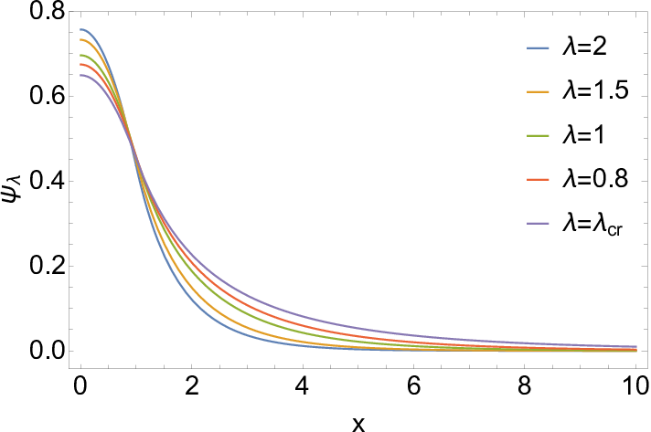
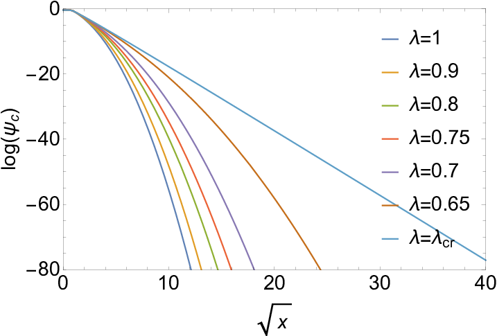
Using our theorem, we obtain for large and the following upper bound for the ground state of
In the subcritical case, the first part of the exponent corresponds to exponential fall-off and the second one is the polynomial correction since . As , the ground state energy approaches and the behavior of the ground state changes to
See Figure 3 for an illustration. A matching lower bound
can be obtained using a Comparison LemmaHoffmann-Ostenhof 1980a. Explicit calculations show that the eigenfunction has asymptotic behavior in the form
which is in perfect agreement with our result.
Our second example illustrates how the existence/non-existence of ground states at critical couplings depends on the dimensionHundertmark et al.. For this we need the notion of a nonnegative operator, i.e., , if for all functions in the domain of . Equivalently, the spectrum of , the set of allowed energies of the quantum system, is a subset of . In addition, we say a potential is critical, if but, for any nonnegative function which is not identically zero, the perturbed operator has a negative bound state.
In the following, let be nonnegative.
Theorem 2 (Non-existence of ground states at the ionization threshold).
does not have a ground state with energy if for some and all one has
Complementary to that
Theorem 3 (Existence of ground states at the ionization threshold).
has a ground state with energy if is a critical potential and, for some and all , one has
for .
Note that is positive if , zero if , and negative if . Hence, in dimensions the potential has to have a positive tail to support a ground state at the ionization threshold, whereas in dimensions it can be negative.
To illustrate this, let be a simple potential well, i.e.,
and consider the perturbed Hamiltonian
. It is well-known that always has a bound state below the ionization threshold in dimension Reed and Simon 1978. Whereas in dimensions the coupling has to be big enough in order to have a ground state below zeroReed and Simon 1978. If decreases from large values, there will be a critical value for which the ground state energy is zero. The question then is whether the ground state survives or disappears at . Our theorems above show that this depends crucially on the dimension. If the ground state survives, whereas in dimensions it disappears.
Atoms are described by the atomic Hamiltonian
where corresponds to the position of the nucleus and are the positions of electrons. We are using atomic units, i.e., , , , and . For convenience, we restrict to Born-Oppenheimer approximationBorn and Oppenheimer 1927, i.e., a nucleus of infinite mass fixed at ,
| (3) |
However, our results also hold for the operator without this approximationHundertmark et al. 2019a. We denote the ground state energy of by . In the first part, we saw that the asymptotic behavior in the critical case is controlled by the repulsive part of the potential. For atoms there are effectively two regions with different behavior.
Helium For , we introduce for and the region
where is the distance between the nucleus and the further away electron and is the distance of the closer electron to the nucleus. We note that for the special case we require . Roughly speaking, in the region we do not see the effective long range repulsion in and outside of the region we see only effective long range repulsion in . This corresponds to the intuitive explanation that the electron closer to the nucleus shields it from the second electron. Inside and outside of the region we get the following lower bound for the potential from Eq. (3) with :
Using these estimates we can bound the action of the operator (3) on a function supported inside and a function supported outside . More precisely, inside the region we can bound the kinetic energy of the electrons by zero and obtain a lower bound that depends only on and . Outside of we have to deal with a potentially singular term since is no longer bounded away from zero. However, we can bound this term with help of the corresponding kinetic energy term from below by . Plugging these estimates into the energy estimate, we can show that is positive provided that the function is chosen correctly in the two regions. In particular, we can prove for constants and the following asymptotic behavior of an eigenstate at the threshold:
Theorem 4.
A ground state of falls off faster than
in the interior of the region and faster than
outside of .
It is important to note that the constant holds only for . In the critical case , the constant becomes which forces to be sufficiently small, namely, . Moreover, the second critical case has a constant , where . The main ingredients in the proof are again an application of IMS localization formula and a clever choice of cutoff functions to separate the coordinate space into manageable regions Hundertmark et al. 2019a.
The lower bound for the Helium atom can be constructed in the same way as for one-particle model using Comparison Lemma. Unfortunately, we are only able to construct worse bounds compared to the one-particle case. In particular, we construct two lower bounds. The first one provides an exponential lower bound everywhere. The second one yields a subexponential lower bound outside of the regions and . The main difficulty in the construction of subsolutions for the operator (3) are singularities of the function . These can be remedied by a polynomial correction term Hoffmann-Ostenhof 1980b at the cost of a faster exponential fall-off constant. For a positive ground state function of the operator Eq. (3) such that and suitable constants , we obtain for every that satisfies
where the polynomial correction is given by
for suitably chosen function . However, the issue with the singularities is only present within the region . Therefore, we can derive a much better lower bound outside of that region.
Theorem 5.
For every s.t. the ground state of satisfies
where and
Thus, inside of the region, in which intuitively one electron shields the nucleus from the other one, we obtain comparable lower and upper bounds. We note that for we have .
General atom The procedure and the result for the upper bound can be generalized for an arbitrary atom with electrons. The main idea, i.e., construct two regions and estimate the action of the operator within, remains the same since there are still two regions with different asymptotic behavior. In the first one, all electrons are far away from the nucleus and the wavefunction falls off like an exponential function. In the second region, at least electrons remain relatively close to the nucleus while the other electrons can move far away. In this case, the outmost electrons are still bound but the wavefunction asymptotically behaves subexponentially. The physical mechanism for this confinement is not the attraction to the nucleus, which gets shielded by the inner electrons anyway, but the remaining long-range repulsion which acts as an effective barrier that prevents the system to break up. Hence, at least a stretched exponential fall-off persists.
Let be the ground state energy of an -electron atom of nuclear charge . Unlike the 2 electron Helium type system, it can now happen that more than one electron can be removed without energy cost: we assume the existence of a critical coupling such that
Thus the binding energy of electrons to the nucleus is equal to , but the binding energy of the -th electron is positive. Under the condition it was proved that a ground state existsGridnev and Garcia 2007. While this seems to be a reasonable assumptionHogreve 1998a; Sergeev and Kais 1999, it is not rigorously known. We considerably strengthen the previously known resultsGridnev and Garcia 2007; Bellazzini et al. 2014 by establishing much better bounds on the fall-off of the ground state eigenfunction at critical charge.
For simplicity, we consider only the case where each electron can uniquely be identified by its distance to the nucleus, i.e.
where gives the -th smallest value out of the distances of the electrons. This is not a real restriction. It is equivalent to omitting a set of measure which can be treated rigorously Hundertmark et al. 2019b. Due to this simplification we can introduce unique coordinates such that for each fixed point we have . One can now easily write the regions and estimates needed for our method. A detailed exposition of the derivation is given in the supplementary material. The final estimate which is needed in the proof of the claim can be summarized as
where
Note that describes the interaction between a nucleus and “inner” electrons including interactions between them. The expressions are in spirit the same as in the case of Helium. In particular, for a function supported within the region , the action of the operator is bounded from below by . Moreover, in the second region we obtain a positive lower bound for the action that depends on the distance of the outer coordinates to the nucleus. To summarize:
Theorem 6.
There exists a small enough and suitable constants such that a ground state of falls off like
if and like
otherwise.
The proofHundertmark et al. 2019b again reveals a distinct relation
between the repulsive part of the potential and the asymptotic behavior
of the eigenfunction similar to the one-particle model and also the two-particle (Helium) case.
In summary, we have shown, that existence and fall-off behavior of eigenfunctions at the critical coupling, for the class of operators (1),
depend on the asymptotic behavior of the potential. This was conjectured by quantum chemists.Hogreve 1998b
We also provided explicit, dimension-dependent conditions for the potential under which a zero-energy ground states does, or does not, exist.
We demonstrated how to apply our method to atomic systems under the additional assumption that , where is the critical charge of the nucleus, is the total number of electrons, and is the number of electrons leaving the atom as decreases below . It does not require any symmetry restriction on the quantum particles. This means that our result is valid for any statistics imposed on the electrons in atoms. In a real physical system, electrons are fermions, which means that the ground state for more than 2 electrons can not be strictly positive anymore. This unfortunately implies that we can not use Comparison Lemma to obtain a lower bound. It is necessary to find a different approach for systems with more than 2 electrons.
We only considered nonrelativistic quantum systems. For very large atoms, it is undoubtedly necessary to use, at least for the inner electrons, the corresponding relativistic equations to obtain the correct results. Our method relies mainly on the IMS localization formula. Thus using known results for pseudo-relativistic quantum systemsBarbaroux et al. 2019, it should be possible to to adapt our method to systems with pseudo-relativistic electrons.
Calculations suggest that similar results are valid within Hartree-Fock and Density Functional Theory (DFT). This is especially interesting due to the fact that these theories are inherently nonlinear. This would rigorously prove the asymptotic behavior predicted by various DFT-methodsGrabowski and Burke 2015. Another open problem is the applicability of our method for the case of interacting systems of multiple atoms, i.e., molecules. The additional geometry, due to the relative positions of the multiple atoms, as well as a more complicated relation between energy and electron distribution make this a hard to tackle but also a very interesting problem.
Acknowledgements.
Dirk Hundertmark was funded by the Deutsche Forschungsgemeinschaft (DFG, German Research Foundation) – Project-ID 258734477 – SFB 1173. Michal Jex received financial support from the Ministry of Education, Youth and Sport of the Czech Republic under the Grant No. RVO 14000. The work of Markus Lange was supported by NSERC of Canada.References
- von Neumann and Wigner (1993) J. von Neumann and E. P. Wigner, in The Collected Works of Eugene Paul Wigner (Springer, 1993) pp. 291–293.
- Agmon (1982) S. Agmon, Lectures on exponential decay of solutions of second-order elliptic equations: bounds on eigenfunctions of -body Schrödinger operators, Mathematical Notes, Vol. 29 (Princeton University Press, Princeton, 1982) p. 118.
- Hogreve (1995) H. Hogreve, Physics Letters A 201, 111 (1995).
- Dubau and Ivanov (1998) J. Dubau and I. A. Ivanov, Journal of Physics B: Atomic, Molecular and Optical Physics 31, 3335 (1998).
- Sergeev and Kais (2001) A. V. Sergeev and S. Kais, International Journal of Quantum Chemistry 82, 255 (2001).
- Estienne et al. (2014) C. S. Estienne, M. Busuttil, A. Moini, and G. W. F. Drake, Phys. Rev. Lett. 112, 173001 (2014).
- Gridnev and Garcia (2007) D. K. Gridnev and M. E. Garcia, J. Phys. A 40, 9003 (2007).
- Zhislin (1960) G. M. Zhislin, Trudy Moskovskogo matematiceskogo obscestva 9, 81 (1960).
- Lieb (1984) E. H. Lieb, Phys. Rev. A 29, 3018 (1984).
- Bethe (1929) H. Bethe, Zeitschrift für Physik 57, 815 (1929).
- Baker et al. (1990) J. D. Baker, D. E. Freund, R. N. Hill, and J. D. Morgan III, Physical Review A 41, 1247 (1990).
- Hoffmann-Ostenhof et al. (1983) M. Hoffmann-Ostenhof, T. Hoffmann-Ostenhof, and B. Simon, J. Phys. A 16, 1125 (1983).
- Hoffmann-Ostenhof and Hoffmann-Ostenhof (1984) M. Hoffmann-Ostenhof and T. Hoffmann-Ostenhof, J. Phys. A 17, 3321 (1984).
- Bellazzini et al. (2014) J. Bellazzini, R. L. Frank, E. H. Lieb, and R. Seiringer, Rev. Math. Phys. 26, 1350021, 18 (2014).
- Hogreve (1998a) H. Hogreve, Journal of Physics B: Atomic, Molecular and Optical Physics 31, L439 (1998a).
- Uchiyama (1969) J. Uchiyama, Publications of the Research Institute for Mathematical Sciences 5, 51 (1969).
- Persson (1960) A. Persson, Mathematica Scandinavica 8, 143 (1960).
- Cycon et al. (1987) H. L. Cycon, R. G. Froese, W. Kirsch, and B. Simon, Schrödinger operators with application to quantum mechanics and global geometry, study ed., Texts and Monographs in Physics (Springer-Verlag, Berlin, 1987) pp. x+319.
- Griesemer (2004) M. Griesemer, Journal of Functional Analysis 210, 321 (2004).
- Ismagilov (1961) R. S. Ismagilov, Dokl. Akad. Nauk SSSR 140, 33 (1961).
- Morgan (1979) J. D. Morgan, III, J. Operator Theory 1, 109 (1979).
- Sigal (1982) I. M. Sigal, Comm. Math. Phys. 85, 309 (1982).
- Hundertmark and Lee (2012) D. Hundertmark and Y.-R. Lee, J. Nonlinear Sci. 22, 1 (2012).
- Hundertmark et al. (2019a) D. Hundertmark, M. Jex, and M. Lange, arXiv:1908.04883 , 25 (2019a).
- Aizenman and Simon (1982) M. Aizenman and B. Simon, Comm. Pure Appl. Math. 35, 209 (1982).
- Hoffmann-Ostenhof (1980a) T. Hoffmann-Ostenhof, J. Phys. A 13, 417 (1980a).
- (27) D. Hundertmark, M. Jex, and M. Lange, to appear soon .
- Reed and Simon (1978) M. Reed and B. Simon, Methods of modern mathematical physics. IV. Analysis of operators (Academic Press, New York-London, 1978) pp. xv+396.
- Born and Oppenheimer (1927) M. Born and R. Oppenheimer, Annalen der Physik 389, 457 (1927).
- Hoffmann-Ostenhof (1980b) T. Hoffmann-Ostenhof, Phys. Lett. 77A, 140 (1980b).
- Sergeev and Kais (1999) A. V. Sergeev and S. Kais, International journal of quantum chemistry 75, 533 (1999).
- Hundertmark et al. (2019b) D. Hundertmark, M. Jex, and M. Lange, arXiv:1908.05016 , 14 (2019b).
- Hogreve (1998b) H. Hogreve, Physica Scripta 58, 25 (1998b).
- Barbaroux et al. (2019) J.-M. Barbaroux, M. Hartig, D. Hundertmark, and S. Vugalter, arXiv:1902.09222 , 47 (2019).
- Grabowski and Burke (2015) P. E. Grabowski and K. Burke, Physical Review A 91, 032501 (2015).
Supplementary material
Lower bound estimate In order to prove our theorem in general setting we need to be able to estimate the potential
from below in a suitable fashion. For this purpose we introduce the notion of inner and outer electrons as well as an ordering for the electrons. For simplicity we consider only the case where each electron can uniquely be identified by its distance to the nucleus, i.e.
where give the -th smallest value out of the distances of the electrons.We introduce unique coordinates such that for each fixed point we have .
We call the set
the inner coordinates and the set
the outer coordinates.
Moreover the potential corresponding to the most inner electrons is denoted by
We begin estimating the potential similar to the two electron case
where we used and within and outside . Provided that we split as follows
This process can be repeated for each inner coordinate, i.e. times. The last step yields
In the case that more than one electron leaves, i.e. , we can repeat the above procedure for all the remaining outer electrons.
The final estimate in the two resulting regions can be summarized as
Numerical examples: In the following we present additional examples of the asymptotic behavior for one-particle models. We consider again the operator describing a quantum particle in a potential well with a Coulomb repulsion term everywhere outside that well
| (4) |
However we do not decrease the depth of the well but increase the repulsion term. Due to the increase of the repulsive term outside the eigenfunctions become more localized for where is the numerically calculated critical value, see Figure 4.
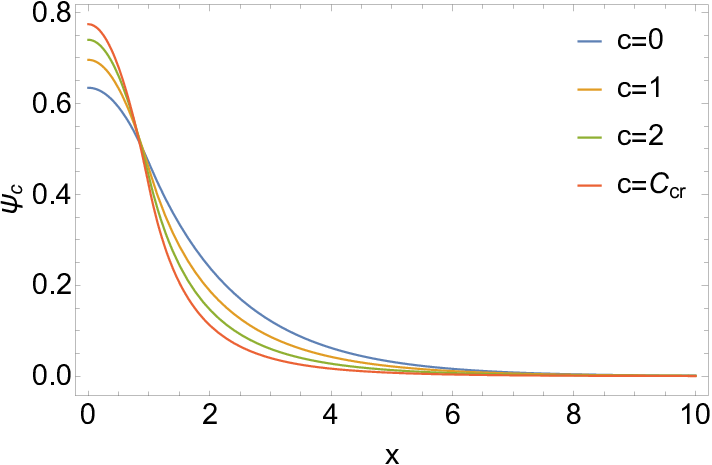

In order to emphasis that it is crucial to have a long range repulsive term we now consider the following Hamiltonian
| (5) |
The repulsive potential is present only in a finite region around the potential well. Note that the value is artificial and has no particular importance. If we start to increase the parameter up to the critical value we see that far away from the critical value the increase of leads to the localization of the wavefunction even by a short range potential. However for the wavefunction starts to spread further and further and for the fall-off of the function is hardly visible, see Figure 5.
The presented plots highlight the physical intuition that the wavefunction has to tunnel through the repulsive barrier in order to leave the potential well and delocalize.
However the long range Coulomb repulsion is too ’sticky’ for the wavefunction to delocalize even at the critical value and hence we are able to prove fall-off behavior at the ionization threshold.
Depiction of fall-off regions for Helium Atom In order to give the reader a better understanding of the fall-off behavior at the threshold and in particular to illustrate the respective sizes of the different regions we plot the ground state behavior for Helium in the case .
Figures 6 and 7 show that the exponential fall-off is almost everywhere. Only in the case that one of the electrons is close to the nucleus in comparison to the other one we obtain subexponential fall-off. This is due to the remaining long-range repulsion which acts as an effective barrier that prevents the system to break up. Figures 6 and 7 seem at the first glance similar. However the asymptotic behavior is significantly different. Volume of the amber cones grows as for the case of Figure 6 and as for the case of Figure 7.


The embedded graph is the zoomed in rectangular sector near the in -axis.
The difference is not so pronounced in the small region depicted however re-plotting the same regions in logarithmic scale in Figures 9 and 9 we see the dramatic difference for large values of .

