Adaptive Radar Detection and Classification Algorithms for Multiple Coherent SignalsThanks: Sudan Han is with the National Innovation Institute of Defense Technology, Beijing, China. E-mail: xiaoxiaosu0626@163.com.Thanks: Pia Addabbo is with Università degli studi “Giustino Fortunato”, Benevento, Italy. E-mail: p.addabbo@unifortunato.eu.Thanks: Linjie Yan, Yuxuan Zhang, and Chengpeng Hao are with Institute of Acoustics, Chinese Academy of Sciences, Beijing, China. E-mail: yanlinjie16@163.com; zhangyuxuan@mail.ioa.ac.cn; haochengp@mail.ioa.ac.cn.Thanks: Danilo Orlando is with the Engineering Faculty of Università degli Studi “Niccolò Cusano”, via Don Carlo Gnocchi 3, 00166 Roma, Italy. E-mail: danilo.orlando@unicusano.it.

In recent years, radar systems have become ubiquitous in real life due to the advances in digital architectures and miniaturization technologies. More importantly, the huge amount of computational power has paved the way for sophisticated processing algorithms fed by digital samples and leading to new architectures where the presence of analog hardware resources devoted to a specific task is very limited [1, 2, 3]. As a consequence, modern radar systems are extremely flexible and can incorporate different functions without additional hardware components.

In system design, the turning point is represented by the knocking down of high-frequency sampler and processing board costs that have allowed the development of fully-digital architectures. In this evolving scenario, radar research community continues to devise algorithms with increased complexity that take full advantage of the potential provided by digital architectures. The quid pro quo of the increased computational power is represented by the enhanced performance as corroborated, for instance, by the space and/or time adaptive algorithms developed in the open literature. As a matter of fact, focusing on the radar detection task and starting from the seminal works by Kelly [4, 5], a plethora of decision schemes have been proposed by enriching the design assumptions in order to account for a priori information and/or specific aspects of the application/system under consideration [6, 4, 7, 8, 9, 10, 11, 12, 13, 14, 15, 16, 17, 18, 19, 20].

It is also important to underline that the benefits coming from the aforementioned technology advances have been also exploited by the Electronic Warfare (EW) systems, which have adapted themselves to the more and more reliable capabilities of radar systems leading to a more effective class of electronic countermeasures referred to as smart jammers [21, 3, 22, 23, 24, 25]. For instance, modern noise-like jamming systems are capable of transmitting narrow-band interfering signals which are concurrent with the radar pulses according to the radar pulse repetition interval after having estimated it (EW integrated systems). Moreover, they can use an intrapulse modulation to generate a noise bandwidth at radio frequency, while maintaining phase coherence over a group of successive jamming pulses [25]. Remarkably, this kind of jammers can generate signals that are coherent (i.e., fully correlated) with the desired signal even though the former impinge on the radar from different directions [26, 27]. An analogous situation occurs in scenarios where, due to multipath propagation, replicas of the original signal come back to the receiver with a sufficiently small delay difference [27, 28].

The main drawback caused by the presence of multiple coherent signals is that they can completely destroy the performance of the most common high-resolution direction finding algorithms for adaptive array systems [29, 30]. As a matter of fact, coherent signals appear as a single signal impinging on the array of sensors and that, more importantly, arrives from a direction which is quite different from that of the sought signals. As a consequence, high-resolution eigenstructure-based techniques as, for instance, MUltiple SIgnal Classification algorithm [29], fail to correctly resolve the signals jeopardizing the Angle of Arrival (AoA) estimation [26]. Similar remarks also hold for another important approach to AoA estimation, namely the CLEAN algorithm [31] which consists in iterative cancellations of strong signals under the assumption that the spatial covariance matrix results from the sum of contributions associated with uncorrelated sources. Remarkably, it can be used for the detection of weak targets embedded in strong interference signals [32, 33, 34].

In order to mitigate the effects of coherent signals, data feeding the direction finding algorithm can be suitably preprocessed in order to decrease the correlation of the impinging signals. In this respect, spatial smoothing technique [30] combines data obtained from synthetic subarrays whose size is lower than that of the original array with the drawback of a reduced angular resolution. In the context of subspace-based algorithms, in [35] a method based upon the weighted subspace fitting criterion is proposed to jointly detect and estimate the number and the related parameters of the coherent signals. However, this method does not allow for the control of the probability of false alarm ($P_{fa}$) which is of primary concern in radar. Alternative approaches against the coherent signals problem can rely on the Maximum Likelihood (ML) estimation [36] which, however, is computationally intensive and requires the knowledge of the number of coherent signals, or the compressed sensing paradigm where a further stage for estimate fusion is required [37, 38].

Thus, in order to save computational resources (due to the activation of additional processing stages also in situations where they are not required) and to take advantage of the full angular resolution of the system, a detection stage capable of deciding for the presence of a target and possible coherent signals by estimating, as a byproduct, their number along with other side information is highly desirable. In fact, when this stage declares the presence of noncoherent signals, direction finding algorithms can be applied without losses in resolution. On the other hand, when coherent signals are present, the rough estimates of the corresponding parameters provided by this stage can be used to drive ML-based direction finding algorithms to reduce their computational load. Remarkably, such stage can be viewed as an Electronic Counter-CounterMeasure.

With the above remarks in mind, in this paper we devise a detection architecture accounting for the presence of coherent signals and that can provide an estimate of their number as well as the AoAs. To this end, at the design stage, we formulate the problem at hand in terms of a multiple hypothesis test, comprising the usual null (or interference-only) hypothesis, the conventional signal-plus-interference hypothesis, and multiple alternative hypotheses that differ in the number of coherent echoes. These signals are assumed to follow Swerling II Target Model, which assumes that the Radar Cross Section (RCS) of the target obeys the chi-squared distribution with two degrees of freedom [1]. Then, assuming an upper bound on the number of impinging signals (that can be dictated by system parameters), we conceive likelihood-ratio-based decision rules which exploit suitable penalty terms borrowed from the Model Order Selection (MOS) rules [39, 40]. Therefore, the proposed architectures can provide an estimate of the actual number of coherent signals. As for the AoA estimation, the angular sector under consideration is sampled to form a discrete set of angular positions that are used at the design stage. Besides, since the exhaustive search can become very time demanding for high numbers of signals, we design a suboptimum iterative procedure providing satisfactory performance at least for the considered numerical examples. Finally, the performance assessment is conducted over synthetic data in comparison with classical detection architectures and highlights that the proposed schemes represent an effective means to face with the problem of target detection in the presence of coherent signals.

The remainder of the paper is organized as follows. Section II is devoted to problem formulation and the definitions used in the next derivations, while the design of the detection and estimation architectures is described in Section III. Section IV shows the effectiveness of the proposed strategies through numerical examples on simulated data. Finally, Section V contains concluding remarks and charts a course for future works.

Let us assume that a search radar system is equipped with a uniform linear array with $N$ antennas and transmits $L$ pulses in the nominal beam position during one scan cycle. Then, each antenna collects $L$ samples from the cell under test. Denote by ${\mbox{\boldmath$z$}}_{l}\in{\mathds{C}}^{N\times 1}$, $l=1,\ldots,L$, the vector whose entries are the $l$th returns from each antenna and by ${\mbox{\boldmath$Z$}}_{L}=[{\mbox{\boldmath$z$}}_{1},\ldots,{\mbox{\boldmath$z$}}_{L}]\in{\mathds{C}}^{N\times L}$ the overall data matrix, the classical radar detection problem consists in deciding whether or not ${\mbox{\boldmath$Z$}}_{L}$ contains the target of interest, namely, a component whose signature coincides with the nominal steering vector. Before proceeding with the problem formulation, it is important to state here that the columns of ${\mbox{\boldmath$Z$}}_{L}$ are assumed statistically independent and, hence, temporally noncoherent, whereas each column is representative of both spatially correlated clutter and spatially coherent useful signal components (a point better explained below).

As customary, we assume that a set of $K$ ($K\geq N$) secondary data, ${\mbox{\boldmath$z$}}_{k}\in{\mathds{C}}^{N\times 1}$, $k=1,\ldots,K$, free of target components and sharing the same statistical properties of the interference in the cell under test, is available [4, 7, 12, 41]. Under the above assumptions, this problem can be formulated in terms of a conventional binary hypothesis test whose expression is (see [4, 7, 12] and references therein)

where

• •

  ${\mbox{\boldmath$n$}}_{l},{\mbox{\boldmath$n$}}_{k}\sim\mbox{$\mathcal{C}$}\mbox{$\mathcal{N}$}_{N}({\mbox{\boldmath$0$}},{\mbox{\boldmath$M$}})$, $l=1,\ldots,L$, $k=1,\ldots,K$, are IID with unknown positive definite covariance matrix ${\mbox{\boldmath$M$}}\in{\mathds{C}}^{N\times N}$ representative of the thermal noise plus clutter; $M$ is referred to in the following as Interference Covariance Matrix (ICM);

• •

  $\alpha_{1},\ldots,\alpha_{L}\sim\mbox{$\mathcal{C}$}\mbox{$\mathcal{N}$}_{1}(0,\sigma_{\alpha}^{2})$ with $\sigma_{\alpha}^{2}>0$ are IID random variables accounting for both the target response (RCS) and channel effects (Swerling II target model [1]);

• •

  ${\mbox{\boldmath$v$}}(\theta_{t})\in{\mathds{C}}^{N\times 1}$ is the nominal (spatial) steering vector whose expression is

  $${\mbox{\boldmath$v$}}(\theta_{t})\!\!=\!\![1,\exp\{j\pi\sin(\theta_{t})\},\ldots,\exp\{j\pi(N-1)\sin(\theta_{t})\}]^{T}\!\!,$$

  where $\theta_{t}$ is the (known) AoA of the target measured with respect to the array broadside and we have assumed that the inter-element spacing is half the operating wavelength in order to avoid the aliasing of the spatial frequency.

However, as stated in Section I, in practical applications the generic ${\mbox{\boldmath$z$}}_{l}$ might not only contain the direct echo but also returns from other directions and that, more importantly, are coherent (i.e., fully correlated) with the former due, for instance, to the effects of multipath propagation and/or the presence of smart jammers [26, 27, 28]. As a consequence, the conventional radar detection problem (1) consisting of two hypotheses may be no longer representative of the actual operating scenario. In fact, in such case, the alternative hypothesis can be replaced by the following

where $M$ is the actual number of coherent signals, which is unknown. However, notice that the uncertainty on $M$ naturally leads to multiple alternative hypotheses, $H_{1,i}$ say, which differ in the number of coherent signals. Therefore, assuming an upper bound, $M_{c}$ say, on the latter unknown parameter, a possible approach to account for the presence of possible fully-correlated signals consists in considering a multiple hypothesis test where besides the conventional $H_{0}$ and $H_{1}$ hypotheses, $M_{c}<N$ additional hypotheses¹¹ 1 The constraint $M_{c}<N$ is due to both the fact that $N$ degrees of freedom are required to estimate $N$ AoAs also making matrix ${\mbox{\boldmath$V$}}_{i}$, defined in (6), full-column rank., corresponding to scenarios containing a different number of coherent signals, appear. Therefore, problem (1) can be generalized as follows

$i=1,\ldots,M_{c}$, where the $\alpha_{l}$s, the ${\mbox{\boldmath$n$}}_{l}$s, and the ${\mbox{\boldmath$n$}}_{k}$s have been already defined for problem (1) and

• •

  $M_{c}\geq M$ is an upper bound on the number of coherent signals²² 2 Note that problem (3) reduces to (1) when $M_{c}=0$.;

• •

  given $i\in\{1,\ldots,M_{c}\}$ and $k\in\{1,\ldots,i\}$, the coefficients $\beta_{1,k},\ldots,\beta_{L,k}\in{\mathds{C}}$ are IID complex Gaussian random variables with zero mean and variance $\sigma_{k}^{2}>0$; they represent the complex amplitudes of the $k$th coherent signal over the time³³ 3 It is worth noticing that Swerling II target model is also adopted for the coherent signals.;

• •

  given $i\in\{1,\ldots,M_{c}\}$, $\theta_{1},\ldots,\theta_{i}$ are the unknown AoAs of the additional coherent signals.

Finally, we assume that, $\forall i=1,\ldots,M_{c}$, the random variables $\alpha_{l}$, $\beta_{l,1},\ldots,\beta_{l,i}$ are fully correlated. Otherwise stated, given $l\in\{1,\ldots,L\}$ and $i\in\{1,\ldots,M_{c}\}$, $\forall k,h\in\{1,\ldots,i\}$ and $k\neq h$ the following equalities hold

In order to unburden the notation, hereafter we omit the dependence of the steering vectors on the AoAs and denote by ${\mbox{\boldmath$v$}}_{t}$ the nominal steering vector whereas we use $\mbox{\boldmath$p$}_{i}$ to indicate the steering vector associated with the coherent signal whose AoA is $\theta_{i}$.

Before concluding this section, we provide some definitions that will come in handy for the next developments. More precisely, the PDF of ${\mbox{\boldmath$Z$}}_{L}$ under $H_{0}$ has the following expression

whereas its PDF under the generic $H_{1,i}$, $i=0,\ldots,M_{c}$, is given by

where ${\mbox{\boldmath$V$}}_{i}=[{\mbox{\boldmath$v$}}_{t},\mbox{\boldmath$p$}_{1},\ldots,\mbox{\boldmath$p$}_{i}]\in{\mathds{C}}^{N\times(i+1)}$ and ${\mbox{\boldmath$R$}}_{i}={\mathbb{E}}[{\mbox{\boldmath$\nu$}}_{l,i}{\mbox{\boldmath$\nu$}}_{l,i}^{\dagger}]\in{\mathds{C}}^{(i+1)\times(i+1)}$, $l=1,\ldots,L$, with ${\mbox{\boldmath$\nu$}}_{l,i}=[\alpha_{l},\beta_{l,1},\ldots,\beta_{l,i}]^{T}\in{\mathds{C}}^{(i+1)\times 1}$. It is understood that when $i=0$, ${\mbox{\boldmath$V$}}_{0}$ and ${\mbox{\boldmath$\nu$}}_{l,0}$ coincide with ${\mbox{\boldmath$v$}}_{t}$ and $\alpha_{l}$, respectively.

In this section, we devise a detection architecture for problem (3) that relies on a penalized log-likelihood ratio test [29, 42] whose generic structure is given by

where

$\eta$ is the detection threshold to be set according to a desired⁴⁴ 4 Hereafter, we denote by $\eta$ the generic detection threshold. $P_{fa}$,

with⁵⁵ 5 Notice that for $i=0$, the maximization at the numerator of (9) is with respect to $\sigma^{2}_{\alpha}$ only. $\widehat{{\mbox{\boldmath$M$}}}$ a suitable estimate of $M$, and $c\cdot h(i)$ is a penalty term borrowed from the MOS rules [39] with $h(i)$ the number of unknown real-valued parameters under the $H_{1,i}$ hypothesis and $c$ a suitable scaling factor. Specifically, $c$ can be set according to the Akaike Information Criterion (AIC), Bayesian Information Criterion (BIC), and Generalized Information Criterion (GIC), namely

Two important remarks are now in order. First, notice that $\widehat{\Lambda}_{i}({\mbox{\boldmath$Z$}}_{L})$ is the logarithm of a decision statistic obtained by resorting to a modified Generalized Likelihood Ratio Test (GLRT)-based design procedure [7], where the ICM is firstly assumed known and then replaced by an estimate. In the specific case, we use the ML estimate based upon the training samples only (namely, the sample covariance matrix that is invertible with probability $1$ since $K\geq N$), whose expression is⁶⁶ 6 This design choice is dictated by the fact that deriving closed-form expression for the plain GLRT is not mathematically tractable at least to the best of authors’ knowledge.

Second, the correlation of the signals makes the columns of the positive semidefinite matrix ${\mbox{\boldmath$R$}}_{i}$ proportional. Therefore, the resulting rank is $1$ and it can be factorized as

where ${\mbox{\boldmath$r$}}_{i}\in{\mathds{C}}^{(i+1)\times 1}$. As a consequence, the number of unknown real-valued parameters under $H_{1,i}$ can be written as $h(i)=N^{2}+1+2i$. With the above remarks in mind, let us proceed by deriving $\widehat{\Lambda}_{0}({\mbox{\boldmath$Z$}}_{L})$, namely

Applying the Woodbury identity [43], we come up with the following expression

where ${\mbox{\boldmath$v$}}_{w}={\mbox{$\widehat{{\mbox{\boldmath$M$}}}$}}^{-1/2}{\mbox{\boldmath$v$}}_{t}$ and ${\mbox{\boldmath$S$}}_{w}={\mbox{$\widehat{{\mbox{\boldmath$M$}}}$}}^{-1/2}{\mbox{\boldmath$Z$}}_{L}{\mbox{\boldmath$Z$}}_{L}^{\dagger}{\mbox{$\widehat{{\mbox{\boldmath$M$}}}$}}^{-1/2}$. Let us define the function

and observe that $\lim_{\sigma^{2}_{\alpha}\rightarrow 0}g_{0}(\sigma^{2}_{\alpha})=0$ and $\lim_{\sigma^{2}_{\alpha}\rightarrow+\infty}g_{0}(\sigma^{2}_{\alpha})=-\infty$. Thus, in order to maximize $g_{0}(\sigma^{2}_{\alpha})$, we find the zeros of its first derivative with respect to $\sigma_{\alpha}^{2}$ to obtain

Moreover, $g_{0}(\sigma^{2}_{\alpha})$ is monotonic increasing when $\sigma^{2}_{\alpha}<({{\mbox{\boldmath$v$}}_{w}^{\dagger}{\mbox{\boldmath$S$}}_{w}{\mbox{\boldmath$v$}}_{w}-L\lVert{\mbox{\boldmath$v$}}_{w}\rVert^{2}})/({L\lVert{\mbox{\boldmath$v$}}_{w}\rVert^{4}})$ and decreasing for $\sigma^{2}_{\alpha}>({{\mbox{\boldmath$v$}}_{w}^{\dagger}{\mbox{\boldmath$S$}}_{w}{\mbox{\boldmath$v$}}_{w}-L\lVert{\mbox{\boldmath$v$}}_{w}\rVert^{2}})/({L\lVert{\mbox{\boldmath$v$}}_{w}\rVert^{4}})$ (provided that ${\mbox{\boldmath$v$}}_{w}^{\dagger}{\mbox{\boldmath$S$}}_{w}{\mbox{\boldmath$v$}}_{w}>L\lVert{\mbox{\boldmath$v$}}_{w}\rVert^{2}$). As a consequence, (16) represents a maximum point of $g_{0}(\sigma^{2}_{\alpha})$. It follows that (14) can be recast as

The next step towards the computation of (7) consists in deriving $\widehat{\Lambda}_{i}({\mbox{\boldmath$Z$}}_{L})$ for $i=1,\ldots,M_{c}$. To this end, observe that

Replacing (12) into the most right-hand side of the above equation and applying the Woodbury identity leads to

where ${\mbox{\boldmath$V$}}_{w,i}={\mbox{$\widehat{{\mbox{\boldmath$M$}}}$}}^{-1/2}{\mbox{\boldmath$V$}}_{i}$ and ${\mbox{\boldmath$S$}}_{w}$ has been previously defined. Since ${\mbox{\boldmath$V$}}_{i}$ has a Vandermonde structure and $\widehat{{\mbox{\boldmath$M$}}}$ is nonsingular, also matrices ${\mbox{\boldmath$A$}}_{i}={\mbox{\boldmath$V$}}_{w,i}^{\dagger}{\mbox{\boldmath$V$}}_{w,i}$ and ${\mbox{\boldmath$B$}}_{i}={\mbox{\boldmath$V$}}_{w,i}^{\dagger}{\mbox{\boldmath$S$}}_{w}{\mbox{\boldmath$V$}}_{w,i}$ are nonsingular and (19) can be expressed in terms of these matrices as

Exploiting the Cholesky decomposition of ${\mbox{\boldmath$A$}}_{i}$, given by

where ${\mbox{\boldmath$C$}}_{i}\in{\mathds{C}}^{(i+1)\times(i+1)}$ is a lower triangular matrix, the right-hand side of (20) can be recast as

where

As further step towards the solution of the above problem, we decompose ${\mbox{\boldmath$a$}}_{i}$ as the product of a positive scalar $\sqrt{a_{i}}$, with $a_{i}>0$, times a unit-norm vector ${\mbox{\boldmath$u$}}_{a,i}$. Thus, problem (22) is tantamount to

Denoting by

the maximization with respect to $a_{i}$ can be performed by investigating the behavior of $g(a_{i})$ over the interval $(0,+\infty)$. Specifically, since the following equalities hold

we can search for the stationary points of $g(a_{i})$ in the interior of its domain by setting to zero its first derivative with respect to $a_{i}$ to obtain

Moreover, it is not difficult to show that $g(a_{i})$ is increasing when $a_{i}<({{\mbox{\boldmath$u$}}_{a,i}^{\dagger}{\mbox{\boldmath$D$}}_{i}{\mbox{\boldmath$u$}}_{a,i}-L})/{L}$ and decreasing in the opposite case (provided that ${\mbox{\boldmath$u$}}_{a,i}^{\dagger}{\mbox{\boldmath$D$}}_{i}{\mbox{\boldmath$u$}}_{a,i}>L$). As a consequence, (27) represents a maximum point. Now, plugging (27) into (24), the maximization problem can be recast as () at the bottom of this page.

The maximization over ${\mbox{\boldmath$u$}}_{a,i}$ can be conducted by defining the function $f(x)=x-L\log x+L\log L-L$, which is monotonic increasing for $x\geq L$. In fact, its first derivative is $\frac{df(x)}{dx}=1-\frac{L}{x}\geq 0$, $\forall x\geq L$. Therefore, the maximum of $f({\mbox{\boldmath$u$}}_{a,i}^{\dagger}{\mbox{\boldmath$D$}}_{i}{\mbox{\boldmath$u$}}_{a,i})$ with respect to ${\mbox{\boldmath$u$}}_{a,i}$ can be obtained by directly optimizing argument, i.e., ${\mbox{\boldmath$u$}}_{a,i}^{\dagger}{\mbox{\boldmath$D$}}_{i}{\mbox{\boldmath$u$}}_{a,i}$. Exploiting the Rayleigh-Ritz Theorem [43], we obtain that

and the maximum is attained when ${\mbox{\boldmath$u$}}_{a,i}$ is the normalized eigenvector of ${\mbox{\boldmath$D$}}_{i}$ corresponding to its maximum eigenvalue. Gathering the above results, we obtain () at the bottom of this page.

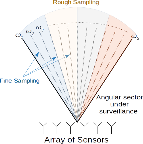
The last optimization problem to be solved is with respect to the AoAs of the coherent signals. In this respect, since deriving closed-form expressions for the ML estimates of $\theta_{1},\ldots,\theta_{i}$ represents a difficult task (at least to the best of authors’ knowledge), we devise grid-search methods. More precisely, the angular sector under surveillance is sampled to form a discrete set of angular positions which is denoted by $\Omega=\{\omega_{1},\ldots,\omega_{S}\}$ (see Figure 1). The cardinality of $\Omega$ can be chosen according to both the computational power available at the receiver and the system requirements in terms of reactivity time intervals. It is clear that a dense sampling of the angular sector increases the processing time but can provide better estimation results with respect to the case where the sampling interval is large. However, in the latter case, the computational load is lower than in the former case. Nevertheless, an iterative approach can be pursued for the maximization under the generic $H_{1,i}$ hypothesis and for each $i\in\{1,\ldots,M_{c}\}$. Specifically, given $i\in\{1,\ldots,M_{c}\}$ and assuming that $H_{1,i}$ holds true, we start by roughly sampling the angular sector of interest and use this search grid to come up with preliminary estimates of the assumed $i$ AoAs. Then, we use these estimates to identify a restricted angular sector (resulting from the union of partially overlapped narrow sectors) comprising suitable guard bands.

with the constraint that admissible candidates are such that $\omega_{1}\neq\omega_{2}\neq\ldots\neq\omega_{i}$. On the other hand, exhaustive grid search can be prohibitive for large $M_{c}$ values. In this case, in order to limit the number of operations, we design a suboptimum search method relying on the cyclic optimization paradigm [44]. Specifically, let us assume that $H_{1,i}$ is true and that $i-1$ estimates, $\widehat{\Theta}_{1,i}^{(0)}=\{\hat{\theta}^{(0)}_{2},\ldots,\hat{\theta}^{(0)}_{i}\}\subset\Omega$ say, are available, then we select $\theta_{1}\in\Omega$ exploiting the following criterion

where ${\mbox{\boldmath$D$}}_{i}(\theta_{1},\widehat{\Theta}_{1}^{(0)})$ is computed as ${\mbox{\boldmath$D$}}_{i}$ in (23) with the difference that ${\mbox{\boldmath$V$}}_{i}$ is replaced by the following matrix

The new estimate $\hat{\theta}_{1}^{(1)}$ is used to form $\widehat{\Theta}_{2,i}^{(0)}=\{\hat{\theta}^{(1)}_{1},\hat{\theta}^{(0)}_{3},\ldots,\hat{\theta}^{(0)}_{i}\}$ and the update of $\hat{\theta}_{2}$ is obtained as

where ${\mbox{\boldmath$D$}}_{i}(\theta_{2},\widehat{\Theta}_{2,i}^{(0)})$ is built up using

The above steps continue until the $i$th update occurs to obtain $\widehat{\Theta}_{1,i}^{(1)}=\{\hat{\theta}^{(1)}_{2},\ldots,\hat{\theta}^{(1)}_{i}\}$, which can be used to repeat the entire refinement procedure.

Summarizing, the update of the $k$th AoA within the $n$th ($n\geq 1$) procedure cycle has the following expression

$1\leq k\leq i$, where

and ${\mbox{\boldmath$D$}}_{i}(\theta_{k},\widehat{\Theta}_{k,i}^{(n-1)})$ is defined as in (23) with ${\mbox{\boldmath$V$}}_{i}\left(\theta_{k},\widehat{\Theta}_{k,i}^{(n-1)}\right)=[{\mbox{\boldmath$v$}}_{t},{\mbox{\boldmath$v$}}(\hat{\theta}_{1}^{(n)}),\ldots,{\mbox{\boldmath$v$}}(\hat{\theta}_{k-1}^{(n)}),{\mbox{\boldmath$v$}}(\theta_{k}),{\mbox{\boldmath$v$}}(\hat{\theta}_{k+1}^{(n-1)}),\ldots,{\mbox{\boldmath$v$}}(\hat{\theta}_{i}^{(n-1)})].$ It is important to observe that the above procedure leads to a nondecreasing sequence of log-likelihood function values, namely

where

The entire procedure may terminate when

where $\epsilon>0$, or $n\geq N_{\max}$ where $N_{\max}$ is the maximum allowable number of iterations.

Finally, as for the initialization of the procedure, given the received vectors, we proceed by first computing

then, sort the above values in decreasing order, namely

and select $\omega_{k_{1}},\ldots,\omega_{k_{i}}$. The behavior of the proposed architectures coupled with the above estimation procedure is assessed in the next section by means of numerical examples.

In this section, the performance of the proposed detection architectures is investigated drawing upon synthetic data and considering three operating scenarios. In the first case, only the target of interest is present, whereas in the second scenario, an additional coherent signal is considered. Finally, the third scenario contains the signal of interest along with two additional coherent signals. The performance metrics are

• •

  the Probability of Detection under $H_{1,i}$, $i\geq 0$, ($P_{d,i}$) defined as the probability of rejecting $H_{0}$ when the latter is false and given a preassigned $P_{fa}=P(\mbox{reject }H_{0}|H_{0}\mbox{ is true})$;

• •

  the Probability of Correct Classification ($P_{cc}$), namely the probability of deciding⁷⁷ 7 The detection threshold is set according to the preassigned $P_{fa}$ also in this case. for $H_{1,i}$ under $H_{1,i}$;

• •

  the Root Mean Square Error (RMSE) in angle whose expression is

  $$\sqrt{{\mathbb{E}}\left[\frac{1}{M}\sum_{m=1}^{M}\displaystyle\min_{k=1,\ldots,\hat{i}}\left\{(\theta_{m}-\hat{\theta}_{k})^{2}\right\}\right]},$$

  (43)

where $\hat{\theta}_{k}$, $k=1,\ldots,\hat{i}$, are the AoA estimates of the coherent signals when $H_{1,\hat{i}}$ is declared. Since deriving closed-form expressions for the above quantities represents a mathematically intractable task (at least to the best of authors’ knowledge), we estimate them resorting to the Monte Carlo counting techniques (also replacing the statistical expectation of the RMSE with the sample mean over the Monte Carlo trials). More precisely, we exploit $10^{3}$ independent trials to estimate the considered performance metrics, whereas the detection thresholds are set over $100/P_{fa}$, with $P_{fa}=10^{-3}$.

As stated before, the analysis starts from the conventional case where only the target echoes impinge on the radar and proceeds with two more difficult cases that assume the presence of two and three coherent signals (including that of interest), respectively. As for the operating setup, the coherent signals share the same power as the target signal, whereas the angular sector under surveillance ranges from $-25$ to $25$ degrees and is sampled at $1$ degree. The Signal-to-Interference-plus-Noise Ratio (SINR) is defined as $\mbox{SINR}=\sigma_{\alpha}^{2}{\mbox{\boldmath$v$}}_{t}^{\dagger}{\mbox{\boldmath$M$}}^{-1}{\mbox{\boldmath$v$}}_{t}$, where ${\mbox{\boldmath$M$}}=\sigma_{n}^{2}{\mbox{\boldmath$I$}}+\mbox{CNR}\,{\mbox{\boldmath$M$}}_{c}$, $\mbox{CNR}=20$ dB is the Clutter-to-Noise Ratio, $\sigma^{2}_{n}=1$ is the noise power, and ${\mbox{\boldmath$M$}}_{c}$ is the clutter covariance matrix whose $(i,j)$th entry is defined as ${\mbox{\boldmath$M$}}_{c}(i,j)=\rho_{c}^{|i-j|}$ with $\rho_{c}=0.9$ the one-lag correlation coefficient. Moreover, all the numerical examples assume $N=16$, $L=32$, $\theta_{t}=0^{\circ}$, and $M_{c}=4$.

As for the angular positions of the coherent signals, we begin the analysis assuming that they belong to the search grid. In this case, the obtained curves represent an upper bound on the performance that can be attained exploiting fine and fine search grids (possibly considering the previously described iterative maximization procedure). Then, we investigate the behavior of the proposed architectures when the actual positions of the coherent signals are in between the points of the search grid. Specifically, we generate them as uniformly distributed in intervals of different sizes and centered on the nominal search grid points (a point better explained below).

Finally, we compare the proposed architectures with well-known decision schemes, namely the Generalized Adaptive Matched Filter (GAMF) and the Generalized Adaptive Subspace Detector (GASD) given by [41]

References

- [1] M. A. Richards, J. A. Scheer, and W. A. Holm, Principles of Modern Radar: Basic Principles. Raleigh, NC: Scitech Publishing, 2010.
- [2] W. L. Melvin and J. A. Scheer, Principles of Modern Radar: Advanced Techniques, S. Publishing, Ed., Edison, NJ, 2013.
- [3] M. A. Richards, W. L. Melvin, J. A. Scheer, and W. A. Holm, Principles of Modern Radar: Radar Applications, Volume 3, ser. Electromagnetics and Radar. Institution of Engineering and Technology, 2013.
- [4] E. J. Kelly, “An adaptive detection algorithm,” IEEE Transactions on Aerospace and Electronic Systems, vol. 22, no. 2, pp. 115–127, 1986.
- [5] E. J. Kelly and K. Forsythe, “Adaptive Detection and Parameter Estimation for Multidimensional Signal Models,” Lincoln Lab, MIT, Lexington, US, Technical Report 848, 1989.
- [6] W. L. Melvin, “Space-time Adaptive Radar Performance in Heterogeneous Clutter,” IEEE Transactions on Aerospace and Electronic Systems, vol. 36, no. 2, pp. 621–633, 2000.
- [7] F. C. Robey, D. R. Fuhrmann, E. J. Kelly, and R. Nitzberg, “A CFAR adaptive matched filter detector,” IEEE Transactions on Aerospace and Electronic Systems, vol. 28, no. 1, pp. 208–216, 1992.
- [8] F. Gini and A. Farina, “Vector Subspace Detection in Compound-Gaussian Clutter Part I: Survey and New Results,” IEEE Transactions on Aerospace and Electronic Systems, vol. 38, no. 4, pp. 1295–1311, 2002.
- [9] D. Orlando and G. Ricci, “A Rao Test With Enhanced Selectivity Properties in Homogeneous Scenarios,” IEEE Transactions on Signal Processing, vol. 58, no. 10, pp. 5385–5390, 2010.
- [10] W. Liu, W. Xie, and Y. Wang, “Rao and Wald Tests for Distributed Targets Detection With Unknown Signal Steering,” IEEE Signal Processing Letters, vol. 20, no. 11, pp. 1086–1089, 2013.
- [11] Y. I. Abramovich and B. A. Johnson, “GLRT-based detection-estimation for undersampled training conditions,” IEEE Transactions on Signal Processing, vol. 56, no. 8, pp. 3600–3612, 2008.
- [12] F. Bandiera, D. Orlando, and G. Ricci, Advanced Radar Detection Schemes Under Mismatched Signal Models. San Rafael, US: Synthesis Lectures on Signal Processing No. 8, Morgan & Claypool Publishers, 2009.
- [13] W. Liu, W. Xie, J. Liu, and Y. Wang, “Adaptive Double Subspace Signal Detection in Gaussian Background—Part I: Homogeneous Environments,” IEEE Transactions on Signal Processing, vol. 62, no. 9, pp. 2345–2357, 2014.
- [14] W. Liu, J. Liu, Y. Gao, G. Wang, and Y. L. Wang, “Multichannel signal detection in interference and noise when signal mismatch happens,” Signal Processing, vol. 166, p. 107268, 2020.
- [15] J. Liu, S. Sun, and W. Liu, “One-step persymmetric GLRT for subspace signals,” IEEE Transaction on Signal Processing, vol. 14, no. 67, pp. 3639–3648, July 15 2019.
- [16] C. Hao, S. Gazor, G. Foglia, B. Liu, and C. Hou, “Persymmetric adaptive detection and range estimation of a small target,” IEEE Transactions on Aerospace and Electronic Systems, vol. 51, no. 4, pp. 2590–2604, 2015.
- [17] G. Foglia, C. Hao, A. Farina, G. Giunta, D. Orlando, and C. Hou, “Adaptive Detection of Point-Like Targets in Partially Homogeneous Clutter With Symmetric Spectrum,” IEEE Transactions on Aerospace and Electronic Systems, vol. 53, no. 4, pp. 2110–2119, 2017.
- [18] C. Hao, D. Orlando, G. Foglia, and G. Giunta, “Knowledge-Based Adaptive Detection: Joint Exploitation of Clutter and System Symmetry Properties,” IEEE Signal Processing Letters, vol. 23, no. 10, pp. 1489–1493, October 2016.
- [19] G. Foglia, C. Hao, G. Giunta, and D. Orlando, “Knowledge-aided adaptive detection in partially homogeneous clutter: Joint exploitation of persymmetry and symmetric spectrum,” Digital Signal Processing, vol. 67, no. Supplement C, pp. 131 – 138, 2017.
- [20] P. Wang, Z. Sahinoglu, M. Pun, and H. Li, “Persymmetric Parametric Adaptive Matched Filter for Multichannel Adaptive Signal Detection,” IEEE Transactions on Signal Processing, vol. 60, no. 6, pp. 3322–3328, 2012.
- [21] D. K. Barton, Radar Equations for Modern Radar, ser. Artech House radar library. Artech House, 2013.
- [22] D. J. Bachmann, R. J. Evans, and B. Moran, “Game Theoretic Analysis of Adaptive Radar Jamming,” IEEE Transactions on Aerospace and Electronic Systems, vol. 47, no. 2, pp. 1081–1100, 2011.
- [23] H. Gao, J. Wang, C. Jiang, and X. Zhang, “Equilibrium between a statistical MIMO radar and a jammer,” in 2015 IEEE Radar Conference (RadarCon), 2015, pp. 0461–0466.
- [24] D. C. Schleher, Electronic Warfare in the Information Age, ser. Artech House radar library. Artech House, 1999.
- [25] F. Neri, Introduction to Electronic Defense Systems. Norwood, MA: Artech House, 2018.
- [26] N. Yuen and B. Friedlander, “DOA estimation in multipath: an approach using fourth-order cumulants,” IEEE Transactions on Signal Processing, vol. 45, no. 5, pp. 1253–1263, 1997.
- [27] A. J. Weiss and B. Friedlander, “Performance analysis of spatial smoothing with interpolated arrays,” IEEE Transactions on Signal Processing, vol. 41, no. 5, pp. 1881–1892, 1993.
- [28] Tie-Jun Shan and T. Kailath, “Adaptive beamforming for coherent signals and interference,” IEEE Transactions on Acoustics, Speech, and Signal Processing, vol. 33, no. 3, pp. 527–536, 1985.
- [29] H. L. Van Trees, Optimum Array Processing (Detection, Estimation, and Modulation Theory, Part IV). John Wiley & Sons, 2002.
- [30] Tie-Jun Shan, M. Wax, and T. Kailath, “On spatial smoothing for direction-of-arrival estimation of coherent signals,” IEEE Transactions on Acoustics, Speech, and Signal Processing, vol. 33, no. 4, pp. 806–811, 1985.
- [31] P. Stoica and R. Moses, Spectral Analysis of Signals. Pearson Prentice Hall, 2005.
- [32] F. Ansari, M. Taban, and S. Gazor, “A novel sequential algorithm for clutter and direct signal cancellation in passive bistatic radars,” EURASIP Journal on Advances in Signal Processing, no. 134, 2016.
- [33] B. Feng, T. Wang, C. Liu, C. Chen, and W. Chen, “An effective CLEAN algorithm for interference cancellation and weak target detection in passive radar,” in Conference Proceedings of 2013 Asia-Pacific Conference on Synthetic Aperture Radar (APSAR), 2013, pp. 160–163.
- [34] K. Kulpa, “The CLEAN type algorithms for radar signal processing,” in 2008 Microwaves, Radar and Remote Sensing Symposium, 2008, pp. 152–157.
- [35] M. Viberg, B. Ottersten, and T. Kailath, “Detection and estimation in sensor arrays using weighted subspace fitting,” IEEE Transactions on Signal Processing, vol. 39, no. 11, pp. 2436–2449, 1991.
- [36] I. Ziskind and M. Wax, “Maximum likelihood localization of multiple sources by alternating projection,” IEEE Transactions on Acoustics, Speech, and Signal Processing, vol. 36, no. 10, pp. 1553–1560, 1988.
- [37] X. Tan, W. Roberts, J. Li, and P. Stoica, “Sparse Learning via Iterative Minimization With Application to MIMO Radar Imaging,” IEEE Transactions on Signal Processing, vol. 59, no. 3, pp. 1088–1101, March 2011.
- [38] L. Yan, P. Addabbo, C. Hao, D. Orlando, and A. Farina, “New ECCM Techniques Against Noiselike and/or Coherent Interferers,” IEEE Transactions on Aerospace and Electronic Systems, vol. 56, no. 2, pp. 1172–1188, 2020.
- [39] P. Stoica and Y. Selen, “Model-order selection: A review of information criterion rules,” IEEE Signal Processing Magazine, vol. 21, no. 4, pp. 36–47, 2004.
- [40] P. Stoica and P. Babu, “On the Proper Forms of BIC for Model Order Selection,” IEEE Transactions on Signal Processing, vol. 60, no. 9, pp. 4956–4961, September 2012.
- [41] E. Conte, A. De Maio, and G. Ricci, “GLRT-based adaptive detection algorithms for range-spread targets,” IEEE Transactions on Signal Processing, vol. 49, no. 7, pp. 1336–1348, July 2001.
- [42] P. Addabbo, D. Orlando, and G. Ricci, “Adaptive Radar Detection of Dim Moving Targets in Presence of Range Migration,” IEEE Signal Processing Letters, vol. 26, no. 10, pp. 1461–1465, Oct 2019.
- [43] R. A. Horn and C. R. Johnson, Matrix Analysis, C. U. Press, Ed., 1985.
- [44] P. Stoica and Y. Selen, “Cyclic minimizers, majorization techniques, and the expectation-maximization algorithm: a refresher,” IEEE Signal Processing Magazine, vol. 21, no. 1, pp. 112–114, 2004.