跳到论文正文
W Papers独立论文阅读器 arXiv:2012.12657 论文正文 计算阅读时间 · 0%
引用这篇论文根据当前论文元数据生成,正式投稿前建议核对。


License: arXiv.org perpetual non-exclusive license
arXiv:2012.12657v2 [eess.SY] 19 Apr 2021

Assume/Guarantee Contracts for Dynamical Systems:
Theory and Computational ToolsfootnoteinfoThis work was supported by DENSO Automotive Deutschland GmbH.

Miel Sharf    Bart Besselink    Adam Molin    Qiming Zhao    Karl Henrik Johansson Address: Division of Decision and Control Systems, KTH Royal Institute of Technology, and Digital Futures. 10044 Stockholm, Sweden (e-mail: {sharf,kallej}@kth.se). Address: Bernoulli Institute for Mathematics, Computer Science and Artificial Intelligence, University of Groningen, 9700 AK Groningen, The Netherlands (e-mail: b.besselink@rug.nl). Address: DENSO Automotive Deutschland GmbH, Freisinger Str. 21-23, 85386 Eching, Germany (e-mail: a.molin@eu.denso.com). Address: DENSO International America, Inc., 24777 Denso Dr., Southfield, MI 48033, USA (e-mail: qiming.zhao@na.denso.com).
Abstract

Modern engineering systems include many components of different types and functions. Verifying that these systems satisfy given specifications can be an arduous task, as most formal verification methods are limited to systems of moderate size. Recently, contract theory has been proposed as a modular framework for defining specifications. In this paper, we present a contract theory for discrete-time dynamical control systems relying on assume/guarantee contracts, which prescribe assumptions on the input of the system and guarantees on the output. We then focus on contracts defined by linear constraints, and develop efficient computational tools for verification of satisfaction and refinement based on linear programming. We exemplify these tools in a simulation example, proving a certain safety specification for a two-vehicle autonomous driving setting.

1 Introduction

Engineering systems are often comprised of many components having different types and functions, including sensing, control, and actuation. Moreover, systems are subject to many specifications, such as safety and performance. Safety specifications can be captured using the notions of set-invariance (Blanchini and Miani 2008), while performance specifications are usually defined using a bound on the gain of the system, or using passivity, both can be captured using the framework of dissipativity (Van der Schaft 2000).

However, modern systems such as intelligent transportation systems, complex robotics and smart manufacturing systems have more complex specifications which cannot be captured by the safety and dissipativity frameworks, e.g. behaviour, tracking, and temporal logic specifications. Formal methods in control have been developed to address this issue (Belta et al. 2017; Tabuada 2009; Wongpiromsarn et al. 2010). This framework can be used to express temporal logic specifications (Tabuada and Pappas 2006). Unfortunately, even if we care only about safety, the sheer size of modern engineering systems implies that formal verification methods are ineffective, as the need to discretize the state-space results in a curse of dimensionality. Such verification processes can also be extremely wasteful, as even a minuscule change to the dynamical system (e.g., a small change in one of its components) requires starting the verification processes from scratch.

In this paper we present a verification approach relying on contract theory. Contract theory was first developed in the field of software engineering as a modular approach to system design (Meyer 1992), and it has proved useful for design of cyber-physical methods, both in theory and in practice (Nuzzo et al. 2014; Nuzzo et al. 2015; Naik and Nuzzo 2020; Phan-Minh et al. 2019). Contracts prescribe assumptions on the environments a software component can act in, and guarantees on its behaviour in those environments (Benveniste et al. 2007; Benveniste et al. 2018). The two main approaches for contract theory in computer science include assume/guarantee contracts, which put assumptions on the input to a software component and prescribe guarantees on its output, and interface theories, which provide specifications on the interaction of a component with its environment. In both cases, computational tools for verifying that a given component satisfies a given contract are needed in order to apply the theory.

In recent years, some attempts were made to define a contract theory for dynamical (control) systems. An assume/guarantee framework for continuous-time dynamical systems based on the notion of simulation was considered in Besselink et al. 2019, in which an algorithm for verifying that a system satisfies a given contract was provided using geometric control theory methods (Van der Schaft 2004). Assume/guarantee contracts have also been considered in Saoud et al. 2018; Saoud et al. 2019, in which assumptions are made on the input signals and guarantees are on the state and output signals.

In this paper, we present a framework for assume/guarantee contracts prescribing assumptions on the inputs and guarantees on the output, extending the framework of Saoud et al. 2018; Saoud et al. 2019. First, we allow the requirement on the output to depend on the input, which is natural for sensor systems and tasks like tracking. Second, we do not limit the internal structure of the component, for instance, we do not specify its state. This means that the analysis of a composite system can be conducted at a preliminary design stage, before we even know whether, for example, a sensor is a first- or a second-order system, or before we know the controller will be static or not. We also define satisfaction, refinement, and cascaded composition for contracts. We then focus on contracts in which the assumptions and guarantees are prescribed using linear inequalities, and present efficient computational tools for verifying satisfaction and refinement, which are based on linear programming (LP). This is the main contribution of this paper.

The rest of the paper is organized as follows. Section 2 presents assume/guarantee contracts as well as the notions of satisfaction, refinement, and cascaded composition, and gives examples. Section 3 develops computational methods for verification of satisfaction and refinement. Section 4 provides a simulation example.

Notation

We denote the collection of natural numbers by ℕ={0,1,2,…}\mathbb{N}=\{0,1,2,\ldots\}. For two sets X,YX,Y, we denote their Cartesian product by X×YX\times Y. For a positive integer nn, we denote the collection of all signals ℕ→ℝn\mathbb{N}\to\mathbb{R}^{n} by 𝒮n\mathcal{S}^{n}. For vectors v,u∈ℝnv,u\in\mathbb{R}^{n} , we understand v≤uv\leq u as an entry-wise inequality. Moreover, we denote the Euclidean norm of a vector v∈ℝnv\in\mathbb{R}^{n} as ∥⋅∥\|\cdot\|, and the operator norm of a matrix PP as ‖P‖=supv≠0‖P​v‖‖v‖\|P\|=\sup_{v\neq 0}\frac{\|Pv\|}{\|v\|}. Given a state-space system (A,B,C,D)(A,B,C,D), we denote the observability matrix 𝒪m=[C⊤,(C​A)⊤,…,(C​Am)⊤]⊤\mathcal{O}_{m}=[C^{\top},(CA)^{\top},\ldots,(CA^{m})^{\top}]^{\top} and define the observability index ν\nu as the minimal integer such that rank​𝒪ν=rank​𝒪ν+1{\rm rank}~\mathcal{O}_{\nu}={\rm rank}~\mathcal{O}_{\nu+1}. Moreover, given a state xx for the system, we let p𝒪​(x)p_{\mathcal{O}}(x) be the projection of xx on the observable subspace of the system.

2 Assume/Guarantee Contracts

In this section, we define the class of systems for which we introduce an abstract framework of assume/guarantee contracts, as well as supporting notions such as satisfaction, refinement, and cascaded composition. This is an adaptation of the framework presented in Benveniste et al. 2018. In section 3, we will specialize to a class of contracts for which efficient computational tools can be introduced.

Definition 1

A system Σ\Sigma is a tuple (𝒳0,A,B,C,D)(\mathcal{X}_{0},A,B,C,D) with input d∈𝒮ndd\in\mathcal{S}^{n_{d}}, output y∈𝒮nyy\in\mathcal{S}^{n_{y}}, and state x∈𝒮nxx\in\mathcal{S}^{n_{x}}. The set 𝒳0⊆ℝnx\mathcal{X}_{0}\subseteq\mathbb{R}^{n_{x}} is a set of initial conditions, and A,B,C,DA,B,C,D are matrices of appropriate sizes such that the state evolution and output are given by the following equations:

{x⁡(0)∈𝒳0x⁡(k+1)=A​x​(k)+B​d​(k),∀k∈ℕy⁡(k)=Cx(k)+Dd(k),∀k∈ℕ.\displaystyle\begin{cases}x(0)&\hskip-6.0pt\in\mathcal{X}_{0}\\ x(k+1)&\hskip-6.0pt=Ax(k)+Bd(k),~\forall k\in\mathbb{N}\\ y(k)&\hskip-6.0pt=Cx(k)+Dd(k),~\forall k\in\mathbb{N}.\\ \end{cases} (1)

For signals d∈𝒮ndd\in\mathcal{S}^{n_{d}} and y∈𝒮nyy\in\mathcal{S}^{n_{y}}, we write y∈Σ⁡(d)y\in\Sigma(d) if there exists a signal x∈𝒮nxx\in\mathcal{S}^{n_{x}} such that d⁡(⋅),x⁡(⋅),y⁡(⋅)d(\cdot),x(\cdot),y(\cdot) satisfy (1).

It is essential to include the set of allowable initial states 𝒳0\mathcal{X}_{0} in the definition of a system in order to discuss various specifications. For example, asking whether the output of a system lies in a given safe set is meaningless if we make no assumptions on the initial state, no matter the value of the input d⁡(⋅)d(\cdot).

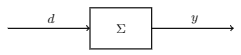
Refer to caption
Figure 1: A dynamical system
Remark 1

Definition 1 can be generalized by allowing 𝒳0\mathcal{X}_{0} to be dependent of d⁡(0)d(0). This is reasonable for systems trying to track d⁡(⋅)d(\cdot), assuming their initial tracking error is not too large. This is also reasonable for systems trying to avoid an obstacle whose position is defined by d⁡(⋅)d(\cdot), assuming the system does not start on top of the obstacle.

We wish to consider specifications on the behaviour of dynamical systems. A dynamical system can be thought of as a map from input signals d⁡(⋅)∈𝒮ndd(\cdot)\in\mathcal{S}^{n_{d}} to output signals y⁡(⋅)∈𝒮nyy(\cdot)\in\mathcal{S}^{n_{y}}, as in Fig. 1. As such, we can adopt the formulation of assume/guarantee contracts by merely making assumptions on the input variable d⁡(⋅)d(\cdot) and demanding guarantees on the output variable y⁡(⋅)y(\cdot) given the input d⁡(⋅)d(\cdot).

Definition 2

An assume/guarantee contract is a pair (𝒟,Ω)(\mathcal{D},\Omega) where 𝒟⊆𝒮nd\mathcal{D}\subseteq\mathcal{S}^{n_{d}} are the assumptions and Ω⊆𝒮nd×𝒮ny\Omega\subseteq\mathcal{S}^{n_{d}}\times\mathcal{S}^{n_{y}} are the guarantees.

In other words, we put assumptions on the input d⁡(⋅)d(\cdot) and demand guarantees on the input-output pair (d⁡(⋅),y⁡(⋅))(d(\cdot),y(\cdot)).

Example 1

We say that a system d↦yd\mapsto y has finite ℓ2\ell_{2}-gain no more than β\beta if for any d∈ℓ2d\in\ell_{2}, we have y∈ℓ2y\in\ell_{2} and ‖y‖ℓ2≤β​‖d‖ℓ2\|y\|_{\rm\ell_{2}}\leq\beta\|d\|_{\rm\ell_{2}}. This property can be written as an assume/guarantee contract 𝒞=(𝒟,Ω)\mathcal{C}=(\mathcal{D},\Omega), where 𝒟=ℓ2\mathcal{D}=\ell_{2} and Ω={(d⁡(⋅),y⁡(⋅)):‖y‖ℓ2≤β​‖d‖ℓ2}\Omega=\{(d(\cdot),y(\cdot)):\|y\|_{\rm\ell_{2}}\leq\beta\|d\|_{\rm\ell_{2}}\}.

Example 2

We say that a SISO system d↦yd\mapsto y exponentially tracks constant signals with exponent λ∈(0,1)\lambda\in(0,1) if for any constant input dd, the output yy satisfies |y⁡(k)−d⁡(k)|≤λ​|y⁡(k−1)−d⁡(k−1)||y(k)-d(k)|\leq\lambda|y(k-1)-d(k-1)| for all kk. This property can be written as an assume/guarantee contract 𝒞=(𝒟,Ω)\mathcal{C}=(\mathcal{D},\Omega), where 𝒟={d(⋅):d(k+1)=d(k),∀k}\mathcal{D}=\{d(\cdot):d(k+1)=d(k),~\forall k\} and Ω={(d(⋅),y(⋅)):|y(k+1)−d(k+1)|≤λ|y(k)−d(k)|,∀k}\Omega=\{(d(\cdot),y(\cdot)):|y(k+1)-d(k+1)|\leq\lambda|y(k)-d(k)|,~\forall k\}.

Let us now define the notion of satisfaction. This notion connects systems and assume/guarantee contracts, by defining when a given system satisfies the specifications defined by a given contract.

Definition 3

We say that a system Σ\Sigma satisfies 𝒞=(𝒟,Ω)\mathcal{C}=(\mathcal{D},\Omega) (or implements 𝒞\mathcal{C}), and write Σ⊨𝒞\Sigma\vDash\mathcal{C}, if for any d∈𝒟d\in\mathcal{D} and any y∈Σ⁡(d)y\in\Sigma(d), (d,y)∈Ω(d,y)\in\Omega.

Example 3

Consider the following contract 𝒞=(𝒟,Ω)\mathcal{C}=(\mathcal{D},\Omega): d,y∈𝒮1d,y\in\mathcal{S}^{1},

𝒟\displaystyle\mathcal{D} ={d(⋅):d(k+1)=d(k)∈[−1,1],∀k}\displaystyle=\{d(\cdot):d(k+1)=d(k)\in[-1,1],~\forall k\}
Ω\displaystyle\Omega ={(d(⋅),y(⋅)):|y(k)−d(k)|≤2−k,∀k}.\displaystyle=\{(d(\cdot),y(\cdot)):|y(k)-d(k)|\leq 2^{-k},~\forall k\}.

First, consider a system Σ1\Sigma_{1} with no state (i.e., x⁡(⋅)∈𝒮0x(\cdot)\in\mathcal{S}^{0} and 𝒳0=∅\mathcal{X}_{0}=\emptyset), A=B=C=0A=B=C=0 and D=1D=1, i.e. Σ1\Sigma_{1} is a static gain K=1K=1. Thus, for any signal d⁡(⋅)d(\cdot) we have Σ1​(d)={d}\Sigma_{1}(d)=\{d\}, implying that for any d∈𝒟d\in\mathcal{D} and y∈Σ1​(d)y\in\Sigma_{1}(d) we have (d,y)∈Ω(d,y)\in\Omega, hence Σ1⊨𝒞\Sigma_{1}\vDash\mathcal{C}. Second, consider a system Σ2\Sigma_{2} with a state x⁡(⋅)∈𝒮1x(\cdot)\in\mathcal{S}^{1} such that 𝒳0={0}\mathcal{X}_{0}=\{0\}, A=B=0.5A=B=0.5, C=1C=1 and D=0D=0. For any d⁡(⋅)∈𝒟d(\cdot)\in\mathcal{D}, there exists some v∈[−1,1]v\in[-1,1] such that d⁡(k)=v,∀kd(k)=v,~\forall k. If we feed d⁡(⋅)d(\cdot) into Σ\Sigma, we get an output y⁡(k)=x⁡(k)=(1−0.5k)​vy(k)=x(k)=(1-0.5^{k})v. Thus, |d⁡(k)−y⁡(k)|≤2−k|d(k)-y(k)|\leq 2^{-k}, as |v|≤1|v|\leq 1, and Σ2⊨𝒞\Sigma_{2}\vDash\mathcal{C}.

2.1 Refinement and Composition

One of the greatest perks of contract theory is its modularity, as one can refine a contract on a composite system by “smaller” contracts on subsystems, which can be further refined by even “smaller” contracts on individual components. The two notions supporting this idea are refinement, defining when one contract is stricter than another, and composition, defining the coupling of multiple contracts. In this subsection, we define the notion of refinement for assume/guarantee contracts, as well as a restricted notion of contract composition for cascade systems. Computational tools for these notions will be provided in the next section. We start by defining refinement:

Definition 4

Let 𝒞i=(𝒟i,Ωi)\mathcal{C}_{i}=(\mathcal{D}_{i},\Omega_{i}) be contracts for i=1,2i=1,2. We say 𝒞1\mathcal{C}_{1} refines 𝒞2\mathcal{C}_{2} (and write 𝒞1≼𝒞2\mathcal{C}_{1}\preccurlyeq\mathcal{C}_{2}) if 𝒟1⊇𝒟2\mathcal{D}_{1}\supseteq\mathcal{D}_{2} and Ω1∩(𝒟2×𝒮ny)⊆Ω2∩(𝒟2×𝒮ny)\Omega_{1}\cap(\mathcal{D}_{2}\times\mathcal{S}^{n_{y}})\subseteq\Omega_{2}\cap(\mathcal{D}_{2}\times\mathcal{S}^{n_{y}}), where nyn_{y} is the dimension of the output.

Colloquially, 𝒞1≼𝒞2\mathcal{C}_{1}\preccurlyeq\mathcal{C}_{2} if 𝒞1\mathcal{C}_{1} assumes less than 𝒞2\mathcal{C}_{2}, but guarantees more given the assumptions.

Example 4

Consider two contracts used for tracking. The first, 𝒞=(𝒟,Ω)\mathcal{C}=(\mathcal{D},\Omega) defines asymptotic tracking of certain inputs, namely d,y∈𝒮md,y\in\mathcal{S}^{m}, 𝒟⊆𝒮m\mathcal{D}\subseteq\mathcal{S}^{m}, and

Ω={(d⁡(⋅),y⁡(⋅)):limk→∞‖d⁡(k)−y⁡(k)‖=0}\displaystyle\Omega=\{(d(\cdot),y(\cdot)):\lim_{k\to\infty}\|d(k)-y(k)\|=0\}

The second, 𝒞′=(𝒟,Ω′)\mathcal{C}^{\prime}=(\mathcal{D},\Omega^{\prime}), defines exponential convergence, i.e., we take some λ∈(0,1)\lambda\in(0,1) and define:

Ω′={(d⁡(⋅),y⁡(⋅)):‖d⁡(k)−y⁡(k)‖≤λ​‖d⁡(k−1)−y⁡(k−1)‖}.\displaystyle\Omega^{\prime}=\{(d(\cdot),y(\cdot)):\|d(k)-y(k)\|\leq\lambda\|d(k-1)-y(k-1)\|\}.

By definition, we have 𝒞′≼𝒞\mathcal{C}^{\prime}\preccurlyeq\mathcal{C}.

Refinement provides a partial ordering of assume/guarantee contracts, and it is “harder” to satisfy refined contracts:

Proposition 1

Let 𝒞i=(𝒟i,Ωi)\mathcal{C}_{i}=(\mathcal{D}_{i},\Omega_{i}) be assume/guarantee contracts for i=1,2,3i=1,2,3 and Σ\Sigma be a system. Then, the following statements hold:

  • •

    𝒞1≼𝒞1\mathcal{C}_{1}\preccurlyeq\mathcal{C}_{1}.

  • •

    If 𝒞1≼𝒞2\mathcal{C}_{1}\preccurlyeq\mathcal{C}_{2} and 𝒞2≼𝒞3\mathcal{C}_{2}\preccurlyeq\mathcal{C}_{3} then 𝒞1≼𝒞3\mathcal{C}_{1}\preccurlyeq\mathcal{C}_{3}.

  • •

    If 𝒞1≼𝒞2\mathcal{C}_{1}\preccurlyeq\mathcal{C}_{2} and Σ⊨𝒞1\Sigma\vDash\mathcal{C}_{1}, then Σ⊨𝒞2\Sigma\vDash\mathcal{C}_{2}.

{pf}

We prove the claims in order. The first immediately follows from Definition 4. For the second claim, 𝒞1≼𝒞2\mathcal{C}_{1}\preccurlyeq\mathcal{C}_{2}, 𝒞2≼𝒞3\mathcal{C}_{2}\preccurlyeq\mathcal{C}_{3} imply that 𝒟1⊇𝒟2⊇𝒟3\mathcal{D}_{1}\supseteq\mathcal{D}_{2}\supseteq\mathcal{D}_{3}, and that:

Ω1∩(𝒟2×𝒮ny)⊆Ω2∩(𝒟2×𝒮ny)\displaystyle\Omega_{1}\cap(\mathcal{D}_{2}\times\mathcal{S}^{n_{y}})\subseteq\Omega_{2}\cap(\mathcal{D}_{2}\times\mathcal{S}^{n_{y}})
Ω2∩(𝒟3×𝒮ny)⊆Ω3∩(𝒟3×𝒮ny)\displaystyle\Omega_{2}\cap(\mathcal{D}_{3}\times\mathcal{S}^{n_{y}})\subseteq\Omega_{3}\cap(\mathcal{D}_{3}\times\mathcal{S}^{n_{y}})

by intersecting both sides of the first equation with (𝒟3×𝒮ny)(\mathcal{D}_{3}\times\mathcal{S}^{n_{y}}), and using 𝒟3⊆𝒟2\mathcal{D}_{3}\subseteq\mathcal{D}_{2}, we conclude that Ω1∩(𝒟3×𝒮ny)⊆Ω3∩(𝒟3×𝒮ny)\Omega_{1}\cap(\mathcal{D}_{3}\times\mathcal{S}^{n_{y}})\subseteq\Omega_{3}\cap(\mathcal{D}_{3}\times\mathcal{S}^{n_{y}}), hence 𝒞1≼𝒞3\mathcal{C}_{1}\preccurlyeq\mathcal{C}_{3}. Lastly, suppose Σ⊨𝒞1\Sigma\vDash\mathcal{C}_{1} and 𝒞1≼𝒞2\mathcal{C}_{1}\preccurlyeq\mathcal{C}_{2}, and we show that Σ⊨𝒞2\Sigma\vDash\mathcal{C}_{2}. Take any d∈𝒟2d\in\mathcal{D}_{2} and y∈Σ⁡(d)y\in\Sigma(d). As 𝒞1≼𝒞2\mathcal{C}_{1}\preccurlyeq\mathcal{C}_{2}, we conclude that d∈𝒟1d\in\mathcal{D}_{1}, so Σ⊨𝒞1\Sigma\vDash\mathcal{C}_{1} implies that (d,y)∈Ω1(d,y)\in\Omega_{1}. Noting that d∈𝒟2d\in\mathcal{D}_{2} and 𝒞1≼𝒞2\mathcal{C}_{1}\preccurlyeq\mathcal{C}_{2}, we conclude that (d,y)∈Ω2(d,y)\in\Omega_{2}. □\Box Proposition 1 is important in contract theory, as it shows two key properties. First, if we have an original contract 𝒞\mathcal{C} and a refined contract 𝒞′\mathcal{C}^{\prime}, any system satisfying 𝒞′\mathcal{C}^{\prime} also satisfies 𝒞\mathcal{C}. Second, if we have an original contract 𝒞\mathcal{C} and a refined contract 𝒞′\mathcal{C}^{\prime}, any refinement of 𝒞′\mathcal{C}^{\prime} is also a refinement of 𝒞\mathcal{C}. These properties allow us to refine a contract on a composite system by multiple contracts on the individual subsystems, which can be further refined by a plethora of contracts on the individual components in the system. If each component satisfies its corresponding contract, then the composite system will satisfy the original contract.

We now move to cascaded composition. Consider the block diagram in Fig. 2.

Refer to caption
Figure 2: Cascade of contracts

Define the cascaded composition of 𝒞1\mathcal{C}_{1} and 𝒞2\mathcal{C}_{2} such that if Σ1⊨𝒞1\Sigma_{1}\vDash\mathcal{C}_{1} and Σ2⊨𝒞2\Sigma_{2}\vDash\mathcal{C}_{2}, the cascade of Σ1\Sigma_{1} and Σ2\Sigma_{2} satisfies the composition 𝒞1⊗𝒞2\mathcal{C}_{1}\otimes\mathcal{C}_{2}. First, let us define the cascade of systems:

Definition 2.1

Let Σi=(𝒳i,Ai,Bi,Ci,Di)\Sigma_{i}=(\mathcal{X}_{i},A_{i},B_{i},C_{i},D_{i}) be systems for i=1,2i=1,2. The cascade Σ1⊗Σ2=(𝒳⊗,A⊗,B⊗,C⊗,D⊗)\Sigma_{1}\otimes\Sigma_{2}=(\mathcal{X}_{\otimes},A_{\otimes},B_{\otimes},C_{\otimes},D_{\otimes}) has input d⊗=d1d_{\otimes}=d_{1}, output y⊗=y2y_{\otimes}=y_{2}, state x⊗=[x1⊤,x2⊤]⊤x_{\otimes}=[x_{1}^{\top},x_{2}^{\top}]^{\top}, allowable initial states 𝒳⊗=𝒳1×𝒳2\mathcal{X}_{\otimes}=\mathcal{X}_{1}\times\mathcal{X}_{2}, and matrices A⊗=[A10B2​C1A2]A_{\otimes}=\left[\begin{smallmatrix}A_{1}&0\\ B_{2}C_{1}&A_{2}\end{smallmatrix}\right], B⊗=[B1B2​D1]B_{\otimes}=\left[\begin{smallmatrix}B_{1}\\ B_{2}D_{1}\end{smallmatrix}\right], C⊗=[D2​C1C2],C_{\otimes}=\left[\begin{smallmatrix}D_{2}C_{1}&C_{2}\end{smallmatrix}\right], D⊗=D2​D1D_{\otimes}=D_{2}D_{1}.

Consider two contracts 𝒞i=(𝒟i,Ωi)\mathcal{C}_{i}=(\mathcal{D}_{i},\Omega_{i}) as in Fig. 2. When defining a contract that is satisfied by the composition, we at least need d1∈𝒟1d_{1}\in\mathcal{D}_{1} and (d2,y2)∈Ω2(d_{2},y_{2})\in\Omega_{2}. The latter also requires d2∈𝒟2d_{2}\in\mathcal{D}_{2}, while the former only implies (d1,y1)∈Ω1(d_{1},y_{1})\in\Omega_{1}. This motivates the following definition:

Definition 2.2

For two contracts 𝒞i=(𝒟i,Ωi)\mathcal{C}_{i}=(\mathcal{D}_{i},\Omega_{i}), the cascaded composition is 𝒞1⊗𝒞2=(𝒟⊗,Ω⊗)\mathcal{C}_{1}\otimes\mathcal{C}_{2}=(\mathcal{D}_{\otimes},\Omega_{\otimes}) with input d⊗=d1d_{\otimes}=d_{1}, output y⊗=y2y_{\otimes}=y_{2},

𝒟⊗\displaystyle\mathcal{D}_{\otimes} ={d⊗:d⊗∈𝒟1,((d⊗,y1)∈Ω1⟹y1∈𝒟2)},\displaystyle=\{d_{\otimes}:~d_{\otimes}\in\mathcal{D}_{1},\left((d_{\otimes},y_{1})\in\Omega_{1}\implies y_{1}\in\mathcal{D}_{2}\right)\},
Ω⊗\displaystyle\Omega_{\otimes} ={(d⊗,y⊗):∃d2=y1,(d⊗,y1)∈Ω1,(d2,y⊗)∈Ω2}.\displaystyle=\{(d_{\otimes},y_{\otimes}):\exists d_{2}=y_{1},(d_{\otimes},y_{1})\in\Omega_{1},(d_{2},y_{\otimes})\in\Omega_{2}\}.

We now prove our main claim about contract composition:

Proposition 2

Let 𝒞1,𝒞2\mathcal{C}_{1},\mathcal{C}_{2} and Σ1,Σ2\Sigma_{1},\Sigma_{2} be contracts and systems with inputs d1,d2d_{1},d_{2} and outputs y1,y2y_{1},y_{2}. If Σ1⊨𝒞1\Sigma_{1}\vDash\mathcal{C}_{1} and Σ2⊨𝒞2\Sigma_{2}\vDash\mathcal{C}_{2}, then Σ1⊗Σ2⊨𝒞1⊗𝒞2\Sigma_{1}\otimes\Sigma_{2}\vDash\mathcal{C}_{1}\otimes\mathcal{C}_{2}.

{pf}

Denote 𝒞i=(𝒟i,Ωi)\mathcal{C}_{i}=(\mathcal{D}_{i},\Omega_{i}). By Definition 2.1, for any d⊗=d1d_{\otimes}=d_{1} and y⊗=y2y_{\otimes}=y_{2}, y⊗∈Σ1⊗Σ2​(d⊗)y_{\otimes}\in\Sigma_{1}\otimes\Sigma_{2}(d_{\otimes}) if and only if there exists some d2=y1∈Σ1​(d⊗)d_{2}=y_{1}\in\Sigma_{1}(d_{\otimes}) such that y⊗∈Σ2​(d2)y_{\otimes}\in\Sigma_{2}(d_{2}). Now, suppose d⊗=d1∈𝒟⊗d_{\otimes}=d_{1}\in\mathcal{D}_{\otimes} and y⊗=y2∈Σ1⊗Σ2​(d⊗)y_{\otimes}=y_{2}\in\Sigma_{1}\otimes\Sigma_{2}(d_{\otimes}), and let d2=y1d_{2}=y_{1} be such that d2=y1∈Σ1​(d⊗)d_{2}=y_{1}\in\Sigma_{1}(d_{\otimes}) such that y⊗∈Σ2​(d2)y_{\otimes}\in\Sigma_{2}(d_{2}). As d1∈𝒟1,y1∈Σ1​(d1)d_{1}\in\mathcal{D}_{1},y_{1}\in\Sigma_{1}(d_{1}) and Σ1⊨𝒞1\Sigma_{1}\vDash\mathcal{C}_{1}, we conclude that (d1,y1)∈Ω1(d_{1},y_{1})\in\Omega_{1}. As d⊗∈𝒟⊗d_{\otimes}\in\mathcal{D}_{\otimes}, we get d2∈𝒟2d_{2}\in\mathcal{D}_{2}. Adding y2∈Σ2​(d2)y_{2}\in\Sigma_{2}(d_{2}) and Σ2⊨𝒞2\Sigma_{2}\vDash\mathcal{C}_{2} gives that (d2,y2)∈Ω2(d_{2},y_{2})\in\Omega_{2}, hence (d⊗,y⊗)∈Ω⊗(d_{\otimes},y_{\otimes})\in\Omega_{\otimes}. Thus Σ1⊗Σ2⊨𝒞1⊗𝒞2\Sigma_{1}\otimes\Sigma_{2}\vDash\mathcal{C}_{1}\otimes\mathcal{C}_{2}. □\Box

3 Computational Tools for Verification

The previous section presented abstract assume/guarantee contracts for discrete-time dynamical systems, as well the notions of satisfaction, refinement and cascaded composition. In this section, we present computational tools for verifying satisfaction and refinement, relying on mathematical induction and linear programming. We rely on linearity of both the systems and specifications. More precisely, we present computational tools for assumptions of the form A1​d​(k+1)+A0​d​(k)≤a0A^{1}d(k+1)+A^{0}d(k)\leq a^{0} for all kk, and guarantees of the form G1​[d⁡(k+1)y⁡(k+1)]+G0​[d⁡(k)y⁡(k)]≤g0G^{1}\left[\begin{smallmatrix}d(k+1)\\ y(k+1)\end{smallmatrix}\right]+G^{0}\left[\begin{smallmatrix}d(k)\\ y(k)\end{smallmatrix}\right]\leq g^{0} for all kk, where A0,A1,G0,G1A^{0},A^{1},G^{0},G^{1} are matrices and a0,g0a^{0},g^{0} are vectors of appropriate dimensions. Specifications of this form include general bounded signals, as well as outputs of dynamical systems (e.g., the input dd is the output of a given first-order system). In Section 4, we use specifications of this form to model a contract where the input is assumed to be a (constrained) trajectory of a dynamical system, and the guarantee is a linear inequality defining safe behaviour.

3.1 Verifying Satisfaction

Consider a contract 𝒞=(𝒟,Ω)\mathcal{C}=(\mathcal{D},\Omega) where

𝒟\displaystyle\mathcal{D} ={d(⋅):A1d(k+1)+A0d(k)≤a0,∀k},\displaystyle=\{d(\cdot):A^{1}d(k+1)+A^{0}d(k)\leq a^{0},~\forall k\}, (2)
Ω\displaystyle\Omega ={(d(⋅),y(⋅)):G1[d⁡(k+1)y⁡(k+1)]+G0[d⁡(k)y⁡(k)]≤g0,∀k}\displaystyle=\left\{(d(\cdot),y(\cdot)):G^{1}\left[\begin{smallmatrix}d(k+1)\\ y(k+1)\end{smallmatrix}\right]+G^{0}\left[\begin{smallmatrix}d(k)\\ y(k)\end{smallmatrix}\right]\leq g^{0},~\forall k\right\} (3)

for given A0,A1,G0,G1,a0,g0A^{0},A^{1},G^{0},G^{1},a^{0},g^{0}.

Example 5

Suppose d⁡(⋅)∈𝒮2d(\cdot)\in\mathcal{S}^{2} is the position of a robot in a field, parameterized by ℱ={p∈ℝ2:L1≤p1≤U1,L2≤p2≤U2}\mathcal{F}=\{p\in\mathbb{R}^{2}:L_{1}\leq p_{1}\leq U_{1},L_{2}\leq p_{2}\leq U_{2}\} for constants L1,L2,U1,U2L_{1},L_{2},U_{1},U_{2}. Assume that for all k∈ℕk\in\mathbb{N}, d⁡(k)∈ℱd(k)\in\mathcal{F} and d⁡(k+1)=d⁡(k)+v⁡(k)d(k+1)=d(k)+v(k) for some velocity v⁡(k)v(k) bounded by VmaxV_{\rm max}, i.e. that −[Vmax,Vmax]⊤≤d⁡(k+1)−d⁡(k)≤[Vmax,Vmax]⊤-[V_{\rm max},V_{\rm max}]^{\top}\leq d(k+1)-d(k)\leq[V_{\rm max},V_{\rm max}]^{\top}. The assumptions are of the form (2) where:

A0=[1−1001−100001−1001−1]⊤,A1=[0000−11000000001−1]⊤\displaystyle A^{0}=\left[\begin{smallmatrix}1&-1&0&0&1&-1&0&0\\ 0&0&1&-1&0&0&1&-1\end{smallmatrix}\right]^{\top},~A^{1}=\left[\begin{smallmatrix}0&0&0&0&-1&1&0&0\\ 0&0&0&0&0&0&1&-1\end{smallmatrix}\right]^{\top}

and a0=[U1L1U2L2−VmaxVmax−VmaxVmax]⊤a^{0}=\left[\begin{smallmatrix}U_{1}&L_{1}&U_{2}&L_{2}&-V_{\rm max}&V_{\rm max}&-V_{\rm max}&V_{\rm max}\end{smallmatrix}\right]^{\top}.

Let us make the following assumption on (2),(3):

Definition 3.1

Given two matrices V1,V0V^{1},V^{0} and a vector v0v^{0}, we say (V1,V0,v0)(V^{1},V^{0},v^{0}) is extendable if for any two vectors u0,u1u_{0},u_{1} and V1​u1+V0​u0≤v0V^{1}u_{1}+V^{0}u_{0}\leq v^{0}, there exists some vector u2u_{2} such that V1​u2+V0​u1≤v0V^{1}u_{2}+V^{0}u_{1}\leq v^{0}.

Assuming (A1,A0,a0)(A^{1},A^{0},a^{0}) (or (G1,G0,g0)(G^{1},G^{0},g^{0})) is extendable is not very restrictive. It is equivalent to assuming that any signal v⁡(⋅)v(\cdot) adhering to the assumption, and defined for times k=0,…,nk=0,\ldots,n, can be extended to a signal defined for all times k∈ℕk\in\mathbb{N} while satisfying the assumption.

Theorem 3

Let 𝒞=(𝒟,Ω)\mathcal{C}=(\mathcal{D},\Omega) be a contract with (2) and (3), and let Σ=(𝒳0,A,B,C,D)\Sigma=(\mathcal{X}_{0},A,B,C,D) be a system with x∈𝒮nx\in\mathcal{S}^{n}. Assume that (A1,A0,a0)(A^{1},A^{0},a^{0}) is extendable. Then Σ⊨𝒞\Sigma\vDash\mathcal{C} if and only if for any n∈ℕn\in\mathbb{N}, the following condition holds: for any d0,d1,…,dn+1,x0,x1,…,xn+1,y0,y1,…,yn+1d_{0},d_{1},\ldots,d_{n+1},x_{0},x_{1},\ldots,x_{n+1},y_{0},y_{1},\ldots,y_{n+1}, the condition:

{x0∈𝒳0,G1​[dk+1yk+1]+G0​[dkyk]≤g0,∀k=0,…,n−1,A1​dk+1+A0​dk≤a0,∀k=0,…,n,xk+1=A​xk+B​dk,∀k=0,…,n,yk=C​xk+D​dk,∀k=0,…,n+1,\displaystyle\begin{cases}x_{0}\in\mathcal{X}_{0},\\ G^{1}\left[\begin{smallmatrix}d_{k+1}\\ y_{k+1}\end{smallmatrix}\right]+G^{0}\left[\begin{smallmatrix}d_{k}\\ y_{k}\end{smallmatrix}\right]\leq g^{0},&\forall k=0,\ldots,n-1,\\ A^{1}d_{k+1}+A^{0}d_{k}\leq a^{0},&\forall k=0,\ldots,n,\\ x_{k+1}=Ax_{k}+Bd_{k},&\forall k=0,\ldots,n,\\ y_{k}=Cx_{k}+Dd_{k},&\forall k=0,\ldots,n+1,\end{cases} (4)

implies G1​[dn+1yn+1]+G0​[dnyn]≤g0G^{1}\left[\begin{smallmatrix}d_{n+1}\\ y_{n+1}\end{smallmatrix}\right]+G^{0}\left[\begin{smallmatrix}d_{n}\\ y_{n}\end{smallmatrix}\right]\leq g^{0}.

{pf}

Suppose first that whenever (4) holds we have G1​[dn+1yn+1]+G0​[dnyn]≤g0G^{1}\left[\begin{smallmatrix}d_{n+1}\\ y_{n+1}\end{smallmatrix}\right]+G^{0}\left[\begin{smallmatrix}d_{n}\\ y_{n}\end{smallmatrix}\right]\leq g^{0}, and take any d∈𝒟d\in\mathcal{D} and y∈Σ⁡(d)y\in\Sigma(d). Note that A1​d​(k+1)+A0​d​(k)≤a0A^{1}d(k+1)+A^{0}d(k)\leq a^{0} holds for all kk, and for some signal x⁡(⋅)x(\cdot), both x⁡(k+1)=A​x​(k)+B​d​(k)x(k+1)=Ax(k)+Bd(k) and y⁡(k)=C​x​(k)+D​d​(k)y(k)=Cx(k)+Dd(k) hold for all kk, as well as x⁡(0)∈𝒳0x(0)\in\mathcal{X}_{0}. Choosing dk=d⁡(k),xk=x⁡(k)d_{k}=d(k),x_{k}=x(k) and yk=y⁡(k)y_{k}=y(k) for all k=0,…,n+1k=0,\ldots,n+1, and using the implication (4), we conclude that G1​[d⁡(k+1)y⁡(k+1)]+G0​[d⁡(k)y⁡(k)]≤g0G^{1}\left[\begin{smallmatrix}d(k+1)\\ y(k+1)\end{smallmatrix}\right]+G^{0}\left[\begin{smallmatrix}d(k)\\ y(k)\end{smallmatrix}\right]\leq g^{0} can be proved for all k∈ℕk\in\mathbb{N} by induction on the value of kk, i.e., Σ⊨𝒞\Sigma\vDash\mathcal{C}.

Conversely, suppose Σ⊨𝒞\Sigma\vDash\mathcal{C}, and take n∈ℕn\in\mathbb{N} and some d0,x0,y0,…,dn+1,xn+1,yn+1d_{0},x_{0},y_{0},\ldots,d_{n+1},x_{n+1},y_{n+1} such that (4) holds, and we show that G1​[dn+1yn+1]+G0​[dnyn]≤g0G^{1}\left[\begin{smallmatrix}d_{n+1}\\ y_{n+1}\end{smallmatrix}\right]+G^{0}\left[\begin{smallmatrix}d_{n}\\ y_{n}\end{smallmatrix}\right]\leq g^{0}. We show that there exist signals d^​(⋅),y^​(⋅)\hat{d}(\cdot),\hat{y}(\cdot) such that y^∈Σ⁡(d^)\hat{y}\in\Sigma(\hat{d}), d^∈𝒟\hat{d}\in\mathcal{D}, and d^​(k)=dk,y^​(k)=yk\hat{d}(k)=d_{k},\hat{y}(k)=y_{k} hold for k=0,1,…,n+1k=0,1,\ldots,n+1. If we show that, we can use Σ⊨𝒞\Sigma\vDash\mathcal{C} to conclude (d^,y^)∈Ω(\hat{d},\hat{y})\in\Omega, implying the desired inequality at time k=n+1k=n+1. Thus, we prove that the signals d^​(⋅),y^​(⋅)\hat{d}(\cdot),\hat{y}(\cdot) defined above exist.

By extendibility, there exists a signal d^∈𝒟\hat{d}\in\mathcal{D} such that d^​(k)=dk\hat{d}(k)=d_{k} for k=0,…,n+1k=0,\ldots,n+1. Choose x^​(0)=x0\hat{x}(0)=x_{0} and define x^​(k+1)=A​x^​(k)+B​d^​(k)\hat{x}(k+1)=A\hat{x}(k)+B\hat{d}(k), y^​(k)=C​x^​(k)+D​d^​(k)\hat{y}(k)=C\hat{x}(k)+D\hat{d}(k) for any time k∈ℕk\in\mathbb{N}. On one hand, x^​(k)=xk\hat{x}(k)=x_{k} and y^​(k)=yk\hat{y}(k)=y_{k} hold for all k=0,…,n+1k=0,\ldots,n+1. On the other hand, y^∈Σ⁡(d^)\hat{y}\in\Sigma(\hat{d}). We thus showed the existence of d^​(⋅),y^​(⋅)\hat{d}(\cdot),\hat{y}(\cdot), which implies that the desired implication holds. ■\hfill\blacksquare

The previous theorem allows one to verify that a given system satisfies a given contract by proving a sequence of (infinitely many) implications of the form (4). Roughly speaking, this implication guarantees that if the system implements the contract up to time nn, then it implements the contract up to time n+1n+1. Even though this formulation requires infinitely many steps in general, we will soon see that only finitely many implications of the form (4) needs to be verified. Importantly, the implication (4) can be cast as an optimization problem. For any n,p∈ℕn,p\in\mathbb{N} such that n≥pn\geq p, we consider the following optimization problem:

max\displaystyle\max~ maxi⁡[ei⊤​(G1​[dn+1yn+1]+G0​[dnyn]−g0)]\displaystyle~\max_{i}~\left[{\rm e}_{i}^{\top}\left(G^{1}\left[\begin{smallmatrix}d_{n+1}\\ y_{n+1}\end{smallmatrix}\right]+G^{0}\left[\begin{smallmatrix}d_{n}\\ y_{n}\end{smallmatrix}\right]-g^{0}\right)\right] (5)
s.t.\displaystyle{\rm s.t.}~ G1​[dk+1yk+1]+G0​[dkyk]≤g0,∀k=p,…,n−1,\displaystyle~G^{1}\left[\begin{smallmatrix}d_{k+1}\\ y_{k+1}\end{smallmatrix}\right]+G^{0}\left[\begin{smallmatrix}d_{k}\\ y_{k}\end{smallmatrix}\right]\leq g^{0}~~~~,\forall k=p,\ldots,n-1,
A1​dk+1+A0​dk≤a0,∀k=p,…,n,\displaystyle~A^{1}d_{k+1}+A^{0}d_{k}\leq a^{0}~~~~~~~~~~~~,\forall k=p,\ldots,n,
xk+1=A​xk+B​dk,∀k=p,…,n,\displaystyle~x_{k+1}=Ax_{k}+Bd_{k}~~~~~~~~~~~~~~,\forall k=p,\ldots,n,
yk=C​xk+D​dk,∀k=p,…,n+1,\displaystyle~y_{k}=Cx_{k}+Dd_{k}~~~~~~~~~~~~~~~~~,\forall k=p,\ldots,n+1,
xp∈𝒳p,\displaystyle~x_{p}\in\mathcal{X}_{p},
dk∈ℝnd,xk∈ℝnx,yk∈ℝny,∀k=p,…,n+1,\displaystyle~d_{k}\in\mathbb{R}^{n_{d}},x_{k}\in\mathbb{R}^{n_{x}},y_{k}\in\mathbb{R}^{n_{y}},\forall k=p,\ldots,n+1,

where ei\rm e_{i} are the standard basis elements, and 𝒳p\mathcal{X}_{p} for p=1,2,…,np=1,2,\ldots,n are sets to be defined later. We denote this problem as Vn,n−pV_{n,n-p} and let θn,n−p\theta_{n,n-p} be its value. Here, nn is the last time at which the we know the guarantee holds, pp is the first time we consider, and ℓ=n−p\ell=n-p is the length of history we consider. When taking p=0p=0, the problem (5) computes the “worst-case violation” of the guarantee at time n+1n+1, given that the guarantees hold up to time nn. For that reason, Theorem 3 can be restated as:

Corollary 4

Under the assumptions of Theorem 3, Σ⊨𝒞\Sigma\vDash\mathcal{C} if and only if θn,n≤0\theta_{n,n}\leq 0 for all n∈ℕn\in\mathbb{N}.

{pf}

θn,n≤0\theta_{n,n}\leq 0 if and only if whenever (4) holds, G1​[dn+1yn+1]+G0​[dnyn]−g0≤0G^{1}\left[\begin{smallmatrix}d_{n+1}\\ y_{n+1}\end{smallmatrix}\right]+G^{0}\left[\begin{smallmatrix}d_{n}\\ y_{n}\end{smallmatrix}\right]-g^{0}\leq 0 also holds, which is equivalent to Σ⊨𝒞\Sigma\vDash\mathcal{C} by Theorem 3. □\Box

The corollary implies that it suffices to compute θn,n\theta_{n,n} for all n∈ℕn\in\mathbb{N} in order to verify Σ⊨𝒞\Sigma\vDash\mathcal{C}. We however prefer to compute θn,ℓ\theta_{n,\ell} for small ℓ=n−p\ell=n-p, as this leads to a simpler problem that can be solved more efficiently with existing numerical methods. The main difficulty in reducing the verification to problems Vn,ℓV_{n,\ell} for small ℓ\ell is that it requires knowledge of the state trajectory x⁡(⋅)x(\cdot) at time p=n−lp=n-l, captured in (5) via the constraint xp∈𝒳px_{p}\in\mathcal{X}_{p}. This simply reduces to the initial value x0∈𝒳0x_{0}\in\mathcal{X}_{0} for problems Vn,nV_{n,n}.

An efficient solution of Vn,ℓV_{n,\ell} for small ℓ\ell requires a characterization of 𝒳p\mathcal{X}_{p} satisfying the following criteria. First, it is desirable that 𝒳p\mathcal{X}_{p} is a polyhedral set11 1 i.e., it is of the form {x:F​x≤f}\{x:Fx\leq f\} for a matrix FF and a vector ff., as (5) reduces to a linear problem for which efficient solvers are available, e.g., Yalmip (Löfberg 2004). Second, we would like 𝒳p\mathcal{X}_{p} to be independent of pp, as this will imply verification of contract satisfaction can be done by solving a finite number of optimization problems (thus not requiring the computation of all θn,n\theta_{n,n} as in Corollary 4). Third, Vn,ℓV_{n,\ell} is equivalent to Vn+1,ℓV_{n+1,\ell} where 𝒳p+1\mathcal{X}_{p+1} is the image of 𝒳p\mathcal{X}_{p} under the dynamics xp+1=A​xp+B​dpx_{p+1}=Ax_{p}+Bd_{p}. Combining the last two points, we search for 𝒳p\mathcal{X}_{p} which is a robust invariant set.

However, these criteria might be contradictory. The last two dictate choosing 𝒳p\mathcal{X}_{p} as smallest robust invariant set containing 𝒳0\mathcal{X}_{0}, but this set might not be polyhedral even if 𝒳0={0}\mathcal{X}_{0}=\{0\} (Fisher and Gayek 1988). In fact, the question of whether the minimal robust invariant set containing 𝒳0={0}\mathcal{X}_{0}=\{0\} is polyhedral is related to the rationality of the eigenvalues of the matrix AA of Σ\Sigma. We can try and find some polyhedral robust invariant set containing 𝒳0\mathcal{X}_{0}, not necessarily the smallest one. Rakovic et al. 2005 offer a very partial solution for 𝒳0={0}\mathcal{X}_{0}=\{0\}, but a general solution is not known to the authors.

To avoid these difficulties, we simply set 𝒳p=ℝnx\mathcal{X}_{p}=\mathbb{R}^{n_{x}}, at the cost of a more conservative test for contract implementation. Namely, a choice of 𝒳p\mathcal{X}_{p} that is larger than necessary (i.e., larger than the smallest robust invariant set containing 𝒳0\mathcal{X}_{0}) will make the demand θn,ℓ≤0\theta_{n,\ell}\leq 0 stricter. The following theorem formalizes this case.

Theorem 5

Let Σ=(𝒳0,A,B,C,D)\Sigma=(\mathcal{X}_{0},A,B,C,D) be a system, and let ν\nu be its observability index. Take a contract 𝒞=(𝒟,Ω)\mathcal{C}=(\mathcal{D},\Omega) such that (2) and (3) hold. Define 𝒳p=ℝnx\mathcal{X}_{p}=\mathbb{R}^{n_{x}} for all p≠0p\neq 0. The following claims hold:

  • •

    For any n∈ℕ,θn,n≤θn,n−1≤θn,n−2≤…≤θn,0n\in\mathbb{N},\theta_{n,n}\leq\theta_{n,n-1}\leq\theta_{n,n-2}\leq\ldots\leq\theta_{n,0}. Moreover, for any ℓ≥0\ell\geq 0, we have θℓ,ℓ≤θℓ+1,ℓ=θℓ+2,ℓ=θℓ+3,ℓ=⋯\theta_{\ell,\ell}\leq\theta_{\ell+1,\ell}=\theta_{\ell+2,\ell}=\theta_{\ell+3,\ell}=\cdots.

  • •

    Suppose 𝒟⋆={(d0,d1):A1​d1+A0​d0≤a0}\mathcal{D}_{\star}=\{(d_{0},d_{1}):A^{1}d_{1}+A^{0}d_{0}\leq a^{0}\} is bounded, and that for any bounded set E⊆ℝ2​ndE\subseteq\mathbb{R}^{2n_{d}}, the intersection of E×ℝ2​nyE\times\mathbb{R}^{2n_{y}} with Ω⋆={(d0,d1,y0,y1):G1​[d1y1]+G0​[d0y0]≤g0}\Omega_{\star}=\{(d_{0},d_{1},y_{0},y_{1}):G^{1}\left[\begin{smallmatrix}d_{1}\\ y_{1}\end{smallmatrix}\right]+G^{0}\left[\begin{smallmatrix}d_{0}\\ y_{0}\end{smallmatrix}\right]\leq g^{0}\} is bounded. Then θn,ℓ<∞\theta_{n,\ell}<\infty for n≥ℓ≥ν−1n\geq\ell\geq\nu-1, and θn,ℓ=∞\theta_{n,\ell}=\infty if n,ν−1>ℓn,\nu-1>\ell.

  • •

    Given ℓ≥0\ell\geq 0, if θn,n≤0\theta_{n,n}\leq 0 for any 0≤n<ℓ0\leq n<\ell and θℓ+1,ℓ≤0\theta_{\ell+1,\ell}\leq 0, then Σ⊨𝒞\Sigma\vDash\mathcal{C}.

{pf}

We prove the claims in order. First, choose any 0≤p≤n−10\leq p\leq n-1. The problem Vn,n−pV_{n,n-p} is achieved from Vn,n−p+1V_{n,n-p+1} by changing two constraints. First, we remove the constraints that the guarantees, assumptions and dynamics hold at time p−1p-1. Second, while the problem Vn,n−pV_{n,n-p} restricts xp∈ℝnx_{p}\in\mathbb{R}^{n}, Vn,n−p+1V_{n,n-p+1} restricts xpx_{p} to be achieved from the dynamics (via xp−1∈ℝnx_{p-1}\in\mathbb{R}^{n} and xp=A​xp−1+B​dp−1x_{p}=Ax_{p-1}+Bd_{p-1}). Thus, Vn,n−p+1V_{n,n-p+1} has the same cost function as Vn,n−pV_{n,n-p}, but stricter constraints. In particular, as both problems are maximization problems, we conclude θn,n−p+1≤θn−p\theta_{n,n-p+1}\leq\theta_{n-p}, as desired. Similarly, Vn+1,ℓV_{n+1,\ell} is achieved from Vn,ℓV_{n,\ell} by changing the names dk,xk,ykd_{k},x_{k},y_{k} to dk+1,xk+1,yk+1d_{k+1},x_{k+1},y_{k+1}, and changing the set of initial conditions from 𝒳0\mathcal{X}_{0} to ℝnx\mathbb{R}^{n_{x}} (only if n=ℓn=\ell). We can therefore similarly derive θn,n≤θn+1,n=θn+2,n=θn+3,n=⋯\theta_{n,n}\leq\theta_{n+1,n}=\theta_{n+2,n}=\theta_{n+3,n}=\cdots.

We move to the second claim. By the first part, it suffices to show that θn,ν−1<∞\theta_{n,\nu-1}<\infty. Consider a feasible solution dn−ν+1,xn−ν+1,yn−ν+1,…,dn+1,xn+1,yn+1d_{n-\nu+1},x_{n-\nu+1},y_{n-\nu+1},\ldots,d_{n+1},x_{n+1},y_{n+1} to Vn,ν−1V_{n,\nu-1}. On one hand, as 𝒟⋆\mathcal{D}_{\star} is bounded, (𝒟⋆×ℝ2​ny)∩Ω⋆(\mathcal{D}_{\star}\times\mathbb{R}^{2n_{y}})\cap\Omega_{\star} is bounded, meaning that for some constant M0>0M_{0}>0, we have ‖dk‖,‖yk‖,‖dn+1‖≤M0\|d_{k}\|,\|y_{k}\|,\|d_{n+1}\|\leq M_{0} for k=n−ν+1,…,nk=n-\nu+1,\ldots,n. On the other hand, p𝒪​(xn−ν+1)p_{\mathcal{O}}(x_{n-\nu+1}) can be achieved as a linear combination of yn−ν+1,…,yny_{n-\nu+1},\ldots,y_{n} and dn−ν+1,…,dnd_{n-\nu+1},\ldots,d_{n} using 𝒪ν\mathcal{O}_{\nu}. Combining the two, we find a constant M1>0M_{1}>0 depending on M0M_{0} and 𝒪ν\mathcal{O}_{\nu} such that ‖p𝒪​(xn−ν+1)‖≤M1\|p_{\mathcal{O}}(x_{n-\nu+1})\|\leq M_{1}. As ‖dk‖≤M0\|d_{k}\|\leq M_{0} for all kk, we get that ‖p𝒪​(xn−ν+k)‖≤Mk\|p_{\mathcal{O}}(x_{n-\nu+k})\|\leq M_{k} for k=1,2,…,ν+1k=1,2,\ldots,\nu+1, where Mk=‖A‖​Mk−1+‖B‖​M0M_{k}=\|A\|M_{k-1}+\|B\|M_{0}, hence ‖yn+1‖≤‖C‖​Mν+1+‖D‖​M0\|y_{n+1}\|\leq\|C\|M_{\nu+1}+\|D\|M_{0}. Thus, the set of feasible {dk,yk}k\{d_{k},y_{k}\}_{k} for Vn,ν−1V_{n,\nu-1} is bounded, and θn,ν−1<∞\theta_{n,\nu-1}<\infty. One can similarly show that θn,ℓ=∞\theta_{n,\ell}=\infty for ℓ≤ν−2\ell\leq\nu-2.

We now consider the third claim. By Corollary 4, it suffices to show θn,n≤0\theta_{n,n}\leq 0 for all n≥ℓn\geq\ell. We prove these inequalities using part 1 of this theorem. First, for n≥ℓ+1n\geq\ell+1, we have θn,n≤θn,ℓ≤θℓ+1,ℓ≤0\theta_{n,n}\leq\theta_{n,\ell}\leq\theta_{\ell+1,\ell}\leq 0. Second, for n=ℓn=\ell, we have θn,n=θℓ,ℓ≤θℓ+1,ℓ≤0\theta_{n,n}=\theta_{\ell,\ell}\leq\theta_{\ell+1,\ell}\leq 0. ■\hfill\blacksquare

Remark 3.2

Theorem 5 shows that θℓ+1,ℓ=∞\theta_{\ell+1,\ell}=\infty if ℓ≤ν−2\ell\leq\nu-2. Thus, we will use the third part of Theorem 5 for ℓ=ν−1\ell=\nu-1 to verify implementation.

Remark 3.3

Consider Vn,pV_{n,p} for 𝒳p=ℝnx\mathcal{X}_{p}=\mathbb{R}^{n_{x}}. By using the transfer function associated with the state-space system (A,B,C,D)(A,B,C,D), we can find matrices E1,…,EmE_{1},\ldots,E_{m} and F0,…,FmF_{0},\ldots,F_{m} such that the state-space representation is equivalent to the recursive equation y⁡(k)=∑r=1mEr​y​(k−r)+∑r=0mFr​d​(k−r)y(k)=\sum_{r=1}^{m}E_{r}y(k-r)+\sum_{r=0}^{m}F_{r}d(k-r). Thus, Vn,ℓV_{n,\ell} for ℓ≥m\ell\geq m, p=n−ℓp=n-\ell and 𝒳p=ℝnx\mathcal{X}_{p}=\mathbb{R}^{n_{x}} can be recast as:

max\displaystyle\max~ maxi⁡[ei⊤​(G1​[dn+1yn+1]+G0​[dnyn]−g0)]\displaystyle~\max_{i}\left[{\rm e_{i}}^{\top}\left(G^{1}\left[\begin{smallmatrix}d_{n+1}\\ y_{n+1}\end{smallmatrix}\right]+G^{0}\left[\begin{smallmatrix}d_{n}\\ y_{n}\end{smallmatrix}\right]-g^{0}\right)\right] (6)
s.t.\displaystyle{\rm s.t.}~ G1[dk+1yk+1]+G0[dkyk]≤g0,∀k=p,…,n−1,\displaystyle~G^{1}\left[\begin{smallmatrix}d_{k+1}\\ y_{k+1}\end{smallmatrix}\right]+G^{0}\left[\begin{smallmatrix}d_{k}\\ y_{k}\end{smallmatrix}\right]\leq g^{0}~,\forall k=p,\ldots,n-1,
A1​dk+1+A0​dk≤a0,∀k=p,…,n,\displaystyle~A^{1}d_{k+1}+A^{0}d_{k}\leq a^{0}~~~~~~~~,\forall k=p,\ldots,n,
yk=∑r=1mEr​yk−r+∑r=0mFr​dk−r\displaystyle~y_{k}=\sum_{r=1}^{m}E_{r}y_{k-r}+\sum_{r=0}^{m}F_{r}d_{k-r}
,∀k=p+m,…,n+1,\displaystyle~~~~~~~~~~~~~~~~~~~~~~~~~~~~~~~~~~~~,\forall k=p+m,\ldots,n+1,
dk∈ℝnd,yk∈ℝny,∀k=p,…,n+1.\displaystyle~d_{k}\in\mathbb{R}^{n_{d}},y_{k}\in\mathbb{R}^{n_{y}}~~~~~~~~~~,\forall k=p,\ldots,n+1.

This reformulation of (5) is more computationally efficient, as it removes a large number of constraints and variables.

To conclude this section, we showed one can verify a system Σ\Sigma satisfies a contract 𝒞\mathcal{C} by solving ν+1\nu+1 LP problems, where ν\nu is the observability index of the system. The first ν\nu problems assert that θn,n≤0\theta_{n,n}\leq 0 for n=0,…,ν−1n=0,\ldots,\nu-1, and the last asserts that θν+1,ν≤0\theta_{\nu+1,\nu}\leq 0. The first ν\nu problems deal with the initial conditions of the system, and the last problem deals with the long-term behaviour of the system. This method can be understood as a version of the k-induction method for model checking (Donaldson et al. 2011).

3.2 Verifying Refinement

In this section, we prescribe computational tools for verifying refinement between contracts defined by linear inequalities. These tools are similar to the ones presented in the work of Sankaranarayanan et al. 2005.

Consider now two contracts 𝒞1=(𝒟1,Ω1)\mathcal{C}_{1}=(\mathcal{D}_{1},\Omega_{1}) and 𝒞2=(𝒟2,Ω2)\mathcal{C}_{2}=(\mathcal{D}_{2},\Omega_{2}) of the form (2) and (3), i.e.:

𝒟1\displaystyle\mathcal{D}_{1} ={d(⋅):A1d(k+1)+A0d(k)≤a0,∀k},\displaystyle=\{d(\cdot):A^{1}d(k+1)+A^{0}d(k)\leq a^{0},~\forall k\}, (7)
Ω1\displaystyle\Omega_{1} ={(d(⋅),y(⋅):G1[d⁡(k+1)y⁡(k+1)]+G0[d⁡(k)y⁡(k)]≤g0,∀k},\displaystyle=\{(d(\cdot),y(\cdot):G^{1}\left[\begin{smallmatrix}d(k+1)\\ y(k+1)\end{smallmatrix}\right]+G^{0}\left[\begin{smallmatrix}d(k)\\ y(k)\end{smallmatrix}\right]\leq g^{0},~\forall k\},
𝒟2\displaystyle\mathcal{D}_{2} ={d(⋅):B1d(k+1)+B0d(k)≤b0,∀k},\displaystyle=\{d(\cdot):B^{1}d(k+1)+B^{0}d(k)\leq b^{0},~\forall k\},
Ω2\displaystyle\Omega_{2} ={(d(⋅),y(⋅):H1[d⁡(k+1)y⁡(k+1)]+H0[d⁡(k)y⁡(k)]≤h0,∀k},\displaystyle=\{(d(\cdot),y(\cdot):H^{1}\left[\begin{smallmatrix}d(k+1)\\ y(k+1)\end{smallmatrix}\right]+H^{0}\left[\begin{smallmatrix}d(k)\\ y(k)\end{smallmatrix}\right]\leq h^{0},~\forall k\},

for some A1,A0,G1,G0,B1,B0,H1,H0,a0,g0,b0,h0A^{1},A^{0},G^{1},G^{0},B^{1},B^{0},H^{1},H^{0},a^{0},g^{0},b^{0},h^{0}. We search for a computationally viable way to verify that 𝒞1≼𝒞2\mathcal{C}_{1}\preccurlyeq\mathcal{C}_{2}. It suffices to show that any d∈𝒟2d\in\mathcal{D}_{2} satisfies d∈𝒟1d\in\mathcal{D}_{1}, and that if (d,y)∈Ω1(d,y)\in\Omega_{1} and d∈𝒟2d\in\mathcal{D}_{2} then (d,y)∈Ω2(d,y)\in\Omega_{2}. As before, we can use inductive reasoning:

Proposition 6

Let 𝒞1,𝒞2\mathcal{C}_{1},\mathcal{C}_{2} be contracts as in (7), where G1=[Gd1,Gy1]G^{1}=[G^{1}_{d},G^{1}_{y}] and G0=[Gd0,Gy0]G^{0}=[G^{0}_{d},G^{0}_{y}], and assume both ([B10Gd1Gy1],[B00Gd0Gy0],[b0g0])\left(\left[\begin{smallmatrix}B^{1}&0\\ G^{1}_{d}&G^{1}_{y}\end{smallmatrix}\right],\left[\begin{smallmatrix}B^{0}&0\\ G^{0}_{d}&G^{0}_{y}\end{smallmatrix}\right],\left[\begin{smallmatrix}b^{0}\\ g^{0}\end{smallmatrix}\right]\right) and (B1,B0,b0)(B^{1},B^{0},b^{0}) are extendable. 𝒞1≼𝒞2\mathcal{C}_{1}\preccurlyeq\mathcal{C}_{2} if and only if the following two implications hold for any d0,d1,y0,y1d_{0},d_{1},y_{0},y_{1}:

  • •

    If B1​d1+B0​d0≤b0B^{1}d_{1}+B^{0}d_{0}\leq b^{0}, then A1​d1+A0​d0≤a0A^{1}d_{1}+A^{0}d_{0}\leq a^{0}.

  • •

    If B1​d1+B0​d0≤b0B^{1}d_{1}+B^{0}d_{0}\leq b^{0} and G1​[d1y1]+G0​[d0y0]≤g0G^{1}\left[\begin{smallmatrix}d_{1}\\ y_{1}\end{smallmatrix}\right]+G^{0}\left[\begin{smallmatrix}d_{0}\\ y_{0}\end{smallmatrix}\right]\leq g^{0}, then H1​[d1y1]+H0​[d0y0]≤h0H^{1}\left[\begin{smallmatrix}d_{1}\\ y_{1}\end{smallmatrix}\right]+H^{0}\left[\begin{smallmatrix}d_{0}\\ y_{0}\end{smallmatrix}\right]\leq h^{0}.

{pf}

The proof resembles that of Theorem 3. Suppose first that the two implications hold. We first prove 𝒟1⊇𝒟2\mathcal{D}_{1}\supseteq\mathcal{D}_{2}. Take any d∈𝒟2d\in\mathcal{D}_{2}, so that B1​d​(k+1)+B0​d​(k)≤b0B^{1}d(k+1)+B^{0}d(k)\leq b^{0} holds for all kk. By assumption, A1​d​(k+1)+A0​d​(k)≤a0A^{1}d(k+1)+A^{0}d(k)\leq a^{0} holds for all kk, and hence d∈𝒟1d\in\mathcal{D}_{1}. We similarly show that Ω1∩(𝒟2×𝒮ny)⊆Ω2∩(𝒟2×𝒮ny)\Omega_{1}\cap(\mathcal{D}_{2}\times\mathcal{S}^{n_{y}})\subseteq\Omega_{2}\cap(\mathcal{D}_{2}\times\mathcal{S}^{n_{y}}).

Conversely, we assume 𝒞1≼𝒞2\mathcal{C}_{1}\preccurlyeq\mathcal{C}_{2}, and show that both implications hold. Beginning with the first, we take some d0,d1d_{0},d_{1} such that B1​d1+B0​d0≤b0B^{1}d_{1}+B^{0}d_{0}\leq b^{0} holds. By extendibility, there exists a signal d⁡(⋅)d(\cdot) satisfying d⁡(0)=d0,d⁡(1)=d1d(0)=d_{0},d(1)=d_{1} and B1​d​(k+1)+B0​d​(k)≤b0B^{1}d(k+1)+B^{0}d(k)\leq b^{0} for all kk. As 𝒟1⊇𝒟2\mathcal{D}_{1}\supseteq\mathcal{D}_{2}, we have A1​d​(k+1)+A0​d​(k)≤a0A^{1}d(k+1)+A^{0}d(k)\leq a^{0} for all kk. For k=0k=0 we get A1​d1+A0​d0≤a0A^{1}d_{1}+A^{0}d_{0}\leq a^{0}, proving the first implication. The second implication is proved similarly. □\Box

Similarly to the previous subsection, we can verify these implications using linear optimization problems:

Theorem 7

Suppose the assumptions of Proposition 6 hold. 𝒞1≼𝒞2\mathcal{C}_{1}\preccurlyeq\mathcal{C}_{2} if and only if ψ𝒟\psi_{\mathcal{D}} and ψΩ\psi_{\Omega}, the optimal values of the problems below, are non-positive:

ψ𝒟=max\displaystyle\psi_{\mathcal{D}}=\max~ maxi⁡[ei⊤​(A1​d1+A0​d0−a0)]\displaystyle~\max_{i}\left[{\rm e_{i}}^{\top}\left(A^{1}d_{1}+A^{0}d_{0}-a^{0}\right)\right]
s.t.\displaystyle{\rm s.t.}~ B1​d1+B0​d0≤b0,d0,d1∈ℝnd\displaystyle~B^{1}d_{1}+B^{0}d_{0}\leq b^{0},~~d_{0},d_{1}\in\mathbb{R}^{n_{d}}
ψΩ=max\displaystyle\psi_{\Omega}=\max~ maxi⁡[ei⊤​(H1​[d1y1]+H0​[d0y0]−h0)]\displaystyle~\max_{i}\left[{\rm e_{i}}^{\top}\left(H^{1}\left[\begin{smallmatrix}d_{1}\\ y_{1}\end{smallmatrix}\right]+H^{0}\left[\begin{smallmatrix}d_{0}\\ y_{0}\end{smallmatrix}\right]-h^{0}\right)\right]~
s.t.\displaystyle{\rm s.t.}~ G1​[d1y1]+G0​[d0y0]≤g0,B1​d1+B0​d0≤b0\displaystyle~G^{1}\left[\begin{smallmatrix}d_{1}\\ y_{1}\end{smallmatrix}\right]+G^{0}\left[\begin{smallmatrix}d_{0}\\ y_{0}\end{smallmatrix}\right]\leq g^{0},~~B^{1}d_{1}+B^{0}d_{0}\leq b^{0}
d0,d1∈ℝnd,y0,y1∈ℝny\displaystyle~d_{0},d_{1}\in\mathbb{R}^{n_{d}},~y_{0},y_{1}\in\mathbb{R}^{n_{y}}
{pf}

Follows from Proposition 6, as the implications hold if and only if ψ𝒟\psi_{\mathcal{D}} and ψΩ\psi_{\Omega} are non-positive. ■\hfill\blacksquare

To conclude this section, we showed that for contracts defined by time-independent linear inequalities, satisfaction and refinement can be verified using linear programming.

4 Simulation Example

We exemplify the computational tools prescribed in Section 3 using case studies.

4.1 Contract Satisfaction

Consider two vehicles driving along a single-lane highway, as in Fig. 3. We are given a headway h>0h>0, and our goal is to verify that the follower keeps at least the given headway from the leader. Denoting the position and velocity of the follower as p1​(k)p_{1}(k), v1​(k)v_{1}(k), and the position and velocity of the leader as p2​(k),v2​(k)p_{2}(k),v_{2}(k), we want to show that p2​(k)−p1​(k)−h​v1​(k)≥0p_{2}(k)-p_{1}(k)-hv_{1}(k)\geq 0 holds at any time k∈ℕk\in\mathbb{N}. We address this problem using assume/guarantee contracts.

Refer to caption
Figure 3: The two-vehicle scenario of Section 4

The input signal to the follower d⁡(⋅)d(\cdot) is d⁡(k)=[p2​(k),v2​(k)]d(k)=[p_{2}(k),v_{2}(k)]. It is reasonable to assume the leader vehicle follows the kinematic laws, i.e.,

p2​(k+1)=p2​(k)+Δ​t​v2​(k),\displaystyle p_{2}(k+1)=p_{2}(k)+\Delta tv_{2}(k),
v2​(k+1)=v2​(k)+Δ​t​a2​(k),\displaystyle v_{2}(k+1)=v_{2}(k)+\Delta ta_{2}(k),
a2​(k)∈[−amin,amax]\displaystyle a_{2}(k)\in[-a_{\rm min},a_{\rm max}]

where a2​(k)a_{2}(k) is the acceleration to the leading vehicle and Δ​t>0\Delta t>0 is the length of a discrete time step. As for guarantees, we want to assure that p2​(k)−p1​(k)−h​v1​(k)≥0p_{2}(k)-p_{1}(k)-hv_{1}(k)\geq 0 holds for any k∈ℕk\in\mathbb{N}. It is clear that these assumptions and guarantees are given by linear inequalities, meaning that the methods of Section 3 can be applied. Explicitly, the set of assumptions is of the form (2) and the set of guarantees is of the form (3), for:

A1=[10−10010−1],\displaystyle A^{1}=\left[\begin{smallmatrix}1&0\\ -1&0\\ 0&1\\ 0&-1\end{smallmatrix}\right], A0=[−1−Δ​t1Δ​t0−101]\displaystyle A^{0}=\left[\begin{smallmatrix}-1&-\Delta t\\ 1&\Delta t\\ 0&-1\\ 0&1\end{smallmatrix}\right] a0=[00Δ​t​amaxΔ​t​amin],\displaystyle a^{0}=\left[\begin{smallmatrix}0\\ 0\\ \Delta ta_{\rm max}\\ \Delta ta_{\rm min}\end{smallmatrix}\right],
G1=[0000],\displaystyle G^{1}=\left[\begin{smallmatrix}0&0&0&0\end{smallmatrix}\right], G0=[−101h],\displaystyle G^{0}=\left[\begin{smallmatrix}-1&0&1&h\end{smallmatrix}\right], g0=[0].\displaystyle g^{0}=[0].

We must also specify the system. We assume the follower vehicle also satisfies the kinematic laws, with an acceleration dictated by an affine control law:

p1​(k+1)=p1​(k)+Δ​t​v1​(k),v1​(k+1)=v1​(k)+Δ​t​a1​(k),\displaystyle p_{1}(k+1)=p_{1}(k)+\Delta tv_{1}(k),~v_{1}(k+1)=v_{1}(k)+\Delta ta_{1}(k),
a1​(k)=p2​(k)−p1​(k)h​Δ​t−(1h+1Δ​t)​v1​(k)+v2​(k)h−1m/s2,\displaystyle a_{1}(k)=\frac{p_{2}(k)-p_{1}(k)}{h\Delta t}-\left(\frac{1}{h}+\frac{1}{\Delta t}\right)v_{1}(k)+\frac{v_{2}(k)}{h}-1_{\rm m/s^{2}},

In other words, the follower can be modeled by a system Σ\Sigma defined by the equations x⁡(k+1)=A​x​(k)+B​d​(k)+wx(k+1)=Ax(k)+Bd(k)+w, y⁡(k)=C​x​(k)+D​d​(k)y(k)=Cx(k)+Dd(k), where x=y=[p1,v1]⊤x=y=[p_{1},v_{1}]^{\top}, d=[p2,v2]⊤d=[p_{2},v_{2}]^{\top}, 𝒳0\mathcal{X}_{0} depends on d⁡(0)d(0) as we assume the initial state satisfies p2​(0)−p1​(0)−h​v1​(0)≥0p_{2}(0)-p_{1}(0)-hv_{1}(0)\geq 0 (see Remark 1), and the dynamics are given by the matrices:

A=[1Δ​t−1h−Δ​th],B=[001hΔ​th],C=I,D=0,w=[0−Δ​t]\displaystyle A=\left[\begin{smallmatrix}1&\Delta t\\ -\frac{1}{h}&-\frac{\Delta t}{h}\end{smallmatrix}\right],~B=\left[\begin{smallmatrix}0&0\\ \frac{1}{h}&\frac{\Delta t}{h}\end{smallmatrix}\right],~C=I,~D=0,~w=\left[\begin{smallmatrix}0\\ -\Delta t\end{smallmatrix}\right]
(a) Velocity of leader
(b) Acceleration of leader
Figure 4: Leader vehicle in simulation.
(a) Velocity of follower vehicle
(b) Headway between vehicles
Figure 5: Velocity of follower vehicle and headway.

We want to prove that Σ⊨𝒞\Sigma\vDash\mathcal{C} , and we do so using Theorem 5. The system Σ\Sigma is observable, and its observability index is ν=1\nu=1. Thus, it suffices to prove θ0,0,θ2,1≤0\theta_{0,0},\theta_{2,1}\leq 0, where:

θ0,0=max\displaystyle\theta_{0,0}=\max~ −(p2​(0)−p1​(0)−h​v1​(0))\displaystyle~-(p_{2}(0)-p_{1}(0)-hv_{1}(0))
s.t.\displaystyle{\rm s.t.}~ p2​(0)−p1​(0)−h​v1​(0)≥0\displaystyle~p_{2}(0)-p_{1}(0)-hv_{1}(0)\geq 0
p1​(0),p2​(0),v1​(0),v2​(0)∈ℝ\displaystyle~p_{1}(0),p_{2}(0),v_{1}(0),v_{2}(0)\in\mathbb{R}
θ2,1=max\displaystyle\theta_{2,1}=\max~ −(p2+−p1+−h​v1+)\displaystyle~-(p_{2}^{+}-p_{1}^{+}-hv_{1}^{+})
s.t.\displaystyle{\rm s.t.}~ p2−p1−h​v1≥0\displaystyle~p_{2}-p_{1}-hv_{1}\geq 0
p2+=p2+Δ​t​v2,v2+=v2+Δ​t​a2\displaystyle~p_{2}^{+}=p_{2}+\Delta tv_{2},~~v_{2}^{+}=v_{2}+\Delta ta_{2}
a2∈[−amin,amax]\displaystyle~a_{2}\in[-a_{\rm min},a_{\rm max}]
p1+=p1+Δ​t​v1,v1+=v1+Δ​t​a1\displaystyle~p_{1}^{+}=p_{1}+\Delta tv_{1},~~v_{1}^{+}=v_{1}+\Delta ta_{1}
a1=p2−p1h​Δ​t−(1h+1Δ​t)​v1+v2h−1\displaystyle~a_{1}=\frac{p_{2}-p_{1}}{h\Delta t}-\left(\frac{1}{h}+\frac{1}{\Delta t}\right)v_{1}+\frac{v_{2}}{h}-1
p2+,p1+,v2+,v1+,a2+,a1+,p2,p1,v2,v1,a2,a1∈ℝ.\displaystyle~p_{2}^{+},p_{1}^{+},v_{2}^{+},v_{1}^{+},a_{2}^{+},a_{1}^{+},p_{2},p_{1},v_{2},v_{1},a_{2},a_{1}\in\mathbb{R}.

In the problem defining θ2,1\theta_{2,1}, the parameters with “++” correspond to time k=2k=2, and the ones without “++” correspond to time k=1k=1. We choose parameters amin=amax=9.8​m/s2a_{\rm min}=a_{\rm max}=9.8{\rm m/s^{2}}, Δ​t=0.1​sec\Delta t=0.1{\rm sec}, h=2​sech=2{\rm sec}, and solve both LP problems using Yalmip (Löfberg 2004), computing θ0,0=0,θ2,1=−0.2\theta_{0,0}=0,\theta_{2,1}=-0.2, meaning that Σ⊨𝒞\Sigma\vDash\mathcal{C} as θ0,0,θ2,1≤0\theta_{0,0},\theta_{2,1}\leq 0.

We exemplify that Σ⊨𝒞\Sigma\vDash\mathcal{C} through simulation. We consider the following trajectory of the leader - its initial speed is about 110​km/h110{\rm km/h}, which is roughly kept for 10 seconds. It then starts to sway wildly for 10 seconds between 80​km/h80{\rm km/h} and 110​km/h110{\rm km/h}, braking and accelerating as hard as possible. Finally, it stops swaying and keeps its velocity for 10 more seconds. The velocity and acceleration of the leader can be seen in Fig. 4. The follower starts 45​m45\rm m behind the leader, so the headway is kept at time 00. We run the simulation for both vehicles, and plot the headway p2​(k)−p1​(k)v1​(k)\frac{p_{2}(k)-p_{1}(k)}{v_{1}(k)} and the velocity of the follower in Fig. 5. It can be seen that the headway is kept throughout the run, so the guarantees are satisfied, as predicted by our analysis.

4.2 Contract Refinement

As in the previous case study, consider the two-vehicle scenario described in Fig. 3. As before, we consider contracts about the behaviour of the follower vehicle, where the input d=[p2,v2]d=[p_{2},v_{2}] consists of the position and velocity of the leader vehicle, and the output y=[p1,v1]y=[p_{1},v_{1}] consists of the position and velocity of the follower vehicle.

We now prescribe two contracts 𝒞1,𝒞2\mathcal{C}_{1},\mathcal{C}_{2} on the follower, where 𝒞1=(𝒟1,Ω1)\mathcal{C}_{1}=(\mathcal{D}_{1},\Omega_{1}) and 𝒞2=(𝒟2,Ω2)\mathcal{C}_{2}=(\mathcal{D}_{2},\Omega_{2}). In both, we assume that the leader vehicle satisfies the kinematic relations, with varying bounds on its acceleration, and guarantee that headway is kept. Namely, for j=1,2j=1,2, the set of assumptions 𝒟i\mathcal{D}_{i} is given by the following kinematic relations, which must hold for all times k∈ℕk\in\mathbb{N}:

p2​(k+1)=p2​(k)+Δ​t​v2​(k),\displaystyle p_{2}(k+1)=p_{2}(k)+\Delta tv_{2}(k),
v2​(k+1)=v2​(k)+Δ​t​a2​(k),\displaystyle v_{2}(k+1)=v_{2}(k)+\Delta ta_{2}(k),
a2​(k)∈[−amin,j,amax,j],\displaystyle a_{2}(k)\in[-a_{{\rm min},j},a_{{\rm max},j}],

where the parameters amin,j,amax,ja_{{\rm min},j},a_{{\rm max},j} determine the assumed maximum acceleration and deceleration. We also assume that the vehicle is moving forward in both cases, i.e. that v2​(k)≥0v_{2}(k)\geq 0. Similarly, the set Ωj\Omega_{j} is defined by the following headway-preservation safety guarantee:

p2​(k)−p1​(k)−hj​v1​(k)≥0,\displaystyle p_{2}(k)-p_{1}(k)-h_{j}v_{1}(k)\geq 0,

where the parameters h1,h2h_{1},h_{2} determine the desired headway between the vehicles.

It is clear that if amin,2≤amin,1a_{{\rm min},2}\leq a_{{\rm min},1} and amax,2,amax,1a_{{\rm max},2},a_{{\rm max},1}, then the contract 𝒞1\mathcal{C}_{1} assumes less than the contract 𝒞2\mathcal{C}_{2}, as its assumptions allow the leading vehicle the accelerate and decelerate more sharply. Moreover, if h1≥h2h_{1}\geq h_{2}, then 𝒞1\mathcal{C}_{1} guarantees more than 𝒞2\mathcal{C}_{2}, as the associated headway is larger. Thus, for this parameter setting, we have that 𝒞1≼𝒞2\mathcal{C}_{1}\preccurlyeq\mathcal{C}_{2}. We wish to verify this refinement using the tools of Section 3.

First, we note that these contracts are defined by linear inequalities. Specifically, (7) holds where the matrices A0,A1,G0,G1,B0,B1,H0A^{0},A^{1},G^{0},G^{1},B^{0},B^{1},H^{0} and H1H^{1} are given by:

A1=[10−10010−100],\displaystyle A^{1}=\left[\begin{smallmatrix}1&0\\ -1&0\\ 0&1\\ 0&-1\\ 0&0\end{smallmatrix}\right], A0=[−1−Δ​t1Δ​t0−10101]\displaystyle A^{0}=\left[\begin{smallmatrix}-1&-\Delta t\\ 1&\Delta t\\ 0&-1\\ 0&1\\ 0&1\end{smallmatrix}\right] a0=[00Δ​t​amax,1Δ​t​amin,10],\displaystyle a^{0}=\left[\begin{smallmatrix}0\\ 0\\ \Delta ta_{\rm max,1}\\ \Delta ta_{\rm min,1}\\ 0\end{smallmatrix}\right],
G1=[0000],\displaystyle G^{1}=\left[\begin{smallmatrix}0&0&0&0\end{smallmatrix}\right], G0=[−101h1],\displaystyle G^{0}=\left[\begin{smallmatrix}-1&0&1&h_{1}\end{smallmatrix}\right], g0=[0],\displaystyle g^{0}=[0],
B1=[10−10010−100],\displaystyle B^{1}=\left[\begin{smallmatrix}1&0\\ -1&0\\ 0&1\\ 0&-1\\ 0&0\end{smallmatrix}\right], B0=[−1−Δ​t1Δ​t0−10101]\displaystyle B^{0}=\left[\begin{smallmatrix}-1&-\Delta t\\ 1&\Delta t\\ 0&-1\\ 0&1\\ 0&1\end{smallmatrix}\right] b0=[00Δ​t​amax,2Δ​t​amin,20],\displaystyle b^{0}=\left[\begin{smallmatrix}0\\ 0\\ \Delta ta_{\rm max,2}\\ \Delta ta_{\rm min,2}\\ 0\end{smallmatrix}\right],
H1=[0000],\displaystyle H^{1}=\left[\begin{smallmatrix}0&0&0&0\end{smallmatrix}\right], H0=[−101h2],\displaystyle H^{0}=\left[\begin{smallmatrix}-1&0&1&h_{2}\end{smallmatrix}\right], h0=[0].\displaystyle h^{0}=[0].

By Theorem 7, 𝒞1≼𝒞2\mathcal{C}_{1}\preccurlyeq\mathcal{C}_{2} if and only if the following two optimization problems have a non-positive value:

ψ𝒟=max\displaystyle\psi_{\mathcal{D}}=\max~ c𝒟​(p2,p2+,v2,v2+)\displaystyle~c_{\mathcal{D}}(p_{2},p_{2}^{+},v_{2},v_{2}^{+})
s.t.\displaystyle{\rm s.t.}~ p2+=p2+Δ​t​v2,v2≥0,\displaystyle~p_{2}^{+}=p_{2}+\Delta tv_{2},~v_{2}\geq 0,
v2−Δ​t​amin,2≤v2+≤v2+Δ​t​amax,2,\displaystyle~v_{2}-\Delta ta_{{\rm min},2}\leq v_{2}^{+}\leq v_{2}+\Delta ta_{{\rm max},2},
p2,p2+,v2,v2+∈ℝ.\displaystyle~p_{2},p_{2}^{+},v_{2},v_{2}^{+}\in\mathbb{R}.
ψΩ=max\displaystyle\psi_{\Omega}=\max~ p2+h2​v2−p1\displaystyle~p_{2}+h_{2}v_{2}-p_{1}
s.t.\displaystyle{\rm s.t.}~ p1−p2−h1​v2≥0,\displaystyle~p_{1}-p_{2}-h_{1}v_{2}\geq 0,
p2+=p2+Δ​t​v2,v2≥0\displaystyle~p_{2}^{+}=p_{2}+\Delta tv_{2},~v_{2}\geq 0
v2−Δ​t​amin,2≤v2+≤v2+Δ​t​amax,2,\displaystyle~v_{2}-\Delta ta_{{\rm min},2}\leq v_{2}^{+}\leq v_{2}+\Delta ta_{{\rm max},2},
p1,v1,p1+,v1+,p2,p2+,v2,v2+∈ℝ,\displaystyle~p_{1},v_{1},p_{1}^{+},v_{1}^{+},p_{2},p_{2}^{+},v_{2},v_{2}^{+}\in\mathbb{R},

where the cost function c𝒟c_{\mathcal{D}} is defined as:

c𝒟(p2,p2+,v2,v2+)=max{\displaystyle c_{\mathcal{D}}(p_{2},p_{2}^{+},v_{2},v_{2}^{+})=\max\{ p2+−p2−Δ​t​v2,\displaystyle p_{2}^{+}-p_{2}-\Delta tv_{2},
p2+Δ​t​v2−p2+,\displaystyle p_{2}+\Delta tv_{2}-p_{2}^{+},
v2+−v2−Δ​t​amax,1,\displaystyle v_{2}^{+}-v_{2}-\Delta ta_{{\rm max},1},
v2−Δtamin,1−v2+}\displaystyle v_{2}-\Delta ta_{{\rm min},1}-v_{2}^{+}\}

We choose the parameter Δ​t=0.1​sec\Delta t=0.1{\rm sec} for both contracts, the parameters amin,1=amax,1=9.8​m/s2a_{\rm min,1}=a_{\rm max,1}=9.8{\rm m/s^{2}}, h1=2​sech_{1}=2{\rm sec} for the first contract, and the parameters amin,2=amax,2=9.5​m/s2a_{\rm min,2}=a_{\rm max,2}=9.5{\rm m/s^{2}}, h2=1.9​sech_{2}=1.9{\rm sec} for the second contract. We solve both problems using Yalmip (Löfberg 2004), computing ψ𝒟=−0.03,ψΩ=0\psi_{\mathcal{D}}=-0.03,\psi_{\Omega}=0. Because ψ𝒟,ψΩ≤0\psi_{\mathcal{D}},\psi_{\Omega}\leq 0, we conclude that 𝒞1≼𝒞2\mathcal{C}_{1}\preccurlyeq\mathcal{C}_{2}, as expected.

5 Conclusions and Future Research

We presented an assume/guarantee contract framework for discrete-time dynamical systems. The framework puts assumptions on the input signal to the system, and prescribes guarantees on the output relative the the input. In particular, as the guarantees do not include the state, systems of different orders can satisfy the same contract. We also defined corresponding fundamental notions such as satisfaction, refinement, and cascaded composition. Perhaps more importantly, we showed that for contracts defined using linear inequalities, satisfaction and refinement can be verified using linear programming, which can be solved efficiently using off-the-shelf optimization software. Finally, we exemplified our methods using a case study on a 2-vehicle leader-follower scenario, where the goal was to obey a certain headway. Future research can extend our results by extending the methods presented in this work for nonlinear, uncertain, or hybrid systems, as well as for verifying compositional refinement, i.e. that a composition of multiple contracts on individual components or subsystems refines a contract on the composite system.

References

  • Belta et al. (2017) Belta, C., Yordanov, B., and Gol, E.A. (2017). Formal methods for discrete-time dynamical systems, volume 89. Springer.
  • Benveniste et al. (2007) Benveniste, A., Caillaud, B., Ferrari, A., Mangeruca, L., Passerone, R., and Sofronis, C. (2007). Multiple viewpoint contract-based specification and design. In International Symposium on Formal Methods for Components and Objects, 200–225. Springer.
  • Benveniste et al. (2018) Benveniste, A., Caillaud, B., Nickovic, D., Passerone, R., Raclet, J.B., Reinkemeier, P., Sangiovanni-Vincentelli, A.L., Damm, W., Henzinger, T.A., Larsen, K.G., et al. (2018). Contracts for system design. Foundations and Trends in Electronic Design Automation, 12(2-3), 124–400.
  • Besselink et al. (2019) Besselink, B., Johansson, K.H., and Van Der Schaft, A. (2019). Contracts as specifications for dynamical systems in driving variable form. In Proceedings of the 18th European Control Conference (ECC), 263–268.
  • Blanchini and Miani (2008) Blanchini, F. and Miani, S. (2008). Set-theoretic methods in control. Springer.
  • Donaldson et al. (2011) Donaldson, A.F., Haller, L., Kroening, D., and Rümmer, P. (2011). Software verification using k-induction. In International Static Analysis Symposium, 351–368. Springer.
  • Fisher and Gayek (1988) Fisher, M.E. and Gayek, J. (1988). Estimating reachable sets for two-dimensional linear discrete systems. Journal of Optimization Theory and Applications, 56(1), 67–88.
  • Löfberg (2004) Löfberg, J. (2004). Yalmip : A toolbox for modeling and optimization in matlab. In Proceedings of the CACSD Conference. Taipei, Taiwan.
  • Meyer (1992) Meyer, B. (1992). Applying ’design by contract’. Computer, 25(10), 40–51.
  • Naik and Nuzzo (2020) Naik, N. and Nuzzo, P. (2020). Robustness contracts for scalable verification of neural network-enabled cyber-physical systems. In 2020 18th ACM-IEEE International Conference on Formal Methods and Models for System Design (MEMOCODE), 1–12.
  • Nuzzo et al. (2015) Nuzzo, P., Sangiovanni-Vincentelli, A.L., Bresolin, D., Geretti, L., and Villa, T. (2015). A platform-based design methodology with contracts and related tools for the design of cyber-physical systems. Proceedings of the IEEE, 103(11), 2104–2132.
  • Nuzzo et al. (2014) Nuzzo, P., Xu, H., Ozay, N., Finn, J.B., Sangiovanni-Vincentelli, A.L., Murray, R.M., Donzé, A., and Seshia, S.A. (2014). A contract-based methodology for aircraft electric power system design. IEEE Access, 2, 1–25.
  • Phan-Minh et al. (2019) Phan-Minh, T., Cai, K.X., and Murray, R.M. (2019). Towards assume-guarantee profiles for autonomous vehicles. In Proceedings of the IEEE 58th Conference on Decision and Control (CDC), 2788–2795. IEEE.
  • Rakovic et al. (2005) Rakovic, S.V., Kerrigan, E.C., Kouramas, K.I., and Mayne, D.Q. (2005). Invariant approximations of the minimal robust positively invariant set. IEEE Transactions on Automatic Control, 50(3), 406–410.
  • Sankaranarayanan et al. (2005) Sankaranarayanan, S., Sipma, H.B., and Manna, Z. (2005). Scalable analysis of linear systems using mathematical programming. In International Workshop on Verification, Model Checking, and Abstract Interpretation, 25–41. Springer.
  • Saoud et al. (2018) Saoud, A., Girard, A., and Fribourg, L. (2018). On the composition of discrete and continuous-time assume-guarantee contracts for invariance. In Proceedings of the European Control Conference (ECC), 435–440. IEEE.
  • Saoud et al. (2019) Saoud, A., Girard, A., and Fribourg, L. (2019). Assume-guarantee contracts for discrete and continuous-time systems.
  • Tabuada (2009) Tabuada, P. (2009). Verification and control of hybrid systems: a symbolic approach. Springer Science & Business Media.
  • Tabuada and Pappas (2006) Tabuada, P. and Pappas, G.J. (2006). Linear time logic control of discrete-time linear systems. IEEE Transactions on Automatic Control, 51(12), 1862–1877.
  • Van der Schaft (2004) Van der Schaft, A. (2004). Equivalence of dynamical systems by bisimulation. IEEE transactions on automatic control, 49(12), 2160–2172.
  • Van der Schaft (2000) Van der Schaft, A.J. (2000). L2-gain and passivity techniques in nonlinear control, volume 2. Springer.
  • Wongpiromsarn et al. (2010) Wongpiromsarn, T., Topcu, U., and Murray, R.M. (2010). Receding horizon control for temporal logic specifications. In Proceedings of the 13th ACM international conference on Hybrid systems: computation and control, 101–110.