Topological nodal line semimetal is realized in a Lorentz violating field theoretical model [27, 3, 8] with the following Lagrangian⁵⁵ 5 Note that we work in the Minkowski metric with most plus convention. The gamma matrices are the same as in appendix D.

where $\bar{\psi}=\psi^{\dagger}i\gamma^{0}$, $\gamma^{\mu\nu}=\frac{i}{2}[\gamma^{\mu},\gamma^{\nu}]$ and $b_{\mu\nu}=-b_{\nu\mu}$ is an anti-symmetric two form field. If we turn on real $b_{xy}$, this system describes a nodal line semimetal. The equation of motion for the Dirac fermion is

The Hamiltonian matrix can be obtained by writing this equation as a Schrodinger equation

Therefore, the band structure and the eigenstates of this Dirac system can be determined and reveal a quantum phase transition from the nodal line semimetal phase to gapped system by tuning the ratio between $b_{xy}$ and $m$.

However, in the four-dimensional Minkowski spacetime, the two anti-symmetric tensor operators $\bar{\psi}\gamma^{\mu\nu}\psi$ and $\bar{\psi}\gamma^{\mu\nu}\gamma^{5}\psi$ are not independent and are related by the duality relation

where $\varepsilon_{txyz}=1$, $\bar{\psi}\gamma^{\mu\nu}\psi$ is a pure real tensor operator while $\bar{\psi}\gamma^{\mu\nu}\gamma^{5}\psi$ is a pure imaginary tensor operator. As a consequence, it is more natural to take the operator $\bar{\psi}\gamma^{\mu\nu}\gamma^{5}\psi$ into consideration and the action (2.1) is modified into

Due to the duality relation of the two form operators (2.4), we turn on $b_{xy}$, $b_{yx}=-b_{xy}$ and their dual part of $b^{5}_{\mu\nu}$, i.e., $b^{5}_{tz}=-b^{5}_{zt}=ib_{xy}$. Here the external source $b^{5}_{\mu\nu}$ is set to be pure imaginary to make the Hamiltonian real. With this choice of Lagrangian in (2.5), the band structure, i.e. $E_{\pm}=\pm\sqrt{(4b_{xy}\pm\sqrt{m^{2}+k_{x}^{2}+k_{y}^{2}})^{2}+k_{z}^{2}}$ is the same as that described with the Lagrangian of (2.1) up to a prefactor of $b_{xy}$ [8]. The band crossing appears at the $k_{z}=0$ plane and forms a circle with a radius $\sqrt{k_{x}^{2}+k_{y}^{2}}=\sqrt{16b_{xy}^{2}-m^{2}}$ when $16b_{xy}^{2}-m^{2}>0$, while for finite $k_{z}$ the energy band is gapped. The model (2.5) with the duality relation of the rank two operators (2.4) is called the improved nodal line semimetal. In this model, there still exists a quantum phase transition from a nodal line semimetal to a gapped phase, as shown in Fig. 1.

The action of the improved holographic nodal line semimetal model is

where $\mathcal{F}_{ab}=\partial_{a}V_{b}-\partial_{b}V_{a}$ is the vector gauge field strength, $F_{ab}=\partial_{a}A_{b}-\partial_{b}A_{a}$ is the axial gauge field strength, $\epsilon^{abcde}$ is the upper indexed Levi-Civita tensor, and $D_{a}=\nabla_{a}-iq_{1}A_{a}$ is the covariant derivative.⁷⁷ 7 Note that $\epsilon_{abcde}\equiv\sqrt{-g}\varepsilon_{abcde}$, with $\varepsilon_{abcde}$ the Levi-Civita symbol and $\varepsilon_{0123r}=1$. Note that $\alpha$ is the Chern-Simons coupling. $B_{ab}$ is an antisymmetric complex two form field that duals to the two tensor operators $\bar{\psi}\gamma^{\mu\nu}\psi$ and $\bar{\psi}\gamma^{\mu\nu}\gamma^{5}\psi$, and

where $q_{2}$ is the axial charge of the two form field. $\eta$ is the coupling strength of the two form field. The potential terms are chosen as

where $m_{1}^{2}$ and $m_{2}^{2}$ are the mass parameters of the scalar field and the two form field. The $\lambda$ term denotes the interaction between the scalar field and the two form field. It should be noticed that in the previous holographic model [8] the self-duality of $B_{ab}$ is absent, where a canonical kinetic term together with the potential terms were used to describe the dynamics of $B_{ab}$. In this improved holographic nodal line semimetal model (2.6) we follow the approach in an AdS/QCD model [26] to use the Chern-Simons term and the mass term of $B_{ab}$ to describe the dynamics in the gravitational theory. Different from the AdS/QCD model [26] working in the probe limit around a pure AdS₅ background, we concentrate on how this two form field together with a scalar field deforms the bulk geometry under continuously varying boundary sources. From the viewpoint of RG flow, this can be interpreted as a UV fixed point flows to an IR fixed point induced by the external sources. We will also study the properties of Fermi surfaces and topological structures of the dual filed theories.

After a variation of the total action with respect to the gauge fields, we can obtain the dual consistent currents and they satisfy

Here we have not explicitly shown the counterterm for simplicity and the above conservation can be further simplified in the radial gauge. The point is that the last two terms contribute only when the non-normalizable mode of the scalar filed or two form field is switched on and it is straightforward to see that the above identities are of the same structure of the weakly coupled theory. Thus this holographic model is expected to go beyond the weakly coupled theory to a strongly coupled nodal line semimetal model.

In holography, we can obtain the fermionic spectral function by probing a single fermion in the gravitational bulk geometry [30, 31]. However, in the four dimensional boundary field theory with a five dimensional bulk dual, the Dirac fermion in the bulk corresponds to chiral fermionic operator in the field theory [32, 8, 35]. To obtain a Dirac fermionic operators in the boundary field theory with nontrivial spectral structure, in bulk we need to consider two sets of Dirac fermions coupled with each other through the scalar field $\Phi$ and the self-dual two form field $B_{ab}$ [8] with the following action

where $S_{\text{bdy}}$ is the boundary term to make the theory self-consistent and

are the action for two types of free fermions with opposite signs of mass and with different quantizations where $\bar{\Psi}=\Psi^{\dagger}i\Gamma^{0}$ and $D_{a}=\nabla_{a}-iq_{3}A_{a}$, while

describe how the two types of fermions couple to the background scalar field $\Phi$ and the two form field $B_{ab}$, respectively. The details of the boundary term and the definitions of gamma matrices in the bulk are shown in the appendix D. In the absence of the interaction terms, there are two free Dirac fermions in the bulk leading to two independent sets of chiral fermions in the field theory and therefore the interactions are necessary. These interaction terms take similar forms as that in the field theoretical model, although there are several other possible interaction terms. For example, one may also couple the two fermions to $B_{ab}$ with no insertion of $\gamma^{5}$. The reason for this choice is to produce the nodal band structure and corresponding topological properties of the nodal line semimetal [8].

The equations of motion for these two fermions are

After taking the ansatz

where $l=1,2$ and $\psi_{l}=\psi_{l}(r)$ are only functions of radial coordinate, (3.4) can be simplified as

In this equation, the couplings in the second line mixed the two different fermions and we have assumed that the couplings $\eta_{1}$ and $\eta_{2}$ are real numbers. Note that comparing with [8], the last term in (3.6) is new. However, this new term does not change the asymptotic behaviors of this equation both in the IR and UV limits.

In the following, we introduce the necessary steps in calculating the fermionic spectral function including the boundary conditions in both IR and UV regime [8, 32]. We also define the topological Hamiltonian and its related eigenstates in terms of the fermionic spectral function from holography [8]. To keep the main text straightforward, we take the NLSM phase as the example and leave details in other phases in appendix D.

The system (3.6) contains eight first order, non-homogeneous differential equations and we shall solve them numerically with proper boundary conditions. We start from the asymptotic IR region $(r\rightarrow 0)$, where the nonlinear (coupling) terms become irrelevant and the equations can be analytically solved to leading order. For example in the nodal line semimetal phase with $\omega$ or $k_{z}$ finite, when $r\rightarrow 0$,

Since $\psi_{1},\psi_{2}$ are in the same order of $r$, then the equations can be simplified into decoupled forms describing two independent free fermions

Using the 2-components spinors $\psi_{l\pm}$ defined in appendix D, the first-order spinor differential equations can be simplified to second order scalar differential equations

while $\psi_{l-}$ is determined by $\psi_{l+}$. After taking the explicit representation of the gamma matrices introduced in the appendix D, one can obtain the leading order infalling solutions analytically expressed as

where $z^{l}_{1},\,z^{l}_{2}$ are free constants, and the dots represent the higher order corrections with respect to $r$. Note that these IR behavior is the same as the one in [8] and this is due to that the scaling symmetry of the IR geometry in NLSM here is the same as [8].

Close to the UV boundary, similar to the case in the IR region, several terms become irrelevant and the equations take a simple form

The masses determine the conformal dimensions of the fermionic operators, while our choice of coupling forms $S_{\Phi}$ and $S_{B}$ do not change the conformal dimensions. In components the Dirac fields can be solved as

where the coefficients $s_{i}$ and $r_{i}$ depend on the choices of $z^{l}_{1}$ and $z^{l}_{2}$ and can be solved numerically.

In this paper we will focus on the case with $m_{f}=-\frac{1}{4}$. ¹⁰¹⁰ 10 We expect our results are independent of the choice of $m_{f}$ since the near horizon boundary condition does not depend on the mass parameter. Nevertheless, it is still interesting to perform explicit numerical study to investigate whether richer effects might appear if we vary $m_{f}$. We take alternative quantization for $\psi_{1}$ while standard quantization for $\psi_{2}$, i.e., in both cases the dominant modes that proportional to $r^{-m_{f}}$ as the operator while the subdominant modes proportional to $r^{m_{f}}$ as the external source. The source and the response are

With the infalling boundary conditions (3.1) in IR, (3.6) can be solved numerically and we can get $\psi_{s}$ and $\psi_{r}$. The spinor operator $\psi_{r}$ and the spinor source $\psi_{s}$ are related by $\psi_{r}(k)=-i\Xi(k)\psi_{s}(k)$ where $\Xi(k)$ is a $4\times 4$ matrix. To compute the matrix $\Xi(k)$, we need at least four sets of linearly independent sources and repsonses which can be obtained with four independent infalling boundary conditions at IR. We have a matrix equation for $\Xi(k)$

where

are $4\times 4$ matrices. By right multiplying $M_{s}^{-1}$ on both sides of (3.34), one obtains $\Xi=iM_{r}M_{s}^{-1}$, leading to the retarded Green’s function for the fermionic operator

The effective Hamiltonian is defined as

which is a generalization of topological Hamiltonian that is first introduced as a probe to detect topological invariants in topological insulators [36, 37]. We will study the topological invariants from this topological Hamiltonian in section 4.

In the previous subsection, we have introduced how to calculate the fermionic spectral function from holography. In the following, we explain our numerical results.

Similar to the case without self-duality in [8], we find that there exist multiple Fermi surfaces in the holographic nodal line semimetal phase and the dispersion close to the Fermi surface is linear. This observation is obtained from numerical calculation of the eigenvalues of the effective Hamiltonian (3.37) from which the band structure at $k_{z}=0$ plane in the momentum space is studied.

More precisely, since we have assumed the existence of $SO(2)$-symmetry in the $x$-$y$ plane, we fix $k_{y}=0$ and compute $H_{\text{eff}}(k_{x},k_{y}=k_{z}=0)$ without loss of generality and the locations of $H_{\text{eff}}=0$ indicates the nodal circle of Fermi surfaces. The four eigenvalues appear in two pairs and can be arranged as $\{h_{1},-h_{1},h_{2},-h_{2}\}$ with $h_{1},h_{2}\geq 0$ varies as a function of $k_{x}$. We show the effective band structure in the nodal line semimetal phase for $M/b\simeq 0.0014$ in Fig. 4, where the red and blue curves are used to represent two different groups of bands. For convenience, we use ‘‘Band-1” and ‘‘Band-2” to describe the bands in red and blue curves in the following. The most interesting observation from this effective band structure is the existence of multiple and discrete Fermi surfaces¹¹¹¹ 11 Multiple Fermi surfaces in holography has also been found in [38, 39, 40] for a finite density system. for both energy bands indicated by band crossing at $h_{1}=h_{2}=0$. These Fermi surfaces appear alternately in “Band-1” and “Band-2”, and more densely as the momentum $k_{x}$ decrease. We have checked that this characteristic band structure generically exist in the nodal line semimetal phase, not limited to particular values of $M/b$. Then a natural question arise that, are these band crossings accidental or topologically nontrivial? To answer this question, one should study the topological invariant and we leave to the next section.

The existence of nodal line shaped Fermi surface is the signature of NLSM. In the weakly coupled model, the Fermi surface appears at $k_{z}=0$, while for finite $k_{z}$ there exists only gapped band structure. Fig. 4 shows that there exist multiple Fermi surfaces at $k_{z}=0$ in the strongly-coupled NLSM. Next we will explain that there is no Fermi surface for finite $k_{z}$ from the analysis of the fermionic spectral function. Note that the fermionic spectral function is defined from the imaginary part of the retarded Green’s function $G_{R}(\omega,\vec{k})$, from which a Fermi surface can be identified when there is a sharp peak in $\text{Im}[G_{R}(\omega\rightarrow 0,\vec{k})]$ [30, 31]. The IR boundary condition for the fermions in the NLSM phase is shown is appendix D.4 and one concludes that

• •

  for $k_{z}=0$ while $\omega\rightarrow 0$, the IR boundary condition is complex, which leads to the complex $G_{R}(\omega\rightarrow 0,\vec{k})$ ;

• •

  for finite $k_{z}$ while $\omega\rightarrow 0$, the IR boundary condition is pure real and there is no imaginary part in $G_{R}(\omega\rightarrow 0,\vec{k})$ .

Therefore, there is no Fermi surface when $k_{z}\neq 0$ since the spectral function vanishes. In addition, it is a special case when $\omega=0$ and we can identify the Fermi surface via the effective Hamiltonian (3.37) that gives consistent results as that from the spectral function.

In the vicinity of the Fermi surface, the dispersion relation of the excitations is linear in $k_{x}$. We make a generalization for the effective Hamiltonian (3.37) to finite $\omega\ll 1$ case. From the locations of zeros in $H_{\text{eff}}$ the dispersion relation can be obtained. As shown in Fig. 5, we choose several discrete frequencies, get the locations of zeros and then plot these points in the dimensionless $\omega$-$k_{x}$ plane. We use power law functions to fit the data and find that close to the Fermi surface in the small $\omega$ region, the almost linear function perfectly fit the data. The linear dispersion property of the excitations around a circular Fermi surface is another evidence to indicate that the ground state is a nodal line semimetal.

The quantum phase transition from the topological nodal line semimetal phase to a trivial phase can also be reflected from the effective band structure. This can be observed that the size of nodal circles $k_{F}=\sqrt{k_{x}^{2}+k_{y}^{2}}$ shrink as $M/b$ increases. ¹²¹² 12 An interesting observation is that, the size of Fermi surfaces shrink in the holographic superfluids when the temperature is increased, e.g. in [33, 34]. In the zero temperature topological NLSM phase, the size of Fermi surfaces shrinks as $M/b$ changes instead of temperature. We demonstrate the shrinking of two different Fermi surfaces in Fig. 6 where $k_{F}/b$ is a smooth, monotonic decreasing function when $0<M/b<0.8597$, which is a generic feature for all the Fermi surfaces and indicates that multiple Fermi surfaces cannot be removed from small perturbations of the ground state. In the topological trivial phase, there is no Fermi surface other than $k_{F}=0$ since from the near horizon we know that the retarded fermionic Green’s function is real for all values of spacelike $k^{\mu}$ [32, 8]. Finally, $k_{F}$ does not vanish at the critical point, which is different from the weakly-coupled theory. The reason is that, even though the form of interactions in (3.3) is a general approach to realize the nodal circle band structure, the couplings also deform the shape of the spectra. Therefore, it is reasonably expected that by fine-tuning $\eta_{1}$ and $\eta_{2}$, the Fermi surface could exactly shrink to zero at the critical point.

We first calculate Berry phase from the weakly coupled field theory where the eigenvalues and eigenstates can be obtained analytically. Without loss of generality we set $b_{xy}=1/2,m=0$ in the Lagrangian (2.5). With these parameters the system is in the nodal line semimetal phase and the nodal line is located on the $k_{x}$-$k_{y}$ plane with $k_{z}=0$ in the momentum space. The choice of the closed path along which we shall compute the Berrry phase is shown in Fig. 7. Note that we have the nodal line which is described by the red circle, and each point on this circle is a Weyl node. We focus on one single Weyl node and use a closed loop to enclose this point. For example, we choose $k_{y}=0$ and the closed path can be parametrized as

Since we will generalize the discussion to strongly coupled theory in which the eigenstates can only be obtained at discrete points, we select a series of discrete points along the path, which is illustrated in the right plot in Fig. 7. We have $\theta$ in (4.1) with $\theta_{i}=\frac{2\pi i}{N}$ with $i\in\{1,...,N\}$.

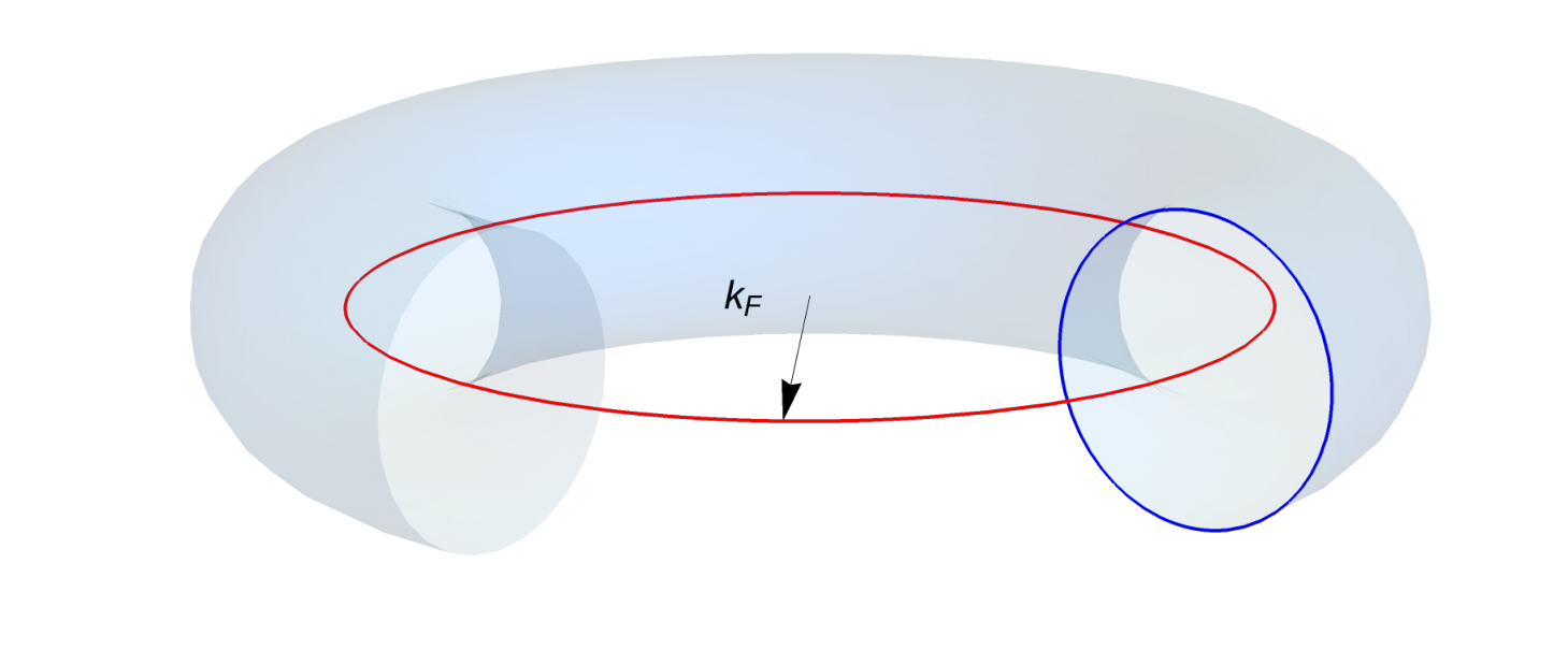
By making the circle discrete as above, we can define the discrete Berry phase

where $|n_{i_{1}}\rangle$ and $|n_{i_{2}}\rangle$ are eigenstates at two adjacent discrete points $i_{1}$ and $i_{2}$ along the path. The total Berry phase along the closed path is then the summation of all the discrete phases.

When $k_{y}=0$ from the Lagrangian (2.5) and the parameters we chose above, we have the eigenstates

and the associated energy eigenvalues $E^{I}=-\sqrt{(k_{x}-2)^{2}+k_{z}^{2}}$,  $E^{II}=\sqrt{(k_{x}-2)^{2}+k_{z}^{2}}$. For the choice of the “discrete” circle with (4.1), we have either states with energy $-l$ or $l$. By substituting (4.1) and (4.3) into (4.2) and do the summation of all the discrete phases, we find that the nontrivial phase factor is from the point where the normalized norm of two adjacent eigenstates becomes $-1$. For states with energy $-l$, i.e. $|n^{I}\rangle$, due to $\langle n^{I}(k_{x}=2+0_{-},k_{z}\simeq l)|n^{I}(k_{x}=2+0_{+},k_{z}\simeq l)\rangle<0$ we have a phase factor $\pi$ from (4.2). Similarly for states with energy $l$, i.e. $|n^{II}\rangle$, the phase factor $\pi$ of the Berry phase is due to $\langle n^{II}(k_{x}=2+0_{-},k_{z}\simeq-l)|n^{II}(k_{x}=2+0_{+},k_{z}\simeq-l)\rangle<0$. Therefore one concludes that Berry phase associated with a closed loop enclosing the node is $\pi$, which means that the nodal line semimetal described by (2.5) is topologically nontrivial.

References

- [1] A. A. Burkov, Weyl metals, Annu. Rev. Condens. Matter Phys. 9, 359 (2018) [arXiv:1704.06660]
- [2] N. P. Armitage, E. J. Mele, A. Vishwanath, Weyl and Dirac semimetals in three-dimensional solids, Rev. Mod. Phys. 90, 15001 (2018), [arXiv:1705.01111].
- [3] C. Fang, H. Weng, X. Dai and Z. Fang, Topological nodal line semimetals, Chin. Phys. B 25, 117106 (2016) [arXiv:1609.05414].
- [4] J. Zaanen, Y. W. Sun, Y. Liu and K. Schalm, Holographic Duality in Condensed Matter Physics, Cambridge University Press, 2015.
- [5] M. Ammon and J. Erdmenger, Gauge/gravity duality: Foundations and applications, Cambridge University Press, 2015.
- [6] S. A. Hartnoll, A. Lucas and S. Sachdev, Holographic quantum matter, [arXiv:1612.07324], MIT Press, 2017.
- [7] K. Landsteiner and Y. Liu, The holographic Weyl semi-metal, Phys. Lett. B 753, 453-457 (2016) [arXiv:1505.04772].
- [8]
Y. Liu and Y. W. Sun,
Topological nodal line semimetals in holography,
JHEP 12 (2018), 072
[arXiv:1801.09357].
Y. Liu and Y. W. Sun, Topological invariants for holographic semimetals, JHEP 10, 189 (2018) [arXiv:1809.00513]. - [9] K. Landsteiner, Y. Liu and Y. W. Sun, Quantum phase transition between a topological and a trivial semimetal from holography, Phys. Rev. Lett. 116, no.8, 081602 (2016) [arXiv:1511.05505].
- [10] K. Landsteiner, Y. Liu and Y. W. Sun, Odd viscosity in the quantum critical region of a holographic Weyl semimetal, Phys. Rev. Lett. 117, no.8, 081604 (2016) [arXiv:1604.01346].
- [11] C. Copetti, J. Fernández-Pendás and K. Landsteiner, Axial Hall effect and universality of holographic Weyl semi-metals, JHEP 02, 138 (2017) [arXiv:1611.08125].
- [12] G. Grignani, A. Marini, F. Pena-Benitez and S. Speziali, AC conductivity for a holographic Weyl Semimetal, JHEP 03, 125 (2017) [arXiv:1612.00486].
- [13] M. Ammon, M. Heinrich, A. Jiménez-Alba and S. Moeckel, Surface States in Holographic Weyl Semimetals, Phys. Rev. Lett. 118, no.20, 201601 (2017) [arXiv:1612.00836].
- [14] M. Ammon, M. Baggioli, A. Jiménez-Alba and S. Moeckel, A smeared quantum phase transition in disordered holography, JHEP 04, 068 (2018) [arXiv:1802.08650].
- [15] M. Baggioli, B. Padhi, P. W. Phillips and C. Setty, Conjecture on the Butterfly Velocity across a Quantum Phase Transition, JHEP 07, 049 (2018) [arXiv:1805.01470].
- [16] Y. Liu and J. Zhao, Weyl semimetal/insulator transition from holography, JHEP 12, 124 (2018) [arXiv:1809.08601].
- [17] G. Song, J. Rong and S. J. Sin, Stability of topology in interacting Weyl semi-metal and topological dipole in holography, JHEP 10, 109 (2019) [arXiv:1904.09349].
- [18] X. Ji, Y. Liu and X. M. Wu, Chiral vortical conductivity across a topological phase transition from holography, Phys. Rev. D 100, no.12, 126013 (2019) [arXiv:1904.08058].
- [19] I. Tanaka, Holographic quantum singularity, [arXiv:2001.06611].
- [20] V. Juričić, I. Salazar Landea and R. Soto-Garrido, Phase transitions in a holographic multi-Weyl semimetal, JHEP 07, 052 (2020) [arXiv:2005.10387].
- [21] M. Baggioli and D. Giataganas, Detecting Topological Quantum Phase Transitions via the c-Function, [arXiv:2007.07273].
- [22] B. Kiczek, M. Rogatko and K. I. Wysokiński, Anomalous Hall conductivity of the holographic Dirac semimetals, [arXiv:2010.13095].
- [23] U. Gursoy, V. Jacobs, E. Plauschinn, H. Stoof and S. Vandoren, Holographic models for undoped Weyl semimetals, JHEP 04, 127 (2013) [arXiv:1209.2593].
- [24] K. B. Fadafan, A. O’ Bannon, R. Rodgers, M. Russell, A Weyl Semimetal from AdS/CFT with Flavour, [arXiv:2012.11434].
- [25] K. Landsteiner, Y. Liu and Y. W. Sun, Holographic topological semimetals, Sci. China Phys. Mech. Astron. 63 (2020) no.5, 250001 [arXiv:1911.07978].
- [26] R. Alvares, C. Hoyos and A. Karch, An improved model of vector mesons in holographic QCD, Phys. Rev. D 84, 095020 (2011) [arXiv:1108.1191].
- [27] A. A. Burkov, M. D. Hook and L. Balents, Topological nodal semimetals, Phys. Rev. B 84, 235126 (2011) [arXiv:1110.1089].
- [28] S. K. Domokos, J. A. Harvey and A. B. Royston, Completing the framework of AdS/QCD: mesons and excited , JHEP 05 (2011), 107 [arXiv:1101.3315].
- [29] M. V. Berry, Quantal phase factors accompanying adiabatic changes, Proc. R. Soc. Lond. A3924557.
- [30] M. Cubrovic, J. Zaanen and K. Schalm, String Theory, Quantum Phase Transitions and the Emergent Fermi-Liquid, Science 325 (2009), 439-444 [arXiv:0904.1993].
- [31] H. Liu, J. McGreevy and D. Vegh, Non-Fermi liquids from holography, Phys. Rev. D 83 (2011), 065029 [arXiv:0903.2477].
- [32] N. Iqbal and H. Liu, Real-time response in AdS/CFT with application to spinors, Fortsch. Phys. 57 (2009), 367-384 [arXiv:0903.2596].
- [33] S. S. Gubser, F. D. Rocha and A. Yarom, Fermion correlators in non-abelian holographic superconductors, JHEP 11 (2010), 085 [arXiv:1002.4416].
- [34] M. Ammon, J. Erdmenger, M. Kaminski and A. O’Bannon, Fermionic Operator Mixing in Holographic p-wave Superfluids, JHEP 05 (2010), 053 [arXiv:1003.1134].
- [35] N. W. M. Plantz, F. García Flórez and H. T. C. Stoof, Massive Dirac fermions from holography, JHEP 04, 123 (2018) [arXiv:1802.04191].
- [36] Z. Wang and S. C. Zhang, Simplified topological invariants for interacting insulators, Phys. Rev. X 2 (2012), 031008 [arXiv:1203.1028].
- [37] Z. Wang and B. Yan, Topological Hamiltonian as an Exact Tool for Topological Invariants, J. Phys. : Condens. Matter 25 (2013), 155601 [arXiv:1207.7341].
- [38] S. A. Hartnoll, D. M. Hofman and D. Vegh, Stellar spectroscopy: Fermions and holographic Lifshitz criticality, JHEP 08 (2011), 096 [arXiv:1105.3197].
- [39] N. Iqbal, H. Liu and M. Mezei, Semi-local quantum liquids, JHEP 04 (2012), 086 [arXiv:1105.4621].
- [40] M. Cubrovic, Y. Liu, K. Schalm, Y. W. Sun and J. Zaanen, Spectral probes of the holographic Fermi groundstate: dialing between the electron star and AdS Dirac hair, Phys. Rev. D 84 (2011), 086002 [arXiv:1106.1798].
- [41] T. Faulkner and J. Polchinski, Semi-Holographic Fermi Liquids, JHEP 06 (2011), 012 [arXiv:1001.5049].
- [42] M. Moore, P. Surówka, V. Juričić and B. Roy, Shear viscosity as a probe of nodal topology, Phys. Rev. B 101 (2020) no.16, 161111 [arXiv:1912.07611].
- [43] K. Landsteiner, Notes on Anomaly Induced Transport, Acta Phys. Polon. B 47, 2617 (2016) [arXiv:1610.04413].
- [44] M. Ammon, S. Grieninger, A. Jimenez-Alba, R. P. Macedo and L. Melgar, Holographic quenches and anomalous transport, JHEP 09 (2016), 131 [arXiv:1607.06817].
- [45] Y. Bu, T. Demircik and M. Lublinsky, Nonlinear chiral transport from holography, JHEP 01, 078 (2019) [arXiv:1807.08467].
- [46] M. Haack, D. Sarkar and A. Yarom, Probing anomalous driving, JHEP 04, 034 (2019) [arXiv:1812.08210].
- [47] M. Ammon, S. Grieninger, J. Hernandez, M. Kaminski, R. Koirala, J. Leiber and J. Wu, Chiral hydrodynamics in strong magnetic fields, [arXiv:2012.09183].
- [48] M. Henneaux, Boundary terms in the AdS / CFT correspondence for spinor fields, [arXiv:hep-th/9902137].
- [49] J. N. Laia and D. Tong, A Holographic Flat Band, JHEP 11 (2011), 125 [arXiv:1108.1381].