跳到论文正文
W Papers独立论文阅读器 arXiv:2012.12574 论文正文 计算阅读时间 · 0%
引用这篇论文根据当前论文元数据生成,正式投稿前建议核对。


License: CC BY-NC-ND 4.0
arXiv:2012.12574v1 [math.AP] 23 Dec 2020

Long time confinement of vorticity around a stable stationary point vortex in a bounded planar domain

Martin Donati    Drago s , Iftimie
Abstract

In this paper we consider the incompressible Euler equation in a simply-connected bounded planar domain. We study the confinement of the vorticity around a stationary point vortex. We show that the power law confinement around the center of the unit disk obtained in [2] remains true in the case of a stationary point vortex in a simply-connected bounded domain. The domain and the stationary point vortex must satisfy a condition expressed in terms of the conformal mapping from the domain to the unit disk. Explicit examples are discussed at the end.

1 Introduction and main result

To study the behavior of an incompressible inviscid fluid, we consider the planar Euler equations in a bounded domain Ω⊂ℝ2\Omega\subset\mathbb{R}^{2}:

{∂tu⁡(x,t)+u⁡(x,t)⋅∇u​(x,t)=−∇p​(x,t),∀(x,t)∈Ω×ℝ+∗u⁡(x,0)=u0​(x),∀x∈Ω∇⋅u⁡(x,t)=0,∀(x,t)∈Ω×ℝ+u⁡(x,t)⋅n→=0,∀(x,t)∈∂Ω×ℝ+\begin{cases}\partial_{t}u(x,t)+u(x,t)\cdot\nabla u(x,t)=-\nabla p(x,t),&\forall(x,t)\in\Omega\times\mathbb{R}^{*}_{+}\\ u(x,0)=u_{0}(x),&\forall x\in\Omega\\ \nabla\cdot u(x,t)=0,&\forall(x,t)\in\Omega\times\mathbb{R}_{+}\\ u(x,t)\cdot\vec{n}=0,&\forall(x,t)\in\partial\Omega\times\mathbb{R}_{+}\end{cases} (1.1)

where uu denotes the velocity of the fluid, pp its internal pressure, and nn is the exterior normal to ∂Ω\partial\Omega. If Ω=ℝ2\Omega=\mathbb{R}^{2} the boundary condition should be changed into a vanishing condition at infinity. We define the fluid’s vorticity by ω=∂1u2−∂2u1\omega=\partial_{1}u_{2}-\partial_{2}u_{1}, which satisfies the equation:

∂tω⁡(x,t)+u⁡(x,t)⋅∇ω​(x,t)=0.\partial_{t}\omega(x,t)+u(x,t)\cdot\nabla\omega(x,t)=0. (1.2)

If the domain Ω\Omega is smooth, then we have a unique global smooth solution of (1.1), see [17]. In addition, if ∂Ω∈C1,1\partial\Omega\in C^{1,1} we have the following result due to Yudovitch (see [18]): for any ω0∈L1∩L∞\omega_{0}\in L^{1}\cap L^{\infty}, there exists a unique solution to (1.1), with u∈L∞​(ℝ+,W1,p)u\in L^{\infty}(\mathbb{R}^{+},W^{1,p}), for every 1<p<∞1<p<\infty, and ω∈L∞​(ℝ+,L1∩L∞)\omega\in L^{\infty}(\mathbb{R}^{+},L^{1}\cap L^{\infty}). The result is true in more general domains, in particular in domains with finite number of corners with angle strictly less than π\pi and when the vorticity is compactly supported in Ω\Omega, see [13] and [6]. In particular, one could take Ω\Omega to be a convex polygon.

Let us denote by GΩG_{\Omega} the Green’s function of Ω\Omega. Since the domain is supposed to be simply-connected, the velocity can be recovered from the vorticity through the following Biot-Savart law

u⁡(x,t)=∫Ω∇x⟂​GΩ​(x,y)​ω​(y,t)​𝑑y,u(x,t)=\int_{\Omega}\nabla^{\perp}_{x}G_{\Omega}(x,y)\omega(y,t)\,\mathrm{d}y, (1.3)

where x⟂=(−x2,x1)x^{\perp}=(-x_{2},x_{1}).

The point vortex system is a simplified version of the Euler equations where the vorticity is assumed to be a finite sum of Dirac masses ω0=∑i=1Nai​δzi\omega_{0}=\sum_{i=1}^{N}a_{i}\delta_{z_{i}}. It was introduced by Helmholtz in [8], see also [15]. Since (1.2) is a transport equation, one expects the vorticity to remain a sum of Dirac masses at some points zi​(t)z_{i}(t). The Biot-Savart law (1.3) reads in this case

u⁡(x,t)=∑i=1Nai​∇x⟂GΩ​(x,zi​(t)).u(x,t)=\sum_{i=1}^{N}a_{i}\nabla_{x}^{\perp}G_{\Omega}(x,z_{i}(t)).

However, if xx is one of the points zi​(t)z_{i}(t), then this velocity is not defined as GΩ​(x,y)G_{\Omega}(x,y) is singular at y=xy=x. But as xx approaches zi​(t)z_{i}(t), the singular part of the velocity defined above is given by fast rotation around that point. More precisely, since the map GΩ−Gℝ2G_{\Omega}-G_{\mathbb{R}^{2}} is harmonic in both its variable on Ω\Omega, the function γΩ:Ω×Ω→ℝ\gamma_{\Omega}:\Omega\times\Omega\rightarrow\mathbb{R}, γΩ=GΩ−Gℝ2=GΩ−12​π​ln⁡|x−y|\gamma_{\Omega}=G_{\Omega}-G_{\mathbb{R}^{2}}=G_{\Omega}-\frac{1}{2\pi}\ln|x-y| is smooth. So the singular part of ∇x⟂GΩ​(x,zi​(t))\nabla_{x}^{\perp}G_{\Omega}(x,z_{i}(t)) is given by (x−zi)⟂2​π​|x−zi|2\frac{(x-z_{i})^{\perp}}{2\pi|x-z_{i}|^{2}}. The point vortex system consists in ignoring this singular part which should have no influence on the motion of ziz_{i} itself. Denoting by γ~Ω​(x)=γ⁡(x,x)\widetilde{\gamma}_{\Omega}(x)=\gamma(x,x) the Robin function of the domain Ω\Omega we obtain then the following point vortex dynamic:

∀1≤i≤N,d​zi​(t)d​t=∑j=1j≠iNaj​∇x⟂GΩ​(zi​(t),zj​(t))+ai​12​∇⟂γ~Ω​(zi​(t)),\forall 1\leq i\leq N,\hskip 5.69046pt\frac{\,\mathrm{d}z_{i}(t)}{\,\mathrm{d}t}=\sum_{\begin{subarray}{c}j=1\\ j\neq i\end{subarray}}^{N}a_{j}\nabla_{x}^{\perp}G_{\Omega}(z_{i}(t),z_{j}(t))+a_{i}\frac{1}{2}\nabla^{\perp}\widetilde{\gamma}_{\Omega}(z_{i}(t)), (1.4)

where the (ai)1≤i≤N∈ℝ∖{0}(a_{i})_{1\leq i\leq N}\in\mathbb{R}\setminus\{0\} are the masses of the point vortices (zi​(t))1≤i≤N(z_{i}(t))_{1\leq i\leq N}. Equations (1.4) are called Kirchhoff-Routh equations.

Due to the singularities of the Green’s function, these equations are valid only while the points zi​(t)z_{i}(t) stay distinct and do not leave the domain Ω\Omega. There exist configurations leading to collapse of the point vortices, but they are exceptional, see [15] for the case of ℝ2\mathbb{R}^{2}, and [14] for the case of the unit disk (we will discuss this more in detail later).

An important question in fluid dynamics is whether the point vortex system is a good approximation of the Euler equations. There are convergence results in both ways.

Let us first mention that the point vortex system was used as a numerical approximation of the Euler system. More precisely, consider a smooth solution of the Euler equations and construct an initial discrete vorticity which is a sum of Dirac masses located on a grid (h​j)j∈ℤ2(hj)_{j\in\mathbb{Z}^{2}} where h∈ℝh\in\mathbb{R} is the length of the grid, with masses h2​ω0​(h​j)h^{2}\omega_{0}(hj). Solve then the point vortex system with this initial vorticity. In [4], the authors proved that this point vortex method is consistent, stable, and converges to the smooth solution of the Euler equation.

The convergence from the Euler system to the point vortex system was also proved in [16]. More precisely, consider a smooth initial vorticity that is sharply concentrated around some initial point vortices ziz_{i}: the support of ω0\omega_{0} is included in the union of the disks of radius ε\varepsilon around the points ziz_{i}, with ε>0\varepsilon>0 being small. The authors of [16] proved that for any time τ\tau, and for any δ>0\delta>0, if ε=ε⁡(τ,δ)>0\varepsilon=\varepsilon(\tau,\delta)>0 is small enough then the solution stays sharply concentrated within disks of radius δ\delta from the points zi​(t)z_{i}(t) up to time τ\tau. This statement can be seen as a fixed time confinement result.

In this paper we are interested in the so-called long time confinement problem, that is we want to know for how long confinement around point vortices remains true. More precisely, we want to understand how ε\varepsilon, δ\delta and τ\tau are linked together and we wish to obtain a confinement time τ\tau as large as possible. We already know from [16] that τ\tau goes to infinity when ε\varepsilon goes to 0, but we would like to obtain an explicit rate as good as possible.

This problem was already studied by Buttà and Marchioro [2]. These authors assumed that δ=εβ\delta=\varepsilon^{\beta}, with β<1/2\beta<1/2, and made the following assumptions on the initial vorticity. Assume that ω0∈L1∩L∞\omega_{0}\in L^{1}\cap L^{\infty} and there exists ν\nu such that

{|ω0|≤ε−νω0=∑i=1Nω0,i,supp⁡ω0,i⊂D⁡(zi,ε)ω0,i​ has a definite sign∫Ωω0,i​dx=ai.\begin{cases}|\omega_{0}|\leq\varepsilon^{-\nu}\\ \displaystyle\omega_{0}=\sum_{i=1}^{N}\omega_{0,i},\hskip 5.69046pt\operatorname{supp}\omega_{0,i}\subset D(z_{i},\varepsilon)\\ \omega_{0,i}\text{ has a definite sign}\\ \displaystyle\int_{\Omega}\omega_{0,i}\,\mathrm{d}x=a_{i}.\end{cases} (1.5)

Let ω⁡(x,t)\omega(x,t) the solution of (1.2).

We denote by τε,β\tau_{\varepsilon,\beta} the exit time of the vorticity from the disks of radius εβ\varepsilon^{\beta}:

τε,β=sup{t≥0,∀s∈[0,t],suppω(⋅,s)⊂⋃i=1ND(zi(s),εβ)}.\tau_{\varepsilon,\beta}=\sup\left\{t\geq 0,\forall s\in[0,t],\operatorname{supp}\omega(\cdot,s)\subset\bigcup_{i=1}^{N}D(z_{i}(s),\varepsilon^{\beta})\right\}. (1.6)

For any NN-tuple of distinct points (zi)∈Ω(z_{i})\in\Omega, there exists ε\varepsilon small enough, such that the disks D⁡(zi​(0),εβ)D(z_{i}(0),\varepsilon^{\beta}) are disjoints, and therefore this exit time is well defined and strictly positive. The aim is to obtain a lower bound on τε,β\tau_{\varepsilon,\beta} depending explicitly on ε\varepsilon. Two results have been obtained in [2]. The first is a logarithmic confinement for the whole plane.

Theorem 1.1 ([2]).

Assume that Ω=ℝ2\Omega=\mathbb{R}^{2}, that the initial vorticity satisfies (1.5) and that the point vortex system with initial data ∑i=1nai​δzi\sum_{i=1}^{n}a_{i}\delta_{z_{i}} has a global solution. Then for every β<1/2\beta<1/2 there exists ε0>0\varepsilon_{0}>0 and C>0C>0 such that

∀ε⁡<ε0,τε,β>​C​|ln⁡(ε)|.\forall\varepsilon<\varepsilon_{0},\hskip 5.69046pt\tau_{\varepsilon,\beta}>C|\ln(\varepsilon)|.

The second result is more restrictive, it holds true for the unit disk and for a single point vortex located at the center, but the conclusion is much stronger since it gives a power-law confinement.

Theorem 1.2 ([2]).

Let Ω=D\Omega=D and ω0\omega_{0} satisfying (1.5) with N=1N=1 and z1=0z_{1}=0, so that it is compactly supported within the disk D⁡(0,ε)D(0,\varepsilon). Then for every β<1/2\beta<1/2 there exists ε0>0\varepsilon_{0}>0 and α>0\alpha>0 such that:

∀ε⁡<ε0,τε,β>​ε−α.\forall\varepsilon<\varepsilon_{0},\hskip 5.69046pt\tau_{\varepsilon,\beta}>\varepsilon^{-\alpha}.

The aim of this paper is to extend Theorem 1.2 to more general domains. We also observe that Theorem 1.1 can also be extended to bounded domains; we will discuss this problem in a forthcoming paper.

We consider a single point vortex in a simply-connected bounded domain. We assume for simplicity that the mass of the point vortex is 1, but the results below hold true for a general mass. The first question that arises is the location of the point vortex. We will show that there are special points that allow us to obtain the power-law lower bound while for others the logarithmic bound is probably optimal.

The dynamic of a single point vortex of mass aa reduces to the following ODE

dd​t​z​(t)=a​12​∇⟂γ~Ω​(z⁡(t)).\frac{\,\mathrm{d}}{\,\mathrm{d}t}z(t)=a\frac{1}{2}\nabla^{\perp}\widetilde{\gamma}_{\Omega}(z(t)).

It is obvious from this ODE that a point vortex is stationary if and only if it is a critical point of the Robin function γ~\widetilde{\gamma}. The Robin function has been studied, see [5], and we know that such critical points always exist in a bounded domain. Let x0x_{0} be a critical point of the Robin function which is fixed for the rest of this paper. From the Riemann mapping theorem we know that there exists a biholomorphic map TT from Ω\Omega to the unit disk DD. We can chose TT such that it maps x0x_{0} to 0: T⁡(x0)=0T(x_{0})=0. We shall see below that x0x_{0} is a critical point of the Robin function if and only if T′′​(x0)=0T^{\prime\prime}(x_{0})=0 (see Proposition 2.4). This condition therefore characterizes the fact that x0x_{0} is a stationary point for the point vortex system. We call such points stationary points.

Our main result is the following.

Theorem 1.3.

Let Ω\Omega be a simply connected bounded domain of ℝ2\mathbb{R}^{2} with C1,1C^{1,1} boundary. Let x0x_{0} be a stationary point such that T′′′​(x0)=0T^{\prime\prime\prime}(x_{0})=0 where TT is a biholomorphism from Ω\Omega to the unit disk, mapping x0x_{0} to 0. Assume that ω0\omega_{0} satisfies (1.5) with N=1N=1 and z1=x0z_{1}=x_{0}. Then for every β<1/2\beta<1/2 and for any α<min⁡(β,2−4​β)\alpha<\min(\beta,2-4\beta), there exists ε0>0\varepsilon_{0}>0 such that

∀ε⁡<ε0,τε,β>​ε−α.\forall\varepsilon<\varepsilon_{0},\hskip 5.69046pt\tau_{\varepsilon,\beta}>\varepsilon^{-\alpha}.

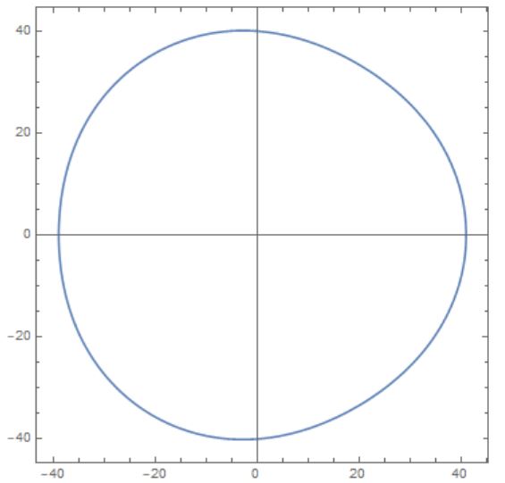
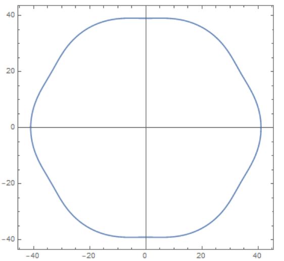
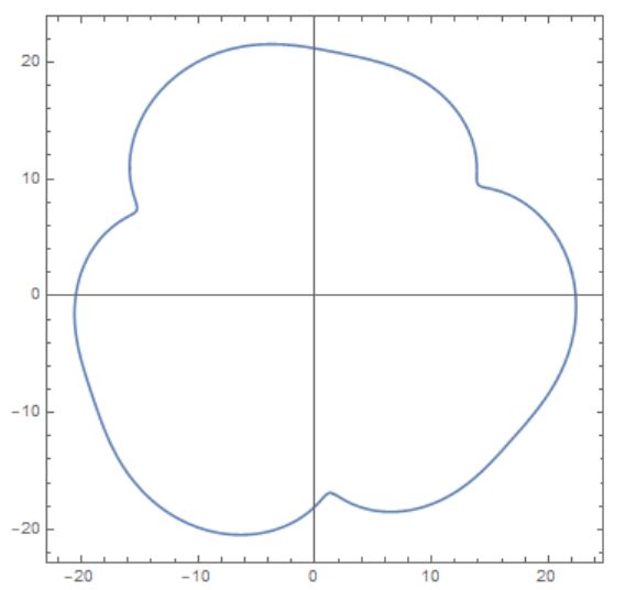
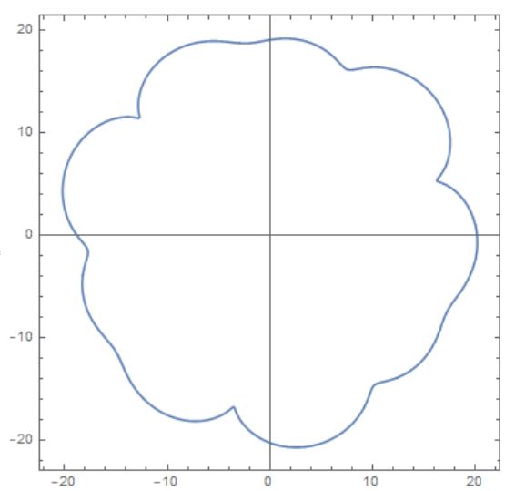
This extends Theorem 1.2 to more general bounded domains. Indeed, in the case of the unit disk we can choose T⁡(z)=zT(z)=z so the hypothesis given above is verified for the center of the disk. Let us also observe that the hypothesis that x0x_{0} is stationary induces no restriction on the domain Ω\Omega. Indeed, we recall that Gustafsson [5] proved that every simply-connected smooth domain has at least a stationary point. However, the hypothesis that T′′′​(x0)=0T^{\prime\prime\prime}(x_{0})=0 is a condition that not all domains satisfy. We will comment on this in the last section. We will see in particular that any domain which is invariant by some rotation of angle θ∈(0,π)\theta\in(0,\pi) around x0x_{0} satisfies the condition T′′′​(x0)=0T^{\prime\prime\prime}(x_{0})=0.

In order to understand better the significance of the condition T′′′​(x0)=0T^{\prime\prime\prime}(x_{0})=0, one could assume that the vorticity ω\omega itself is a point vortex. We study in detail this perturbation problem in Section 3. We will prove there that if |T′′′​(x0)|<2​|T′​(x0)|3|T^{\prime\prime\prime}(x_{0})|<2|T^{\prime}(x_{0})|^{3} then τε,β=∞\tau_{\varepsilon,\beta}=\infty if ε\varepsilon is small enough while if |T′′′​(x0)|>2​|T′​(x0)|3|T^{\prime\prime\prime}(x_{0})|>2|T^{\prime}(x_{0})|^{3} then τε,β\tau_{\varepsilon,\beta} is in general not better than C​|ln⁡ε|C|\ln\varepsilon|, see Theorem 3.1. In other words, in this particular case we have long time confinement better than C​|ln⁡ε|C|\ln\varepsilon| if and only if |T′′′​(x0)|<2​|T′​(x0)|3|T^{\prime\prime\prime}(x_{0})|<2|T^{\prime}(x_{0})|^{3}. However, when ω\omega is smooth we require the stronger assumption T′′′​(x0)=0T^{\prime\prime\prime}(x_{0})=0.

The plan of the paper is the following. In Section 2 we introduce some notation and discuss some facts about the Green’s function and the point vortex system. In section 3 we consider the particular case when ω\omega is a point vortex itself. In Section 4 we prove Theorem 1.3. The last section contains some final remarks and some examples of domains for which our theorem applies.

2 Preliminary tools

List of notation:

  • •

    Ω\Omega is a C1,1C^{1,1} bounded and simply connected domain of ℝ2\mathbb{R}^{2};

  • •

    D⁡(x0,r)D(x_{0},r) is the disk of center x0x_{0} and of radius rr and D=D⁡(0,1)D=D(0,1);

  • •

    uu is the velocity of the fluid and pp its pressure, satisfying equations (1.1);

  • •

    ω=∂1u2−∂2u1\omega=\partial_{1}u_{2}-\partial_{2}u_{1} is the vorticity of the fluid;

  • •

    supp⁡f\operatorname{supp}f is the support of the function ff, namely the closure of the set {x∈Ω,f⁡(x)≠0}\{x\in\Omega,f(x)\neq 0\};

  • •

    δz\delta_{z} is the Dirac mass in zz;

  • •

    GΩG_{\Omega} or GG is the Green’s function of the domain Ω\Omega;

  • •

    γΩ\gamma_{\Omega} or γ\gamma is the regular part of GΩG_{\Omega}, see relation (2.1);

  • •

    γ~Ω​(x)=γΩ​(x,x)\widetilde{\gamma}_{\Omega}(x)=\gamma_{\Omega}(x,x) is the Robin function;

  • •

    C,C1,C2,…;K,K1,K2,…,LC,C_{1},C_{2},\ldots;K,K_{1},K_{2},\ldots,L, are strictly positive constants that may vary from one line to another, when their value is not important to the result;

  • •

    a⋅ba\cdot b is the scalar product of vectors in ℝ2\mathbb{R}^{2};

  • •

    ∇f\nabla f, D2​fD^{2}f and ∇⋅g\nabla\cdot g are respectively the gradient of ff, its Hessian matrix, and the divergence of gg.

2.1 Green’s Function

We recall that the Green’s function of a domain Ω\Omega is the solution of

Δx​GΩ​(x,y)=δ⁡(x−y)\Delta_{x}G_{\Omega}(x,y)=\delta(x-y)

vanishing at the boundary, and at infinity if Ω\Omega is unbounded. It is a symmetric function on Ω2\Omega^{2} that satisfies for x≠yx\neq y

Δx​(GΩ​(x,y)−Gℝ2​(x,y))=0,\Delta_{x}(G_{\Omega}(x,y)-G_{\mathbb{R}^{2}}(x,y))=0,

which means that GΩ−Gℝ2G_{\Omega}-G_{\mathbb{R}^{2}} is a function, denoted by γΩ\gamma_{\Omega}, which is harmonic in both of its variable. Therefore, we have:

GΩ​(x,y)=12​π​ln⁡|x−y|+γΩ​(x,y)G_{\Omega}(x,y)=\frac{1}{2\pi}\ln|x-y|+\gamma_{\Omega}(x,y) (2.1)

where γΩ\gamma_{\Omega} is symmetric and smooth.

In the particular case of Ω=D\Omega=D, we have that

GD​(x,y)=ln⁡|x−y|2​π−ln⁡|x−y∗|​|y|2​πG_{D}(x,y)=\frac{\ln|x-y|}{2\pi}-\frac{\ln|x-y^{*}||y|}{2\pi} (2.2)

where y∗=y|y|2\displaystyle y^{*}=\frac{y}{|y|^{2}} is the inverse relative to the unit circle. In particular,

γD​(x,y)=−ln⁡|x−y∗|​|y|2​π.\gamma_{D}(x,y)=-\frac{\ln|x-y^{*}||y|}{2\pi}. (2.3)

Let x0∈Ωx_{0}\in\Omega. From the Riemann Mapping Theorem (see for instance [1], chapter 6) and recalling that Ω\Omega is simply-connected, we know that there exists a biholomorphic map TT from Ω\Omega to the unit disk DD. The map TT is unique up to compositions with the biholomorphisms of the unit disk which are given by

ϕz0,λ​(z)=λ​z0−z1−z0¯​z,\phi_{z_{0},\lambda}(z)=\lambda\frac{z_{0}-z}{1-\overline{z_{0}}z},

with z0∈Dz_{0}\in D and |λ|=1|\lambda|=1 arbitrary. Choosing z0z_{0} and λ\lambda conveniently, we can assume without loss of generality that T⁡(x0)=0T(x_{0})=0 and that T′​(x0)T^{\prime}(x_{0}) is a strictly positive real number. These two conditions insure the uniqueness of the conformal map TT. Let us observe that in Theorem 1.3 the mapping TT is not unique since we only assume that it maps x0x_{0} to 0. However, the condition T′′′​(x0)=0T^{\prime\prime\prime}(x_{0})=0 does not depend on the choice of TT (once we assumed that it maps x0x_{0} to 0). Indeed, if T1T_{1} and T2T_{2} are two biholomorphisms from Ω\Omega to DD mapping x0x_{0} to 0, then T1∘T2−1T_{1}\circ T_{2}^{-1} is a biholomorphism from DD to DD mapping 0 to 0. So it must be a rotation: there exists some λ\lambda of modulus 1 such that T1∘T2−1​(z)=λ​zT_{1}\circ T_{2}^{-1}(z)=\lambda z. So T1=λ​T2T_{1}=\lambda T_{2} and therefore T1′′′​(x0)=λ​T2′′′​(x0)T_{1}^{\prime\prime\prime}(x_{0})=\lambda T_{2}^{\prime\prime\prime}(x_{0}). Then T1′′′​(x0)=0T_{1}^{\prime\prime\prime}(x_{0})=0 if and only if T2′′′​(x0)=0T_{2}^{\prime\prime\prime}(x_{0})=0.

We will assume from now on that T⁡(x0)=0T(x_{0})=0. The assumption that T′​(x0)>0T^{\prime}(x_{0})>0 can be made but is not necessary. In the following, T′​(x0)T^{\prime}(x_{0}) is a complex number.

The properties of the conformal map TT imply a precise description of the Green’s function of Ω\Omega. Indeed, a Green’s function composed with a conformal mapping is another Green’s function, see for example [1] chapter 6. Therefore the formula (2.2) yields the following proposition.

Proposition 2.1.

Let TT be the biholomorphic mapping introduced above. Then

GΩ​(x,y)=GD​(T⁡(x),T⁡(y))=ln⁡|T⁡(x)−T⁡(y)|2​π−ln⁡|T⁡(x)−T​(y)∗|​|T​(y)∗|2​π.G_{\Omega}(x,y)=G_{D}(T(x),T(y))=\frac{\ln|T(x)-T(y)|}{2\pi}-\frac{\ln|T(x)-T(y)^{*}||T(y)^{*}|}{2\pi}.

In the following, we will have to use both characterizations of the map TT, as a ℂ→ℂ\mathbb{C}\rightarrow\mathbb{C} map, and as a ℝ2→ℝ2\mathbb{R}^{2}\rightarrow\mathbb{R}^{2} map. In particular, we recall that T′​(x)=∂1T⁡(x)=∂1T1​(x)+i​∂1T2​(x)T^{\prime}(x)=\partial_{1}T(x)=\partial_{1}T_{1}(x)+i\partial_{1}T_{2}(x), and that ∂1T1=∂2T2\partial_{1}T_{1}=\partial_{2}T_{2} and ∂2T1=−∂1T2\partial_{2}T_{1}=-\partial_{1}T_{2}. So for any map f∈C1​(ℝ2,ℝ)f\in C^{1}(\mathbb{R}^{2},\mathbb{R}), we have that

∇(f∘T)​(x)=(∂1T1​(x)​∂1f⁡(T⁡(x))+∂1T2​(x)​∂2f⁡(T⁡(x))−∂1T2(x)∂1f(T(x))+∂1T1(x)∂2f(T(x))),\nabla(f\circ T)(x)=\begin{pmatrix}\partial_{1}T_{1}(x)\partial_{1}f(T(x))+\partial_{1}T_{2}(x)\partial_{2}f(T(x))\\ -\partial_{1}T_{2}(x)\partial_{1}f(T(x))+\partial_{1}T_{1}(x)\partial_{2}f(T(x))\end{pmatrix},

or as complex numbers:

∂1(f∘T)​(x)+i​∂2(f∘T)​(x)\displaystyle\partial_{1}(f\circ T)(x)+i\partial_{2}(f\circ T)(x) =Re⁡(T′​(x))​∂1f⁡(T⁡(x))+Im⁡(T′​(x))​∂2f⁡(T⁡(x))\displaystyle=\operatorname{Re}(T^{\prime}(x))\partial_{1}f(T(x))+\operatorname{Im}(T^{\prime}(x))\partial_{2}f(T(x))
+i[−Im(T′(x))∂1f(T(x))+Re(T′(x))∂2f(T(x))]\displaystyle\hskip 5.69046pt\hskip 5.69046pt\hskip 5.69046pt+i[-\operatorname{Im}(T^{\prime}(x))\partial_{1}f(T(x))+\operatorname{Re}(T^{\prime}(x))\partial_{2}f(T(x))]
=T′​(x)¯​(∂1f⁡(T⁡(x))+i​∂2f⁡(T⁡(x))).\displaystyle=\overline{T^{\prime}(x)}(\partial_{1}f(T(x))+i\partial_{2}f(T(x))).

Identifying ∇f=∂1f+i​∂2f\nabla f=\partial_{1}f+i\partial_{2}f, we have:

∇(f∘T)(x)=T′​(x)¯∇f(T(x)),\nabla(f\circ T)(x)=\overline{T^{\prime}(x)}\nabla f(T(x)), (2.4)

where the product above must be understood as the product of two complex numbers. We will frequently use this property in the following.

From Proposition 2.1 and from relation (2.1) applied for Ω\Omega and for DD we get that

γΩ​(x,y)=γD​(T⁡(x),T⁡(y))+12​π​ln⁡|T⁡(x)−T⁡(y)||x−y|,\gamma_{\Omega}(x,y)=\gamma_{D}(T(x),T(y))+\frac{1}{2\pi}\ln\frac{|T(x)-T(y)|}{|x-y|},

and letting y→xy\to x we obtain at the level of Robin functions

∀x∈Ω,γ~Ω​(x)=γ~D​(T⁡(x))+12​π​ln⁡|T′​(x)|.\forall x\in\Omega,\hskip 5.69046pt\hskip 5.69046pt\widetilde{\gamma}_{\Omega}(x)=\widetilde{\gamma}_{D}(T(x))+\frac{1}{2\pi}\ln|T^{\prime}(x)|. (2.5)

Using the explicit expression of γD\gamma_{D}, see relation (2.3), we can compute the gradient of γΩ\gamma_{\Omega}:

∇xγΩ​(x,y)\displaystyle\nabla_{x}\gamma_{\Omega}(x,y) =T′¯​(x)​(T​(x)−T​(y))2​π​|T⁡(x)−T⁡(y)|2−T′¯​(x)​(T⁡(x)−T​(y)∗)2​π​|T⁡(x)−T​(y)∗|2−(x−y)2​π​|x−y|2\displaystyle=\frac{\overline{T^{\prime}}(x)(T(x)-T(y))}{2\pi|T(x)-T(y)|^{2}}-\frac{\overline{T^{\prime}}(x)(T(x)-T(y)^{*})}{2\pi|T(x)-T(y)^{*}|^{2}}-\frac{(x-y)}{2\pi|x-y|^{2}} (2.6)
=T′​(x)¯2​π​(T⁡(x)−T⁡(y))¯−T′​(x)¯2​π​(T⁡(x)−T​(y)∗)¯−12​π​(x−y)¯\displaystyle=\frac{\overline{T^{\prime}(x)}}{2\pi\overline{(T(x)-T(y))}}-\frac{\overline{T^{\prime}(x)}}{2\pi\overline{(T(x)-T(y)^{*})}}-\frac{1}{2\pi\overline{(x-y)}}

where we used relation (2.4).

The mapping γ~Ω:Ω→ℝ2\widetilde{\gamma}_{\Omega}:\Omega\rightarrow\mathbb{R}^{2}, that will be named only γ~\widetilde{\gamma} when there is no ambiguity, has been studied extensively in [5]. In particular, it was shown in that paper that −γ~Ω-\widetilde{\gamma}_{\Omega} is a super-harmonic function, that is that Δ​γ~Ω>0\Delta\widetilde{\gamma}_{\Omega}>0, and that it goes to infinity near the boundary like −12​π​ln⁡(d⁡(x,∂Ω))-\frac{1}{2\pi}\ln(d(x,\partial\Omega)). This implies that we have the following proposition (see [5]).

Proposition 2.2 ([5]).

For every bounded and simply connected open set Ω\Omega, there exists at least one point x0x_{0} where γ~\widetilde{\gamma} reaches its minimum.

Critical points of γ~Ω\widetilde{\gamma}_{\Omega} will be of special interest in the following. The proposition above implies the existence of a critical point of the Robin function. Moreover, if Ω\Omega is convex, then the critical point is also unique (see [5]). Though we will not use this result here, it may be interesting to keep this in mind, especially when looking for explicit examples.

2.2 Point vortex system

The point vortex dynamic, which is described by equations (1.4), can exhibit finite time blow-up of solutions. One scenario of blow-up is when two point vortices hit each other in finite time, meaning that there exists i≠ji\neq j and t<∞t<\infty such that zi​(t)=zj​(t)z_{i}(t)=z_{j}(t). This phenomena can happen, see for instance [15] or [10] for an example of finite-time collapse of a self similar evolution of point vortices. Another scenario for blow-up is when a point vortex hits the boundary. However, the finite time blow-up is exceptional in the case of the whole plane, see [15], and for the unit disk, see [14]. In those cases, the NN-dimensional Lebesgue measure of the set of initial positions that lead to a collapse is 0. The case of a more general bounded domain is an ongoing work.

Let us recall the convergence theorem obtained in [16], for configurations of point vortices that do not lead to finite-time blow-up:

Theorem 2.3 ([16]).

Let (ai,zi​(t))(a_{i},z_{i}(t)) be a global solution of the point vortex system (1.4). For every δ>0\delta>0 and for every time τ\tau, there exists ε>0\varepsilon>0 such that if ω0\omega_{0} satisfies (1.5) for some 0<ν<8/30<\nu<8/3, then the vorticity stays confined up to the time τ\tau in disks of radius δ\delta centered on zi​(t)z_{i}(t).

In addition, the authors of [3] proved that τε,β→+∞\tau_{\varepsilon,\beta}\rightarrow+\infty as ε\varepsilon goes to 0 for any β<1/3\beta<1/3 (recall that τε,β\tau_{\varepsilon,\beta} was defined in relation (1.6)). However, these theorems don’t say anything about how δ\delta depends on the time τ\tau, or conversely, for how long this confinement remains true, depending on ε\varepsilon.

For some explicit examples of point vortices we refer to [9].

As mentioned in the introduction, the stationary point vortices are the critical points of the Robin function. Indeed, the relation (1.4) with N=1N=1 reduces to

z′​(t)=a2​∇⟂γ~Ω​(z⁡(t)).z^{\prime}(t)=\frac{a}{2}\nabla^{\perp}\widetilde{\gamma}_{\Omega}(z(t)).

We refer to such a critical point x0x_{0} by saying that it is a stationary point vortex.

Those points can also be characterized in terms of the conformal mapping TT as zeroes of T′′T^{\prime\prime}.

Proposition 2.4.

The following conditions are equivalent:

  • (i)

    A single point vortex placed in x0x_{0} is stationary,

  • (ii)

    ∇γ~Ω​(x0)=0\nabla\widetilde{\gamma}_{\Omega}(x_{0})=0,

  • (iii)

    T′′​(x0)=0T^{\prime\prime}(x_{0})=0.

Proof.

This proposition was already proved in [5]. We recall the proof for the convenience of the reader.

We already observed that (i)(i) and (i​i)(ii) are equivalent. We only need to prove that (i​i)(ii) is equivalent to (i​i​i)(iii). From relations (2.5) and (2.4), and recalling that T′T^{\prime} can’t vanish in Ω\Omega, we deduce that

∇γ~Ω​(x)=∇γ~D​(T⁡(x))​T′​(x)¯+12​π​T′​(x)​T′′​(x)¯|T′​(x)|2.\nabla\widetilde{\gamma}_{\Omega}(x)=\nabla\widetilde{\gamma}_{D}(T(x))\overline{T^{\prime}(x)}+\frac{1}{2\pi}\frac{T^{\prime}(x)\overline{T^{\prime\prime}(x)}}{|T^{\prime}(x)|^{2}}.

One can easily check that 00 is a stationary point for the unit disk, so ∇γ~D​(0)=0\nabla\widetilde{\gamma}_{D}(0)=0. Thus

∇γ~Ω​(x0)=12​π​(T′′​(x0)T′​(x0))¯.\nabla\widetilde{\gamma}_{\Omega}(x_{0})=\frac{1}{2\pi}\overline{\left(\frac{T^{\prime\prime}(x_{0})}{T^{\prime}(x_{0})}\right)}.

Clearly ∇γ~Ω​(x0)=0\nabla\widetilde{\gamma}_{\Omega}(x_{0})=0 is equivalent to T′′​(x0)=0T^{\prime\prime}(x_{0})=0.

∎

3 Confinement for Dirac mass around a stationary vortex

The aim of this section is to study the case where the vorticity ω\omega itself is a Dirac mass. The reason we consider this simpler case is because it is easier to have a complete description of what happens. And this in turn gives us an indication of what to expect in the smooth case considered in Theorem 1.3.

We consider a single point vortex located at z⁡(t)z(t) which is close to the stationary point vortex x0x_{0}. Rescaling time if needed, we can assume without loss of generality that the mass of the point-vortex is 1. The question of knowing if z⁡(t)z(t) remains close to x0x_{0} is closely related to the notion of stability of x0x_{0} that we discuss in what follows.

3.1 Stability of a stationary point vortex

Since the mass of the point vortex z⁡(t)z(t) is 1, its equation of motion is the following

z′​(t)=12​∇⟂γ~Ω​(z⁡(t)).z^{\prime}(t)=\frac{1}{2}\nabla^{\perp}\widetilde{\gamma}_{\Omega}(z(t)). (3.1)

We have that

dd​t​γ~Ω​(z⁡(t))=z′​(t)⋅∇γ~Ω​(z⁡(t))=0\frac{\,\mathrm{d}}{\,\mathrm{d}t}\widetilde{\gamma}_{\Omega}(z(t))=z^{\prime}(t)\cdot\nabla\widetilde{\gamma}_{\Omega}(z(t))=0

which means that the point vortex is evolving on the level set γ~​(x)=cst\widetilde{\gamma}(x)=\mathrm{cst}. We know from [5] that the Robin function γ~​(x)\widetilde{\gamma}(x) goes to infinity as xx approaches the boundary of Ω\Omega. Therefore, the point vortex z⁡(t)z(t) can never reach the boundary so (3.1) has a global solution.

Since −γ~Ω-\widetilde{\gamma}_{\Omega} is super-harmonic, the eigenvalues of the real symmetric matrix D2​γ~Ω​(x0)D^{2}\widetilde{\gamma}_{\Omega}(x_{0}) have positive sum, meaning that at least one of them is positive. So two main cases can occur: either both eigenvalues are positive, either one is positive and one is negative. We skip the study of the degenerate case when one eigenvalue is 0.

So let λ+>0\lambda_{+}>0 and λ−\lambda_{-} be the two eigenvalues of D2​γ~Ω​(x0)D^{2}\widetilde{\gamma}_{\Omega}(x_{0}). If λ−>0\lambda_{-}>0, the Morse Lemma implies that there exists a change of variables y=ϕ⁡(x)y=\phi(x) in the neighborhood of x0x_{0} such that in this neighborhood of x0x_{0},

γ~Ω​(x)=γ~Ω​(ϕ−1​(y))=γ~Ω​(x0)+(y−x0)12+(y−x0)22.\widetilde{\gamma}_{\Omega}(x)=\widetilde{\gamma}_{\Omega}(\phi^{-1}(y))=\widetilde{\gamma}_{\Omega}(x_{0})+(y-x_{0})_{1}^{2}+(y-x_{0})_{2}^{2}.

In particular, in these new local coordinates, the level sets of γ~Ω\widetilde{\gamma}_{\Omega} are circles, so in the real coordinates, they are diffeomorphic to circles. More precisely, the level set γ~Ω​(ϕ−1​(y))=γ~Ω​(x0)+r\widetilde{\gamma}_{\Omega}(\phi^{-1}(y))=\widetilde{\gamma}_{\Omega}(x_{0})+r is a circle of radius r\sqrt{r}, provided that r>0r>0 is small enough. Because ϕ\phi is a C∞C^{\infty} diffeomorphism, and ϕ⁡(x0)=x0\phi(x_{0})=x_{0}, there exist constants k,K>0k,K>0 such that k​|y−x0|<|x−x0|<K​|y−x0|k|y-x_{0}|<|x-x_{0}|<K|y-x_{0}| and thus the level set γ~Ω​(x)=γ~Ω​(x0)+r\widetilde{\gamma}_{\Omega}(x)=\widetilde{\gamma}_{\Omega}(x_{0})+r is contained in the annulus {kr<|x−x0|<Kr}\{k\sqrt{r}<|x-x_{0}|<K\sqrt{r}\}.

We conclude from these observations that if |z⁡(0)−x0|≤ε|z(0)-x_{0}|\leq\varepsilon with ε\varepsilon small enough, then we have that |z⁡(t)−x0|≤ε​Kk|z(t)-x_{0}|\leq\varepsilon\frac{K}{k} for every time t≥0t\geq 0. This a stability property: if ε\varepsilon is small enough and if we assume that the point vortex starts at distance ε\varepsilon of x0x_{0}, then it remains at distance of order ε\varepsilon for any time.

Assume now that λ−<0\lambda_{-}<0. We have in this case that

γ~Ω​(x)=γ~Ω​(ϕ−1​(y))=γ~Ω​(x0)−(y−x0)12+(y−x0)22,\widetilde{\gamma}_{\Omega}(x)=\widetilde{\gamma}_{\Omega}(\phi^{-1}(y))=\widetilde{\gamma}_{\Omega}(x_{0})-(y-x_{0})_{1}^{2}+(y-x_{0})_{2}^{2},

so the level sets in a neighborhood of x0x_{0} are in the local coordinates yy hyperbolas, with the special level set γ~Ω​(x)=γ~Ω​(x0)\widetilde{\gamma}_{\Omega}(x)=\widetilde{\gamma}_{\Omega}(x_{0}) being a union of two line segments. In particular, we will see later that one line segment is repulsive, meaning that when a point vortex evolves on that segment, it moves away from the point x0x_{0}. We call this situation unstable. In that case, no matter how close the point vortex starts from the critical point x0x_{0}, it goes away from x0x_{0} exponentially fast, as we will see in section 3.3.

Let us summarize what we observed above. If the eigenvalues of the matrix D2​γ~Ω​(x0)D^{2}\widetilde{\gamma}_{\Omega}(x_{0}) are both positive, x0x_{0} is said to be stable, and a point vortex close enough to x0x_{0} remains indefinitely close to it. If one of the eigenvalues is negative, then x0x_{0} is said to be unstable, because there exists a point vortex evolving on a level set going away from x0x_{0}. This notion of stability is the same as the one introduced in [15], Chapter 3. Figure 1 shows examples of the two situations.

Refer to caption
Figure 1: Trajectories of a single point vortex in a domain with two stable points and an unstable one.

3.2 Taylor expansion near a stationary vortex

The aim is now to express the stability of a stationary point vortex in terms of the conformal map TT. We already know from Proposition 2.4 that x0x_{0} is stationary if and only if T′′​(x0)=0T^{\prime\prime}(x_{0})=0. We will now make a Taylor expansion of TT around x0x_{0} in order to have a better understanding of the point vortex dynamic near a critical point. We therefore need to compute the Hessian matrix D2​γ~ΩD^{2}\widetilde{\gamma}_{\Omega} in that point. By relation (2.5) we have that

12​D2​γ~Ω​(x0)=12​D2​(γ~D∘T)​(x0)+14​π​D2​(ln⁡|T′|)​(x0).\frac{1}{2}D^{2}\widetilde{\gamma}_{\Omega}(x_{0})=\frac{1}{2}D^{2}(\widetilde{\gamma}_{D}\circ T)(x_{0})+\frac{1}{4\pi}D^{2}(\ln|T^{\prime}|)(x_{0}).

This expression is actually explicit in terms of the conformal map TT; indeed, we know that γ~D​(x)=−12​π​ln⁡(1−|x|2)\widetilde{\gamma}_{D}(x)=-\frac{1}{2\pi}\ln(1-|x|^{2}). We recall that T′′​(x0)=0T^{\prime\prime}(x_{0})=0, so ∂1T′​(x0)=∂2T′​(x0)=0\partial_{1}T^{\prime}(x_{0})=\partial_{2}T^{\prime}(x_{0})=0. We recall also that for an holomorphic function φ\varphi we have that ∂1φ=φ′\partial_{1}\varphi=\varphi^{\prime} and ∂2φ=i​φ′\partial_{2}\varphi=i\varphi^{\prime}. Some direct computations give that

D2​(γ~D∘T)​(x0)=1π​(|T′​(x0)|200|T′​(x0)|2)\displaystyle D^{2}(\widetilde{\gamma}_{D}\circ T)(x_{0})=\frac{1}{\pi}\begin{pmatrix}|T^{\prime}(x_{0})|^{2}&0\\ 0&|T^{\prime}(x_{0})|^{2}\end{pmatrix}

and

∂i∂j(ln⁡|T′|)​(x0)=∂i∂jT′​(x0)⋅T′​(x0)|T′​(x0)|2\partial_{i}\partial_{j}(\ln|T^{\prime}|)(x_{0})=\frac{\partial_{i}\partial_{j}T^{\prime}(x_{0})\cdot T^{\prime}(x_{0})}{|T^{\prime}(x_{0})|^{2}}

so that

D2​(ln⁡|T′|)​(x0)=1|T′​(x0)|2​(T′′′​(x0)⋅T′​(x0)(T′′′​(x0))⟂⋅T′​(x0)(T′′′​(x0))⟂⋅T′​(x0)−T′′′(x0)⋅T′(x0)).D^{2}(\ln|T^{\prime}|)(x_{0})=\frac{1}{|T^{\prime}(x_{0})|^{2}}\begin{pmatrix}T^{\prime\prime\prime}(x_{0})\cdot T^{\prime}(x_{0})&(T^{\prime\prime\prime}(x_{0}))^{\perp}\cdot T^{\prime}(x_{0})\\ (T^{\prime\prime\prime}(x_{0}))^{\perp}\cdot T^{\prime}(x_{0})&-T^{\prime\prime\prime}(x_{0})\cdot T^{\prime}(x_{0})\end{pmatrix}.

We conclude that

12​D2​γ~Ω​(x0)=14​π​(2​μ2+pqq2​μ2−p),\frac{1}{2}D^{2}\widetilde{\gamma}_{\Omega}(x_{0})=\frac{1}{4\pi}\begin{pmatrix}\displaystyle 2\mu^{2}+p&\displaystyle q\\ \displaystyle q&\displaystyle 2\mu^{2}-p\end{pmatrix}, (3.2)

where

{μ2=|T′​(x0)|2p=1μ2​T′′′​(x0)⋅T′​(x0)q=1μ2​(T′′′​(x0))⟂⋅T′​(x0).\begin{cases}\mu^{2}=|T^{\prime}(x_{0})|^{2}\vskip 2.84526pt\\ \vskip 2.84526pt\displaystyle p=\frac{1}{\mu^{2}}T^{\prime\prime\prime}(x_{0})\cdot T^{\prime}(x_{0})\\ \displaystyle q=\frac{1}{\mu^{2}}(T^{\prime\prime\prime}(x_{0}))^{\perp}\cdot T^{\prime}(x_{0}).\end{cases}

We compute the characteristic polynomial of the matrix 12​D2​γ~Ω​(x0)\frac{1}{2}D^{2}\widetilde{\gamma}_{\Omega}(x_{0}):

det(12​D2​γ~Ω​(x0)−X​I2)=X2−μ2π​X+116​π2​(4​μ4−p2−q2)\det(\frac{1}{2}D^{2}\widetilde{\gamma}_{\Omega}(x_{0})-XI_{2})=X^{2}-\frac{\mu^{2}}{\pi}X+\frac{1}{16\pi^{2}}\left(4\mu^{4}-p^{2}-q^{2}\right)

and the eigenvalues are

λ±=2​μ2±p2+q24​π.\lambda_{\pm}=\frac{2\mu^{2}\pm\sqrt{p^{2}+q^{2}}}{4\pi}.

Furthermore, we notice that p2+q2=|T′′′​(x0)|2|T′​(x0)|2\displaystyle p^{2}+q^{2}=\frac{|T^{\prime\prime\prime}(x_{0})|^{2}}{|T^{\prime}(x_{0})|^{2}}. We deduce from the expression of the determinant that x0x_{0} is stable when λ−>0\lambda_{-}>0, that is when 2​|T′​(x0)|3>|T′′′​(x0)|2|T^{\prime}(x_{0})|^{3}>|T^{\prime\prime\prime}(x_{0})| and unstable when 2​|T′​(x0)|3<|T′′′​(x0)|2|T^{\prime}(x_{0})|^{3}<|T^{\prime\prime\prime}(x_{0})|.

Another interesting thing to notice is that when T′′′​(x0)=0T^{\prime\prime\prime}(x_{0})=0, the matrix D2​γ~Ω​(x0)=μ22​π​I2D^{2}\widetilde{\gamma}_{\Omega}(x_{0})=\frac{\mu^{2}}{2\pi}I_{2}, with I2I_{2} the identity matrix, and thus the trajectories of the linearized system z′​(t)=(D2​γ~Ω​(x0)​(z⁡(t)−x0))⟂z^{\prime}(t)=(D^{2}\widetilde{\gamma}_{\Omega}(x_{0})(z(t)-x_{0}))^{\perp} are circles of center x0x_{0}.

3.3 Exit time around an unstable stationary point

We now consider the unstable case, meaning λ+​λ−<0\lambda_{+}\lambda_{-}<0. We now go back to (3.1). Using relation (3.2) and the subsequent calculations, one can check that the eigenvalues of the Jacobian matrix of 12​∇⟂γ~Ω\frac{1}{2}\nabla^{\perp}\widetilde{\gamma}_{\Omega} in x0x_{0} are ξ=−λ+​λ−\xi=\sqrt{-\lambda_{+}\lambda_{-}} and −ξ-\xi.

We thus know from [7] Theorem 6.1 of Chapter 9, and the corollary and remarks associated to this theorem that there exist two local invariant manifolds for the equation, and thus there exist two special solutions to equation (3.1) associated with each eigenvalue ±ξ\pm\xi. We denote by z1z_{1} the solution that goes away from x0x_{0}, corresponding to the eigenvalue ξ\xi. It satisfies that

∀0<c<ξ,limt→−∞|z1​(t)−x0|​e−c​t=0.\forall 0<c<\xi,\hskip 5.69046pt\lim_{t\rightarrow-\infty}|z_{1}(t)-x_{0}|e^{-ct}=0. (3.3)

We denote by t1t_{1} the first time when |z1​(t1)−x0|=εβ|z_{1}(t_{1})-x_{0}|=\varepsilon^{\beta} and by t2t_{2} the last time when |z1​(t2)−x0|=ε|z_{1}(t_{2})-x_{0}|=\varepsilon. Provided ε\varepsilon is small enough, we have that 0>t1>t20>t_{1}>t_{2}. We define z~​(t)=z1​(t+t2)\tilde{z}(t)=z_{1}(t+t_{2}). This is a solution of equation (3.1) such that |z~​(0)−x0|=ε|\tilde{z}(0)-x_{0}|=\varepsilon and thus we can set

τε,β=max{t≥0,∀s∈[0,t],|z~(t)−x0|≤εβ}\tau_{\varepsilon,\beta}=\max\left\{t\geq 0,\forall s\in[0,t],|\tilde{z}(t)-x_{0}|\leq\varepsilon^{\beta}\right\}

which is the exit time as defined in relation 1.6 associated to a point vortex starting at distance ε\varepsilon of x0x_{0} and evolving along the same trajectory as z1z_{1}. By construction, it satisfies that τε,β=t1−t2≤−t2\tau_{\varepsilon,\beta}=t_{1}-t_{2}\leq-t_{2}.

We also know from relation (3.3) that there exist a constant MM and a constant 0<c<ξ0<c<\xi, such that for every t<0t<0, we have that |z1​(t)−x0|​e−c​t≤M|z_{1}(t)-x_{0}|e^{-ct}\leq M. Therefore,

ε=|z1​(t2)−x0|≤M​ec​t2.\varepsilon=|z_{1}(t_{2})-x_{0}|\leq Me^{ct_{2}}.

Thus, ln⁡ε≤ln⁡M+c​t2\ln\varepsilon\leq\ln M+ct_{2} which means that τε,β≤−t2≤2c​|ln⁡ε|\tau_{\varepsilon,\beta}\leq-t_{2}\leq\frac{2}{c}|\ln\varepsilon| for ε\varepsilon small enough.

This result empowers the conjecture that one cannot expect any general confinement result, as in Theorem 1.1, better than C​|ln⁡ε|C|\ln\varepsilon|, since we have an example of such an exit time in the case where the vorticity is itself a point vortex.

We can summarize the results of this section in the following theorem:

Theorem 3.1.

Assume that T⁡(x0)=T′′​(x0)=0T(x_{0})=T^{\prime\prime}(x_{0})=0, so that x0x_{0} is a stationary point. If |T′′′​(x0)|<2​|T′​(x0)|3|T^{\prime\prime\prime}(x_{0})|<2|T^{\prime}(x_{0})|^{3} then any single point vortex starting close to x0x_{0} will remain indefinitely close to it. More precisely, there exists some small constant ε0>0\varepsilon_{0}>0 such that if ε≤ε0\varepsilon\leq\varepsilon_{0} and z⁡(0)∈D⁡(x0,ε)z(0)\in D(x_{0},\varepsilon) then z⁡(t)∈D⁡(x0,C​ε)z(t)\in D(x_{0},C\varepsilon) for all times tt and τε,β=+∞\tau_{\varepsilon,\beta}=+\infty.

Conversely, the condition |T′′′​(x0)|>2​|T′​(x0)|3|T^{\prime\prime\prime}(x_{0})|>2|T^{\prime}(x_{0})|^{3} insures that for every ε>0\varepsilon>0, there exists a starting position z⁡(0)z(0) such that |z⁡(0)−x0|≤ε|z(0)-x_{0}|\leq\varepsilon, but the point vortex exits the disk D⁡(x0,εβ)D(x_{0},\varepsilon^{\beta}) with β<1\beta<1 in finite time τε,β≤C​|ln⁡ε|\tau_{\varepsilon,\beta}\leq C|\ln\varepsilon|.

4 Power-law confinement near a stationary vortex

The present section is devoted to the proof of Theorem 1.3. To simplify the notation, we denote from now on γ=γΩ\gamma=\gamma_{\Omega}, γ~=γ~Ω\widetilde{\gamma}=\widetilde{\gamma}_{\Omega} and G=GΩG=G_{\Omega}.

Recall that Ω\Omega is a simply connected and bounded domain, that TT is a biholomorphism from Ω\Omega to DD such that T⁡(x0)=0T(x_{0})=0. We have that x0x_{0} is a stationary point which, according to Proposition 2.4, means that T′′​(x0)=0T^{\prime\prime}(x_{0})=0.

We assume that ω0\omega_{0} satisfies (1.5) with N=1N=1 and z1=x0z_{1}=x_{0}. Without loss of generality we can assume that the mass a1a_{1} is 1 (changing the mass means rescaling the time). We therefore have that ω0\omega_{0} is non negative, is supported in D⁡(x0,ε)D(x_{0},\varepsilon) and ‖ω‖L1=1\|\omega\|_{L^{1}}=1.

Let us introduce

F⁡(x,t)=∫∇x⟂​γ​(x,y)​ω​(y,t)​𝑑y,F(x,t)=\displaystyle\int\nabla_{x}^{\perp}\gamma(x,y)\omega(y,t)\,\mathrm{d}y, (4.1)

which is the influence of the blob over itself through the boundary. The key point of the proof of Theorem 1.2 from [2] in the case of the disk is the following property:

∀x,z∈D⁡(0,δ),∀t≥0,|F⁡(x,t)−F⁡(z,t)|≤C​|x−z|​δ2.\forall x,z\in D(0,\delta),\forall t\geq 0,\hskip 5.69046pt|F(x,t)-F(z,t)|\leq C|x-z|\delta^{2}. (4.2)

To prove that the result remains true for more general domains, we will need a similar inequality. It is important to notice that unlike the case when ω\omega is a point vortex itself, we don’t necessarily have that F⁡(x0,t)=0F(x_{0},t)=0 a priori. According to (2.6) we have that

2​π​∇xγ​(x0,y)¯=−T′​(x0)T⁡(y)+T′​(x0)T​(y)∗−1x0−y.2\pi\overline{\nabla_{x}\gamma(x_{0},y)}=-\frac{T^{\prime}(x_{0})}{T(y)}+\frac{T^{\prime}(x_{0})}{T(y)^{*}}-\frac{1}{x_{0}-y}.

Recalling that T​(y)∗=1/T⁡(y)¯T(y)^{*}=1/\overline{T(y)} and making the Taylor expansion

T⁡(y)=T′​(x0)​(y−x0)+T′′′​(x0)6​(y−x0)3+𝒪⁡(|y−x0|4)T(y)=T^{\prime}(x_{0})(y-x_{0})+\frac{T^{\prime\prime\prime}(x_{0})}{6}(y-x_{0})^{3}+\mathcal{O}(|y-x_{0}|^{4})

we get that

2​π​∇xγ​(x0,y)¯\displaystyle 2\pi\overline{\nabla_{x}\gamma(x_{0},y)} =−1y−x0​11+T′′′​(x0)6​T′​(x0)​(y−x0)2+𝒪⁡(|y−x0|3)+T′​(x0)​T¯​(y)−1x0−y\displaystyle=-\frac{1}{y-x_{0}}\frac{1}{1+\frac{T^{\prime\prime\prime}(x_{0})}{6T^{\prime}(x_{0})}(y-x_{0})^{2}+\mathcal{O}(|y-x_{0}|^{3})}+T^{\prime}(x_{0})\overline{T}(y)-\frac{1}{x_{0}-y}
=−1y−x0​(1−T′′′​(x0)6​T′​(x0)​(y−x0)2+𝒪⁡(|y−x0|3))\displaystyle=-\frac{1}{y-x_{0}}\left(1-\frac{T^{\prime\prime\prime}(x_{0})}{6T^{\prime}(x_{0})}(y-x_{0})^{2}+\mathcal{O}(|y-x_{0}|^{3})\right)
+T′​(x0)​T′​(x0)​(y−x0)¯+𝒪⁡(|y−x0|2)−1x0−y.\displaystyle\hskip 142.26378pt+T^{\prime}(x_{0})\overline{T^{\prime}(x_{0})(y-x_{0})}+\mathcal{O}(|y-x_{0}|^{2})-\frac{1}{x_{0}-y}.

We conclude that

2​π​∇xγ​(x0,y)=T′′′​(x0)6​T′​(x0)​(y−x0)¯+|T′​(x0)|2​(y−x0)+𝒪⁡(|y−x0|2).2\pi\nabla_{x}\gamma(x_{0},y)=\overline{\frac{T^{\prime\prime\prime}(x_{0})}{6T^{\prime}(x_{0})}(y-x_{0})}+|T^{\prime}(x_{0})|^{2}(y-x_{0})+\mathcal{O}(|y-x_{0}|^{2}). (4.3)

4.1 Estimate of the influence of the boundary

The first step of the proof is a technical lemma giving a Lipschitz inequality for FF. This is the counterpart in Ω\Omega of the relation (4.2) valid for the unit disk.

Lemma 4.1.

We have the following estimate, for δ\delta sufficiently small and for every x,y,z∈D⁡(x0,δ)x,y,z\in D(x_{0},\delta)

∇xγ​(x,y)¯−∇xγ​(z,y)¯=(x−z)​(T′′′​(x0)6​π​T′​(x0)+𝒪⁡(δ)),\overline{\nabla_{x}\gamma(x,y)}-\overline{\nabla_{x}\gamma(z,y)}=(x-z)\left(\frac{T^{\prime\prime\prime}(x_{0})}{6\pi T^{\prime}(x_{0})}+\mathcal{O}\left(\delta\right)\right), (4.4)

where the term 𝒪⁡(δ)\mathcal{O}(\delta) is bounded by C​δC\delta with CC a constant depending only on Ω\Omega and x0x_{0}. In particular, if we assume that T′′′​(x0)=0T^{\prime\prime\prime}(x_{0})=0, there exists a constant K1=K1​(Ω,x0)K_{1}=K_{1}(\Omega,x_{0}) such that

∀x,y,z∈D⁡(x0,δ),|∇xγ​(x,y)−∇xγ​(z,y)|≤K1​|x−z|​δ.\forall x,y,z\in D(x_{0},\delta),\hskip 5.69046pt|\nabla_{x}\gamma(x,y)-\nabla_{x}\gamma(z,y)|\leq K_{1}|x-z|\delta. (4.5)

Furthermore, if we assume that supp⁡ω⊂D⁡(x0,δ)\operatorname{supp}\omega\subset D(x_{0},\delta) we have that

∀x,z∈D⁡(x0,δ),|F⁡(x,t)−F⁡(z,t)|≤K1​|x−z|​δ.\forall x,z\in D(x_{0},\delta),\hskip 5.69046pt|F(x,t)-F(z,t)|\leq K_{1}|x-z|\delta. (4.6)
Proof.

Let us define

R⁡(x,y,z)=2​π​(∇xγ​(x,y)−∇xγ​(z,y)¯).R(x,y,z)=2\pi(\overline{\nabla_{x}\gamma(x,y)-\nabla_{x}\gamma(z,y)}).

Using (2.6) we can write

R⁡(x,y,z)=T′​(x)T⁡(x)−T⁡(y)−T′​(x)T⁡(x)−T​(y)∗−1x−y−(T′​(z)T⁡(z)−T⁡(y)−T′​(z)T⁡(z)−T​(y)∗−1z−y)R(x,y,z)=\frac{T^{\prime}(x)}{T(x)-T(y)}-\frac{T^{\prime}(x)}{T(x)-T(y)^{*}}-\frac{1}{x-y}-\left(\frac{T^{\prime}(z)}{T(z)-T(y)}-\frac{T^{\prime}(z)}{T(z)-T(y)^{*}}-\frac{1}{z-y}\right)

so

R⁡(x,y,z)=T′​(x)​(T⁡(z)−T⁡(y))−T′​(z)​(T⁡(x)−T⁡(y))(T⁡(x)−T⁡(y))​(T⁡(z)−T⁡(y))+x−z(x−y)​(z−y)−T′​(x)​(T⁡(z)−T​(y)∗)−T′​(z)​(T⁡(x)−T​(y)∗)(T⁡(x)−T​(y)∗)​(T⁡(z)−T​(y)∗).R(x,y,z)=\frac{T^{\prime}(x)(T(z)-T(y))-T^{\prime}(z)(T(x)-T(y))}{(T(x)-T(y))(T(z)-T(y))}+\frac{x-z}{(x-y)(z-y)}\\ -\frac{T^{\prime}(x)(T(z)-T(y)^{*})-T^{\prime}(z)(T(x)-T(y)^{*})}{(T(x)-T(y)^{*})(T(z)-T(y)^{*})}.

We decompose RR into two parts:

R=R1−R2R=R_{1}-R_{2}

with

R1​(x,y,z)=T′​(x)​(T⁡(z)−T⁡(y))−T′​(z)​(T⁡(x)−T⁡(y))(T⁡(x)−T⁡(y))​(T⁡(z)−T⁡(y))+x−z(x−y)​(z−y)R_{1}(x,y,z)=\frac{T^{\prime}(x)(T(z)-T(y))-T^{\prime}(z)(T(x)-T(y))}{(T(x)-T(y))(T(z)-T(y))}+\frac{x-z}{(x-y)(z-y)}

and

R2​(x,y,z)\displaystyle R_{2}(x,y,z) =T′​(x)​(T⁡(z)−T​(y)∗)−T′​(z)​(T⁡(x)−T​(y)∗)(T⁡(x)−T​(y)∗)​(T⁡(z)−T​(y)∗)\displaystyle=\frac{T^{\prime}(x)(T(z)-T(y)^{*})-T^{\prime}(z)(T(x)-T(y)^{*})}{(T(x)-T(y)^{*})(T(z)-T(y)^{*})}
=T′​(x)​T​(z)−T′​(z)​T​(x)(T⁡(x)−T​(y)∗)​(T⁡(z)−T​(y)∗)+T​(y)∗​(T′​(z)−T′​(x))(T⁡(x)−T​(y)∗)​(T⁡(z)−T​(y)∗)\displaystyle=\frac{T^{\prime}(x)T(z)-T^{\prime}(z)T(x)}{(T(x)-T(y)^{*})(T(z)-T(y)^{*})}+\frac{T(y)^{*}(T^{\prime}(z)-T^{\prime}(x))}{(T(x)-T(y)^{*})(T(z)-T(y)^{*})}
≡R21+R22.\displaystyle\equiv R_{21}+R_{22}.

Since TT is smooth and T⁡(x0)=0T(x_{0})=0, we clearly have that |T⁡(x)|≤C​δ|T(x)|\leq C\delta and |T⁡(y)|≤C​δ|T(y)|\leq C\delta. So we can estimate

|T⁡(x)−T​(y)∗|≥|T​(y)∗|−|T⁡(x)|=1|T⁡(y)|−|T⁡(x)|≥1C​δ−C​δ≥12​C​δ|T(x)-T(y)^{*}|\geq|T(y)^{*}|-|T(x)|=\frac{1}{|T(y)|}-|T(x)|\geq\frac{1}{C\delta}-C\delta\geq\frac{1}{2C\delta}

if δ\delta is sufficiently small. We can therefore bound R21R_{21} as follows:

|R21|≤4​C2​δ2​|T′​(x)​T​(z)−T′​(z)​T​(x)|≤C​δ2​|x−z|.|R_{21}|\leq 4C^{2}\delta^{2}|T^{\prime}(x)T(z)-T^{\prime}(z)T(x)|\leq C\delta^{2}|x-z|.

Similarly

|T⁡(x)−T​(y)∗|≥|T​(y)∗|−|T⁡(x)|=1|T⁡(y)|−|T⁡(x)|≥12​|T⁡(y)||T(x)-T(y)^{*}|\geq|T(y)^{*}|-|T(x)|=\frac{1}{|T(y)|}-|T(x)|\geq\frac{1}{2|T(y)|}

so

|T​(y)∗||T⁡(x)−T​(y)∗|≤2​|T⁡(y)|​|T​(y)∗|=2.\frac{|T(y)^{*}|}{|T(x)-T(y)^{*}|}\leq 2|T(y)||T(y)^{*}|=2.

Then

|R22|=|T​(y)∗||T⁡(x)−T​(y)∗|​|T′​(z)−T′​(x)||T⁡(z)−T​(y)∗|≤4​C​δ​|T′​(z)−T′​(x)|≤C​δ​|x−z|2≤C​δ2​|x−z|.|R_{22}|=\frac{|T(y)^{*}|}{|T(x)-T(y)^{*}|}\frac{|T^{\prime}(z)-T^{\prime}(x)|}{|T(z)-T(y)^{*}|}\leq 4C\delta|T^{\prime}(z)-T^{\prime}(x)|\leq C\delta|x-z|^{2}\leq C\delta^{2}|x-z|.

We conclude from the estimates above that

|R2​(x,y,z)|≤C​δ2​|x−z|.|R_{2}(x,y,z)|\leq C\delta^{2}|x-z|. (4.7)

To estimate R1R_{1}, we write it under the form

R1​(x,y,z)=N⁡(x,y,z)(T⁡(x)−T⁡(y))​(T⁡(z)−T⁡(y))​(x−y)​(z−y)R_{1}(x,y,z)=\frac{N(x,y,z)}{(T(x)-T(y))(T(z)-T(y))(x-y)(z-y)}

with

N⁡(x,y,z)=[T′​(x)​(T⁡(z)−T⁡(y))−T′​(z)​(T⁡(x)−T⁡(y))]​(x−y)​(z−y)+(x−z)​(T⁡(x)−T⁡(y))​(T⁡(z)−T⁡(y)).N(x,y,z)=[T^{\prime}(x)(T(z)-T(y))-T^{\prime}(z)(T(x)-T(y))](x-y)(z-y)\\ +(x-z)(T(x)-T(y))(T(z)-T(y)). (4.8)

As TT is holomorphic we observe that NN is holomorphic in the variables xx, yy et zz. One can notice that NN is 0 if x=zx=z, so it can be factorized by x−zx-z. Let us also recall that γ\gamma is smooth everywhere, so RR is smooth too. We proved above that R2R_{2} is bounded in D​(x0,δ)3D(x_{0},\delta)^{3}, so R1=R+R2R_{1}=R+R_{2} is also bounded in this set. But the denominator of R1R_{1} has a factor (x−y)2​(y−z)2(x-y)^{2}(y-z)^{2}, so it follows that N⁡(x,y,z)N(x,y,z) can be factorized by (x−y)2​(y−z)2(x-y)^{2}(y-z)^{2}. But we observed that NN can also be factorized by x−zx-z. This implies that there exists a holomorphic function N1​(x,y,z)N_{1}(x,y,z) such that:

N⁡(x,y,z)=(x−y)2​(z−y)2​(x−z)​N1​(x,y,z).N(x,y,z)=(x-y)^{2}(z-y)^{2}(x-z)N_{1}(x,y,z). (4.9)

Therefore

R1​(x,y,z)x−z=(x−y)​(z−y)​N1​(x,y,z)(T⁡(x)−T⁡(y))​(T⁡(z)−T⁡(y)).\frac{R_{1}(x,y,z)}{x-z}=\frac{(x-y)(z-y)N_{1}(x,y,z)}{(T(x)-T(y))(T(z)-T(y))}. (4.10)

We need now to compute N1​(x0,x0,x0)N_{1}(x_{0},x_{0},x_{0}). To do that, we will differentiate five times relation (4.9) and evaluate it in (x0,x0,x0)(x_{0},x_{0},x_{0}). It is clear that derivatives up to order 4 of (x−y)2​(z−y)2​(x−z)(x-y)^{2}(z-y)^{2}(x-z) all vanish at (x0,x0,x0)(x_{0},x_{0},x_{0}). We can therefore write that

∂x3∂z2N⁡(x0,x0,x0)=∂x3∂z2[(x−y)2​(z−y)2​(x−z)]​(x0,x0,x0)​N1​(x0,x0,x0)=12​N1​(x0,x0,x0).\partial_{x}^{3}\partial_{z}^{2}N(x_{0},x_{0},x_{0})=\partial_{x}^{3}\partial_{z}^{2}\bigl[(x-y)^{2}(z-y)^{2}(x-z)\bigr](x_{0},x_{0},x_{0})N_{1}(x_{0},x_{0},x_{0})=12N_{1}(x_{0},x_{0},x_{0}).

Differentiating relation (4.8) allows to find after some computations that

∂x3∂z2N⁡(x0,x0,x0)=4​T′​(x0)​T′′′​(x0).\partial_{x}^{3}\partial_{z}^{2}N(x_{0},x_{0},x_{0})=4T^{\prime}(x_{0})T^{\prime\prime\prime}(x_{0}).

Therefore,

N1​(x0,x0,x0)=T′​(x0)​T′′′​(x0)3N_{1}(x_{0},x_{0},x_{0})=\frac{T^{\prime}(x_{0})T^{\prime\prime\prime}(x_{0})}{3}

so

N1​(x,y,z)=N1​(x0,x0,x0)+𝒪⁡(δ)=T′​(x0)​T′′′​(x0)3+𝒪⁡(δ).N_{1}(x,y,z)=N_{1}(x_{0},x_{0},x_{0})+\mathcal{O}(\delta)=\frac{T^{\prime}(x_{0})T^{\prime\prime\prime}(x_{0})}{3}+\mathcal{O}(\delta).

We now go back to (4.10). We observe that

x−yT⁡(x)−T⁡(y)\frac{x-y}{T(x)-T(y)}

is smooth on D​(x0,δ)3D(x_{0},\delta)^{3} with value 1/T′​(x)1/T^{\prime}(x) when x=yx=y. Therefore

x−yT⁡(x)−T⁡(y)=1T′​(x0)+𝒪⁡(δ).\frac{x-y}{T(x)-T(y)}=\frac{1}{T^{\prime}(x_{0})}+\mathcal{O}(\delta).

Similarly

z−yT⁡(z)−T⁡(y)=1T′​(x0)+𝒪⁡(δ).\frac{z-y}{T(z)-T(y)}=\frac{1}{T^{\prime}(x_{0})}+\mathcal{O}(\delta).

Combining the previous relations results in

R1​(x,y,z)x−z=(1T′​(x0)+𝒪⁡(δ))2​(T′​(x0)​T′′′​(x0)3+𝒪⁡(δ))=T′′′​(x0)3​T′​(x0)+𝒪⁡(δ)\frac{R_{1}(x,y,z)}{x-z}=\Bigl(\frac{1}{T^{\prime}(x_{0})}+\mathcal{O}(\delta)\Bigr)^{2}\Bigl(\frac{T^{\prime}(x_{0})T^{\prime\prime\prime}(x_{0})}{3}+\mathcal{O}(\delta)\Bigr)=\frac{T^{\prime\prime\prime}(x_{0})}{3T^{\prime}(x_{0})}+\mathcal{O}(\delta)

so

R1​(x,y,z)=(x−z)​(T′′′​(x0)3​T′​(x0)+𝒪⁡(δ)).R_{1}(x,y,z)=(x-z)\left(\frac{T^{\prime\prime\prime}(x_{0})}{3T^{\prime}(x_{0})}+\mathcal{O}(\delta)\right).

Recalling (4.7) finally implies that

R⁡(x,y,z)=(x−z)​(T′′′​(x0)3​T′​(x0)+𝒪⁡(δ)),R(x,y,z)=(x-z)\left(\frac{T^{\prime\prime\prime}(x_{0})}{3T^{\prime}(x_{0})}+\mathcal{O}(\delta)\right),

which proves (4.4). Clearly (4.5) follows from (4.4) if T′′′​(x0)=0T^{\prime\prime\prime}(x_{0})=0. Finally, relation (4.6) follows from (4.5) after integrating and recalling that the mass of ω\omega is 1. ∎

Comparing (4.6) and (4.2), we see that we lose the factor δ2\delta^{2}. But in the case T′′′​(x0)=0T^{\prime\prime\prime}(x_{0})=0, we still get a factor δ\delta and this is enough to make our argument work. Actually the proof of [2] would still be correct assuming only that |F⁡(x,t)−F⁡(z,t)|≤C​|x−z|​δ|F(x,t)-F(z,t)|\leq C|x-z|\delta. In our proof, a factor δ2\delta^{2} would improve the restriction over the power α\alpha in Theorem 1.3. However, please notice that if T′′′​(x0)≠0T^{\prime\prime\prime}(x_{0})\neq 0 we lose the factor δ\delta and our proof does not work anymore.

4.2 Estimates of the trajectories

From now on we assume that T′′′​(x0)=0T^{\prime\prime\prime}(x_{0})=0.

Let us introduce the center of vorticity:

B⁡(t)=∫Ωx​ω​(x,t)​𝑑x,B(t)=\int_{\Omega}x\omega(x,t)\,\mathrm{d}x, (4.11)

and the moment of inertia:

I⁡(t)=∫Ω|x−B|2​ω​(x,t)​𝑑x.I(t)=\int_{\Omega}|x-B|^{2}\omega(x,t)\,\mathrm{d}x.

For future needs, let us compute the time derivative of BB. Recall that ω\omega satisfies the equation (1.2) in the sense of distributions and that it is compactly supported. We have that

dd​t​B​(t)\displaystyle\frac{\,\mathrm{d}}{\,\mathrm{d}t}{B}(t) =∫x​∂tω⁡(x,t)​𝑑x\displaystyle=\int x\partial_{t}\omega(x,t)\,\mathrm{d}x
=−∫xu(x,t)⋅∇ω(x,t)dx\displaystyle=-\int xu(x,t)\cdot\nabla\omega(x,t)\,\mathrm{d}x
=∫(u(x,t)⋅∇)xω(x,t)dx\displaystyle=\int(u(x,t)\cdot\nabla)x\ \omega(x,t)\,\mathrm{d}x
=∫u⁡(x,t)​ω​(x,t)​𝑑x\displaystyle=\int u(x,t)\omega(x,t)\,\mathrm{d}x
=∬((x−y)⟂2​π​|x−y|2+∇x⟂​γ​(x,y))​ω​(y,t)​ω​(x,t)​𝑑x​𝑑y\displaystyle=\iint\left(\frac{(x-y)^{\perp}}{2\pi|x-y|^{2}}+\nabla_{x}^{\perp}\gamma(x,y)\right)\omega(y,t)\omega(x,t)\,\mathrm{d}x\,\mathrm{d}y

where we used (1.3) and (2.1).

Observing that (x−y)⟂2​π​|x−y|2\frac{(x-y)^{\perp}}{2\pi|x-y|^{2}} is antisymmetric when exchanging xx and yy and recalling the definition of FF given in (4.1), we infer that

dd​t​B​(t)=∫F⁡(x,t)​ω​(x,t)​𝑑x.\frac{\,\mathrm{d}}{\,\mathrm{d}t}{B}(t)=\int F(x,t)\omega(x,t)\,\mathrm{d}x. (4.12)

Let us define

Rt=max⁡{|x−B⁡(t)|;x∈supp⁡ω⁡(t)}R_{t}=\max\{|x-B(t)|;\ x\in\operatorname{supp}\omega(t)\}

and choose some X⁡(t)∈supp⁡ω⁡(t)X(t)\in\operatorname{supp}\omega(t) such that |X⁡(t)−B⁡(t)|=Rt|X(t)-B(t)|=R_{t}. We denote by s↦Xt​(s)s\mapsto X_{t}(s) the trajectory passing through X⁡(t)X(t) at time tt so that Xt​(t)=X​(t)X_{t}(t)=X(t).

We have the following lemma which allows us to control the time evolution of RtR_{t}:

Lemma 4.2.

For any t≤τε,βt\leq\tau_{\varepsilon,\beta} we have that

dd​s​|Xt​(s)−B⁡(s)||s=t≤2​K1​εβ​Rt+5π​Rt3​I​(t)+K2​(ε−ν​∫|x−B|>Rt/2ω⁡(x,t)​𝑑x)1/2\frac{\,\mathrm{d}}{\,\mathrm{d}s}|X_{t}(s)-B(s)|\big|_{s=t}\leq 2K_{1}\varepsilon^{\beta}R_{t}+\frac{5}{\pi R_{t}^{3}}I(t)+K_{2}\left(\varepsilon^{-\nu}\int_{|x-B|>R_{t}/2}\omega(x,t)\,\mathrm{d}x\right)^{1/2}

where ν\nu is the constant from relation (1.5), K1K_{1} is the constant from Lemma 4.1 and K2K_{2} is a universal constant.

This lemma shows that in order to obtain upper bounds for the growth of the support of ω\omega, one needs estimates for I⁡(t)I(t), B⁡(t)B(t) and for the mass of vorticity far from the center of mass.

Proof.

We have that for any s≥0s\geq 0 and t≥0t\geq 0, Xt′​(s)=u⁡(Xt​(s),s)X_{t}^{\prime}(s)=u(X_{t}(s),s), so

dd​s​|Xt​(s)−B⁡(s)|=(u⁡(Xt​(s),s)−B′​(s))⋅Xt​(s)−B​(s)|Xt​(s)−B​(s)|.\frac{\,\mathrm{d}}{\,\mathrm{d}s}|X_{t}(s)-B(s)|=\left(u(X_{t}(s),s)-B^{\prime}(s)\right)\cdot\frac{X_{t}(s)-B(s)}{|X_{t}(s)-B(s)|}.

We fix now the time t≥0t\geq 0, we take s=ts=t, and we write XX instead of Xt​(t)X_{t}(t). By the Biot-Savart law (1.3), the relation (4.1) and recalling that the vorticity is assumed to be of integral 1, we have that

u⁡(X,t)=F⁡(X,t)+∫(X−y)⟂2​π​|X−y|2​ω​(y,t)​𝑑y=∫(F⁡(X,t)+(X−y)⟂2​π​|X−y|2)​ω​(y,t)​𝑑y.u(X,t)=F(X,t)+\int\frac{(X-y)^{\perp}}{2\pi|X-y|^{2}}\omega(y,t)\,\mathrm{d}y=\int\bigl(F(X,t)+\frac{(X-y)^{\perp}}{2\pi|X-y|^{2}}\bigr)\omega(y,t)\,\mathrm{d}y.

Relation (4.12) now implies that

dd​s​|Xt​(s)−B⁡(s)||s=t\displaystyle\frac{\,\mathrm{d}}{\,\mathrm{d}s}|X_{t}(s)-B(s)|\big|_{s=t} =[∫(F⁡(X,t)+(X−y)⟂2​π​|X−y|2−F⁡(y,t))​ω​(y,t)​𝑑y]⋅X−B⁡(t)|X−B⁡(t)|\displaystyle=\left[\int\left(F(X,t)+\frac{(X-y)^{\perp}}{2\pi|X-y|^{2}}-F(y,t)\right)\omega(y,t)\,\mathrm{d}y\right]\cdot\frac{X-B(t)}{|X-B(t)|}
=H1+H2\displaystyle=H_{1}+H_{2}

where

H1=[∫(F⁡(X,t)−F⁡(y,t))​ω​(y,t)​𝑑y]⋅X−B⁡(t)|X−B⁡(t)|,H_{1}=\left[\int\left(F(X,t)-F(y,t)\right)\omega(y,t)\,\mathrm{d}y\right]\cdot\frac{X-B(t)}{|X-B(t)|},

and

H2=[∫(X−y)⟂2​π​|X−y|2​ω​(y,t)​𝑑y]⋅X−B⁡(t)|X−B⁡(t)|,H_{2}=\left[\int\frac{(X-y)^{\perp}}{2\pi|X-y|^{2}}\omega(y,t)\,\mathrm{d}y\right]\cdot\frac{X-B(t)}{|X-B(t)|},

Thanks to Lemma 4.1 and recalling that t≤τε,βt\leq\tau_{\varepsilon,\beta}, we have that

|H1|=|∫(F⁡(X,t)−F⁡(y,t))​ω​(y,t)​𝑑y|\displaystyle|H_{1}|=\left|\int\left(F(X,t)-F(y,t)\right)\omega(y,t)\,\mathrm{d}y\right| ≤K1​εβ​∫|X−y|​ω​(y,t)​𝑑y\displaystyle\leq K_{1}\varepsilon^{\beta}\int|X-y|\omega(y,t)\,\mathrm{d}y
≤K1​εβ​2​Rt\displaystyle\leq K_{1}\varepsilon^{\beta}2R_{t}

where we used that supp⁡ω⊂D⁡(B,R)¯\operatorname{supp}\omega\subset\overline{D(B,R)}. The second term H2H_{2} is the same as the left hand side of relation (2.28) in [2], and its estimate is the same:

|H2|≤5π​Rt3​I​(t)+(1π​ε−ν​∫|x−B|>Rt/2ω⁡(x,t)​𝑑x)1/2|H_{2}|\leq\frac{5}{\pi R_{t}^{3}}I(t)+\left(\frac{1}{\pi}\varepsilon^{-\nu}\int_{|x-B|>R_{t}/2}\omega(x,t)\,\mathrm{d}x\right)^{1/2}

The lemma is now proved. ∎

4.3 Estimates of the moments of the vorticity

We have the following lemma:

Lemma 4.3.

For every t<min⁡(τε,β,ε−β)t<\min(\tau_{\varepsilon,\beta},\varepsilon^{-\beta}), we have:

I⁡(t)≤K3​ε2.I(t)\leq K_{3}\varepsilon^{2}.

and:

|B⁡(t)−x0|≤K3​ε,|B(t)-x_{0}|\leq K_{3}\varepsilon,

where K3K_{3} is a positive constant depending only on Ω\Omega and x0x_{0}.

Proof.

We differentiate I⁡(t)I(t):

I′​(t)=∫(|x−B|2​∂tω⁡(x,t)−2​B′​(t)⋅(x−B)​ω​(x,t))​𝑑x=∫|x−B|2​∂tω⁡(x,t)​𝑑xI^{\prime}(t)=\int\left(|x-B|^{2}\partial_{t}\omega(x,t)-2B^{\prime}(t)\cdot(x-B)\omega(x,t)\right)\,\mathrm{d}x=\int|x-B|^{2}\partial_{t}\omega(x,t)\,\mathrm{d}x

where we used relation (4.11). Next, we use the equation of ω\omega given in (1.2) and write

I′​(t)\displaystyle I^{\prime}(t) =∫(−|x−B|2u(x,t)⋅∇ω(x,t))dx\displaystyle=\int\left(-|x-B|^{2}u(x,t)\cdot\nabla\omega(x,t)\right)\,\mathrm{d}x
=∫2​(x−B)⋅u⁡(x,t)​ω​(x,t)​𝑑x\displaystyle=\int 2(x-B)\cdot u(x,t)\omega(x,t)\,\mathrm{d}x
=∬2​(x−B)⋅∇x⟂G​(x,y)​ω​(x,t)​ω​(y,t)​𝑑x​𝑑y\displaystyle=\iint 2(x-B)\cdot\nabla_{x}^{\perp}G(x,y)\omega(x,t)\omega(y,t)\,\mathrm{d}x\,\mathrm{d}y
=∬2​(x−B)⋅[∇x⟂γ​(x,y)+(x−y)⟂2​π​|x−y|2]​ω​(x,t)​ω​(y,t)​𝑑x​𝑑y​\displaystyle=\iint 2(x-B)\cdot\left[\nabla_{x}^{\perp}\gamma(x,y)+\frac{(x-y)^{\perp}}{2\pi|x-y|^{2}}\right]\omega(x,t)\omega(y,t)\,\mathrm{d}x\,\mathrm{d}y\text{ }
=∬2​(x−B)⋅∇x⟂γ​(x,y)​ω​(x,t)​ω​(y,t)​𝑑x​𝑑y\displaystyle=\iint 2(x-B)\cdot\nabla_{x}^{\perp}\gamma(x,y)\omega(x,t)\omega(y,t)\,\mathrm{d}x\,\mathrm{d}y
+∬−x⋅y⟂−B⋅(x−y)⟂π​|x−y|2ω(x,t)ω(y,t)dxdy\displaystyle\hskip 85.35826pt+\iint\frac{-x\cdot y^{\perp}-B\cdot(x-y)^{\perp}}{\pi|x-y|^{2}}\omega(x,t)\omega(y,t)\,\mathrm{d}x\,\mathrm{d}y

Exchanging xx and yy shows that the last term above vanishes. So

I′​(t)\displaystyle I^{\prime}(t) =∬2​(x−B)⋅∇x⟂γ​(x,y)​ω​(x,t)​ω​(y,t)​𝑑x​𝑑y\displaystyle=\iint 2(x-B)\cdot\nabla_{x}^{\perp}\gamma(x,y)\omega(x,t)\omega(y,t)\,\mathrm{d}x\,\mathrm{d}y
=∬2​(x−B)⋅[∇x⟂γ​(x,y)−∇x⟂γ​(B,y)]​ω​(x,t)​ω​(y,t)​𝑑x​𝑑y\displaystyle=\iint 2(x-B)\cdot[\nabla_{x}^{\perp}\gamma(x,y)-\nabla_{x}^{\perp}\gamma(B,y)]\omega(x,t)\omega(y,t)\,\mathrm{d}x\,\mathrm{d}y
≤2​K1​εβ​∬|x−B|2​ω​(x,t)​ω​(y,t)​𝑑x​𝑑y\displaystyle\leq 2K_{1}\varepsilon^{\beta}\iint|x-B|^{2}\omega(x,t)\omega(y,t)\,\mathrm{d}x\,\mathrm{d}y
=2​K1​εβ​I​(t)\displaystyle=2K_{1}\varepsilon^{\beta}I(t)

where we used (4.5) with δ=εβ\delta=\varepsilon^{\beta} because (x,y,z)∈B⁡(x0,εβ)(x,y,z)\in B(x_{0},\varepsilon^{\beta}) (see the definition (1.6) of OPENτε,β)\tau_{\varepsilon,\beta}). The Gronwall lemma now implies that I⁡(t)≤I⁡(0)​exp⁡(2​K1​εβ​t)\displaystyle I(t)\leq I(0)\exp(2K_{1}\varepsilon^{\beta}t). Since at the initial time we have that supp⁡ω0\operatorname{supp}\omega_{0} and B⁡(0)B(0) are in the disk D⁡(x0,ε)D(x_{0},\varepsilon) we infer that I⁡(0)≤4​ε2I(0)\leq 4\varepsilon^{2}. We assumed that t<ε−βt<\varepsilon^{-\beta} so we finally obtain that

∀t≤min⁡(τε,β,ε−β),I⁡(t)≤4​e2​K1​ε2.\forall t\leq\min(\tau_{\varepsilon,\beta},\varepsilon^{-\beta}),\hskip 5.69046pt\hskip 5.69046ptI(t)\leq 4e^{2K_{1}}\varepsilon^{2}.

We estimate now the center of vorticity. By relations (4.12) and (4.1), we have that

dd​t​|B⁡(t)−x0|2\displaystyle\frac{\,\mathrm{d}}{\,\mathrm{d}t}|B(t)-x_{0}|^{2} =2​B′​(t)⋅(B⁡(t)−x0)\displaystyle=2B^{\prime}(t)\cdot(B(t)-x_{0})
=2​∬∇x⟂​γ​(x,y)​ω​(y,t)​ω​(x,t)​𝑑x​𝑑y⋅(B⁡(t)−x0).\displaystyle=2\iint\nabla_{x}^{\perp}\gamma(x,y)\omega(y,t)\omega(x,t)\,\mathrm{d}x\,\mathrm{d}y\cdot(B(t)-x_{0}).

To estimate this, we use Lemma 4.1 and relation (4.3) and we recall that we assume that T′′′​(x0)=0T^{\prime\prime\prime}(x_{0})=0 and supp⁡ω∈D⁡(x0,εβ)\operatorname{supp}\omega\in D(x_{0},\varepsilon^{\beta}) to obtain

2​π​∇x⟂γ​(x,y)\displaystyle 2\pi\nabla_{x}^{\perp}\gamma(x,y) =2​π​(∇x⟂​γ​(x,y)−∇x⟂​γ​(x0,y)+∇x⟂​γ​(x0,y))\displaystyle=2\pi(\nabla_{x}^{\perp}\gamma(x,y)-\nabla_{x}^{\perp}\gamma(x_{0},y)+\nabla_{x}^{\perp}\gamma(x_{0},y))
=2​π​(∇x⟂γ​(x,y)−∇x⟂γ​(x0,y))+|T′​(x0)|2​(y−x0)⟂+𝒪⁡(|y−x0|2)\displaystyle=2\pi(\nabla_{x}^{\perp}\gamma(x,y)-\nabla_{x}^{\perp}\gamma(x_{0},y))+|T^{\prime}(x_{0})|^{2}(y-x_{0})^{\perp}+\mathcal{O}\left(|y-x_{0}|^{2}\right)
=|T′​(x0)|2​(y−x0)⟂+εβ​(|x−x0|+|y−x0|)​𝒪​(1).\displaystyle=|T^{\prime}(x_{0})|^{2}(y-x_{0})^{\perp}+\varepsilon^{\beta}(|x-x_{0}|+|y-x_{0}|)\mathcal{O}(1).

Putting the estimates above together we have that

dd​t​|B⁡(t)−x0|2=2​∬[|T′|2​(x0)​(y−x0)⟂2​π+εβ​(|x−x0|+|y−x0|)​𝒪​(1)]ω⁡(y,t)​ω​(x,t)​d​x​d​y⋅(B⁡(t)−x0).\frac{\,\mathrm{d}}{\,\mathrm{d}t}|B(t)-x_{0}|^{2}=2\iint\left[\frac{|T^{\prime}|^{2}(x_{0})(y-x_{0})^{\perp}}{2\pi}+\varepsilon^{\beta}(|x-x_{0}|+|y-x_{0}|)\mathcal{O}(1)\right]\\ \omega(y,t)\omega(x,t)\,\mathrm{d}x\,\mathrm{d}y\cdot(B(t)-x_{0}).

But we have the following cancellation:

∬|T′|2​(x0)​(y−x0)⟂​ω​(y,t)\displaystyle\iint|T^{\prime}|^{2}(x_{0})(y-x_{0})^{\perp}\omega(y,t) ω⁡(x,t)​d​x​d​y⋅(B⁡(t)−x0)\displaystyle\omega(x,t)\,\mathrm{d}x\,\mathrm{d}y\cdot(B(t)-x_{0})
=|T′|2​(x0)​∬(y−x0)⟂​ω​(y,t)​ω​(x,t)​𝑑x​𝑑y⋅(B⁡(t)−x0)\displaystyle=|T^{\prime}|^{2}(x_{0})\iint(y-x_{0})^{\perp}\omega(y,t)\omega(x,t)\,\mathrm{d}x\,\mathrm{d}y\cdot(B(t)-x_{0})
=|T′|2​(x0)​(B⁡(t)−x0)⟂⋅(B⁡(t)−x0)\displaystyle=|T^{\prime}|^{2}(x_{0})(B(t)-x_{0})^{\perp}\cdot(B(t)-x_{0})
=0.\displaystyle=0.

Therefore,

dd​t​|B⁡(t)−x0|2≤C​|B⁡(t)−x0|​εβ​∫|x−x0|​ω​(x,t)​𝑑x.\frac{\,\mathrm{d}}{\,\mathrm{d}t}|B(t)-x_{0}|^{2}\leq C|B(t)-x_{0}|\varepsilon^{\beta}\int|x-x_{0}|\omega(x,t)\,\mathrm{d}x.

We notice now that

∫|x−x0|2​ω​(x,t)​𝑑x\displaystyle\int|x-x_{0}|^{2}\omega(x,t)\,\mathrm{d}x =∫|x−B⁡(t)|2​ω​(x,t)​𝑑x\displaystyle=\int|x-B(t)|^{2}\omega(x,t)\,\mathrm{d}x
−∫(x0−B(t))⋅(x−x0+x−B(t))ω(x,t)dx\displaystyle\hskip 56.9055pt-\int(x_{0}-B(t))\cdot(x-x_{0}+x-B(t))\omega(x,t)\,\mathrm{d}x
=∫|x−B⁡(t)|2​ω​(x,t)​𝑑x−(x0−B⁡(t))⋅(B⁡(t)−x0+B⁡(t)−B⁡(t))\displaystyle=\int|x-B(t)|^{2}\omega(x,t)\,\mathrm{d}x-(x_{0}-B(t))\cdot(B(t)-x_{0}+B(t)-B(t))
=I⁡(t)+|x0−B⁡(t)|2.\displaystyle=I(t)+|x_{0}-B(t)|^{2}.

By the Cauchy-Schwarz inequality

∫|x−x0|ω⁡(x,t)​𝑑x≤(∫|x−x0|2​ω​(x,t)​𝑑x)12=(I+|B⁡(t)−x0|2)12,\int|x-x_{0}|\omega(x,t)\,\mathrm{d}x\leq\Bigl(\int|x-x_{0}|^{2}\omega(x,t)\,\mathrm{d}x\Bigr)^{\frac{1}{2}}=(I+|B(t)-x_{0}|^{2})^{\frac{1}{2}},

so

dd​t​|B⁡(t)−x0|≤C​εβ​(I12+|B⁡(t)−x0|).\frac{\,\mathrm{d}}{\,\mathrm{d}t}|B(t)-x_{0}|\leq C\varepsilon^{\beta}(I^{\frac{1}{2}}+|B(t)-x_{0}|).

By the Gronwall lemma we infer that

|B⁡(t)−x0|≤exp⁡(C​εβ​t)​(|B⁡(0)−x0|+C​εβ​∫0tI​(s)12​𝑑s).|B(t)-x_{0}|\leq\exp\left(C\varepsilon^{\beta}t\right)\left(|B(0)-x_{0}|+C\varepsilon^{\beta}\int_{0}^{t}I(s)^{\frac{1}{2}}\,\mathrm{d}s\right).

We already know that I⁡(s)≤C​ε2I(s)\leq C\varepsilon^{2}, and |B⁡(0)−x0|≤ε|B(0)-x_{0}|\leq\varepsilon, so

|B⁡(t)−x0|≤exp⁡(C​εβ​t)​(ε+C​εβ​t​ε).|B(t)-x_{0}|\leq\exp(C\varepsilon^{\beta}t)(\varepsilon+C\varepsilon^{\beta}t\varepsilon).

As we assumed that εβ​t≤1\varepsilon^{\beta}t\leq 1 we conclude that

|B⁡(t)−x0|≤C​ε.|B(t)-x_{0}|\leq C\varepsilon.

This completes the proof of the lemma. ∎

We have just shown that up to the time min⁡(τε,β,ε−β)\min(\tau_{\varepsilon,\beta},\varepsilon^{-\beta}) the center of mass BB stays close to x0x_{0} and the moment of inertia II remains small. We need a last technical lemma, which is inspired by the appendix of [11].

Lemma 4.4.

For every k≥1k\geq 1 and t≤min⁡(τε,β,ε−β)t\leq\min(\tau_{\varepsilon,\beta},\varepsilon^{-\beta}) there exists a small constant ε0=ε0​(k)\varepsilon_{0}=\varepsilon_{0}(k), a large constant C⁡(k)C(k) and a constant K4K_{4} which depends only on Ω\Omega and x0x_{0}, such that if

ε≤ε0andr4≥K4​ε2​(1+k​t​ln⁡(2+t)),\varepsilon\leq\varepsilon_{0}\qquad\text{and}\qquad r^{4}\geq K_{4}\varepsilon^{2}\left(1+kt\ln(2+t)\right),

then

∫|x−B|>rω⁡(x,t)​𝑑x≤C⁡(k)​εk/2rk.\int_{|x-B|>r}\omega(x,t)\,\mathrm{d}x\leq C(k)\frac{\varepsilon^{k/2}}{r^{k}}.
Proof.

Let us introduce the moment of vorticity of order 4​n4n

mn​(t)=∫Ω|x−B⁡(t)|4​n​ω​(x,t)​𝑑x.m_{n}(t)=\int_{\Omega}|x-B(t)|^{4n}\omega(x,t)\,\mathrm{d}x.

One can differentiate to obtain, by using relations (1.3), (4.12) and recalling that ∇⋅u=0\nabla\cdot u=0

mn′​(t)\displaystyle m_{n}^{\prime}(t) =−∫|x−B(t)|4​nu(x,t)⋅∇ω(x,t)dx\displaystyle=-\int|x-B(t)|^{4n}u(x,t)\cdot\nabla\omega(x,t)\,\mathrm{d}x
−4n∫B′(t)⋅(x−B(t))|x−B(t)|4​n−2ω(x,t)dx\displaystyle\hskip 113.81102pt-4n\int B^{\prime}(t)\cdot(x-B(t))|x-B(t)|^{4n-2}\omega(x,t)\,\mathrm{d}x
=4​n​∫u⁡(x,t)⋅(x−B⁡(t))​|x−B⁡(t)|4​n−2​ω​(x,t)​𝑑x\displaystyle=4n\int u(x,t)\cdot(x-B(t))|x-B(t)|^{4n-2}\omega(x,t)\,\mathrm{d}x
−4nB′(t)⋅∫(x−B(t))|x−B(t)|4​n−2ω(x,t)dx\displaystyle\hskip 113.81102pt-4nB^{\prime}(t)\cdot\int(x-B(t))|x-B(t)|^{4n-2}\omega(x,t)\,\mathrm{d}x
=4​n​∬∇x⟂​G​(x,y)⋅(x−B⁡(t))​|x−B⁡(t)|4​n−2​ω​(x,t)​ω​(y,t)​𝑑x​𝑑y\displaystyle=4n\iint\nabla_{x}^{\perp}G(x,y)\cdot(x-B(t))|x-B(t)|^{4n-2}\omega(x,t)\omega(y,t)\,\mathrm{d}x\,\mathrm{d}y
−4n∬∇x⟂γ(z,y)ω(z,t)ω(y,t)dzdy⋅∫(x−B(t))|x−B(t)|4​n−2ω(x,t)dx.\displaystyle\hskip 5.69046pt\hskip 5.69046pt\hskip 5.69046pt-4n\iint\nabla_{x}^{\perp}\gamma(z,y)\omega(z,t)\omega(y,t)\,\mathrm{d}z\,\mathrm{d}y\cdot\int(x-B(t))|x-B(t)|^{4n-2}\omega(x,t)\,\mathrm{d}x.

Recalling that G⁡(x,y)=ln⁡|x−y|2​π+γ⁡(x,y)G(x,y)=\frac{\ln|x-y|}{2\pi}+\gamma(x,y) and that OPENω~​(x′,t)=ω⁡(x′+B⁡(t),t))\widetilde{\omega}(x^{\prime},t)=\omega(x^{\prime}+B(t),t)), we can further decompose

mn′​(t)=an​(t)+bn​(t)−cn​(t)m_{n}^{\prime}(t)=a_{n}(t)+b_{n}(t)-c_{n}(t)

where

an​(t)=4​n​∬(x′−y′)⟂2​π​|x′−y′|2⋅x′​|x′|4​n−2​ω~​(x′,t)​ω~​(y′,t)​d​y′​d​x′,\displaystyle a_{n}(t)=4n\iint\frac{(x^{\prime}-y^{\prime})^{\perp}}{2\pi|x^{\prime}-y^{\prime}|^{2}}\cdot x^{\prime}|x^{\prime}|^{4n-2}\widetilde{\omega}(x^{\prime},t)\widetilde{\omega}(y^{\prime},t)\,\mathrm{d}y^{\prime}\,\mathrm{d}x^{\prime},
bn​(t)=4​n​∬∇x⟂γ​(x,y)⋅(x−B⁡(t))​|x−B⁡(t)|4​n−2​ω​(x,t)​ω​(y,t)​𝑑x​𝑑y,\displaystyle b_{n}(t)=4n\iint\nabla_{x}^{\perp}\gamma(x,y)\cdot(x-B(t))|x-B(t)|^{4n-2}\omega(x,t)\omega(y,t)\,\mathrm{d}x\,\mathrm{d}y,
cn​(t)=4​n​∭∇x⟂γ​(z,y)⋅(x−B⁡(t))​|x−B⁡(t)|4​n−2​ω​(x,t)​ω​(y,t)​ω​(z,t)​𝑑x​𝑑y​𝑑z.\displaystyle c_{n}(t)=4n\iiint\nabla_{x}^{\perp}\gamma(z,y)\cdot(x-B(t))|x-B(t)|^{4n-2}\omega(x,t)\omega(y,t)\omega(z,t)\,\mathrm{d}x\,\mathrm{d}y\,\mathrm{d}z.

We observe that ana_{n} is exactly the same quantity that appears in [11] on the last line of page 1726. Observing that the center of mass of ω~​(x,t)\widetilde{\omega}(x,t) is in 0, we deduce that the estimates given in [11] are true for ana_{n}. More precisely, ana_{n} satisfies the estimate given on the line 5, page 1729 of [11]:

|an​(t)|≤C​n2​I​(t)​mn−1​(t).|a_{n}(t)|\leq Cn^{2}I(t)m_{n-1}(t).

Applying Lemma 4.3 we obtain that

|an​(t)|≤C​n2​ε2​mn−1​(t).|a_{n}(t)|\leq Cn^{2}\varepsilon^{2}m_{n-1}(t). (4.13)

The terms bnb_{n} and cnc_{n} are similar. We decompose

∇x⟂γ​(x,y)=∇x⟂γ​(x,y)−∇x⟂γ​(x0,y)+∇x⟂γ​(x0,y).\nabla_{x}^{\perp}\gamma(x,y)=\nabla_{x}^{\perp}\gamma(x,y)-\nabla_{x}^{\perp}\gamma(x_{0},y)+\nabla_{x}^{\perp}\gamma(x_{0},y).

We apply Lemma 4.1 with δ=εβ\delta=\varepsilon^{\beta} to deduce that

|∇x⟂​γ​(x,y)−∇x⟂​γ​(x0,y)|≤K1​|x−x0|​εβ≤K1​ε2​β|\nabla_{x}^{\perp}\gamma(x,y)-\nabla_{x}^{\perp}\gamma(x_{0},y)|\leq K_{1}|x-x_{0}|\varepsilon^{\beta}\leq K_{1}\varepsilon^{2\beta}

for all x,y∈supp⁡ω⁡(t)x,y\in\operatorname{supp}\omega(t). Moreover, we also have that |x−B⁡(t)|≤C​εβ|x-B(t)|\leq C\varepsilon^{\beta} at least for ε\varepsilon small enough, since |x−x0|≤εβ|x-x_{0}|\leq\varepsilon^{\beta} and |B⁡(t)−x0|≤K3​ε|B(t)-x_{0}|\leq K_{3}\varepsilon. Using these estimates we infer that

|bn​(t)|≤C​n​ε2​β​∫|x−B⁡(t)|4​n−1​ω​(x,t)​𝑑x+dn≤C​n​ε5​β​mn−1​(t)+dn|b_{n}(t)|\leq Cn\varepsilon^{2\beta}\int|x-B(t)|^{4n-1}\omega(x,t)\,\mathrm{d}x+d_{n}\leq Cn\varepsilon^{5\beta}m_{n-1}(t)+d_{n}

where

dn=4​n​|∬∇x⟂​γ​(x0,y)⋅(x−B⁡(t))​|x−B⁡(t)|4​n−2​ω​(x,t)​ω​(y,t)​𝑑x​𝑑y|.d_{n}=4n\left|\iint\nabla_{x}^{\perp}\gamma(x_{0},y)\cdot(x-B(t))|x-B(t)|^{4n-2}\omega(x,t)\omega(y,t)\,\mathrm{d}x\,\mathrm{d}y\right|.

Decomposing ∇x⟂γ​(z,y)=∇x⟂γ​(z,y)−∇x⟂γ​(x0,y)+∇x⟂γ​(x0,y)\nabla_{x}^{\perp}\gamma(z,y)=\nabla_{x}^{\perp}\gamma(z,y)-\nabla_{x}^{\perp}\gamma(x_{0},y)+\nabla_{x}^{\perp}\gamma(x_{0},y) we obtain that the same estimate holds true for cnc_{n}:

|cn​(t)|≤C​n​ε5​β​mn−1​(t)+dn.|c_{n}(t)|\leq Cn\varepsilon^{5\beta}m_{n-1}(t)+d_{n}.

We estimate now dnd_{n}. From relation (4.3) we know that there exists a bounded function c⁡(y)c(y) such that ∇x⟂​γ​(x0,y)=[a⁡(y−x0)+c⁡(y)​|y−x0|2]⟂\nabla_{x}^{\perp}\gamma(x_{0},y)=[a(y-x_{0})+c(y)|y-x_{0}|^{2}]^{\perp} where a=|T′​(x0)|22​πa=\frac{|T^{\prime}(x_{0})|^{2}}{2\pi}. We thus have that

dn\displaystyle d_{n} =4​n​|∬[a⁡(y−x0)+c⁡(y)​|y−x0|2]⟂⋅(x−B⁡(t))​|x−B⁡(t)|4​n−2​ω​(x,t)​ω​(y,t)​𝑑x​𝑑y|\displaystyle=4n\left|\iint[a(y-x_{0})+c(y)|y-x_{0}|^{2}]^{\perp}\cdot(x-B(t))|x-B(t)|^{4n-2}\omega(x,t)\omega(y,t)\,\mathrm{d}x\,\mathrm{d}y\right|
≤4​n​a​|∫(B⁡(t)−x0)⟂⋅(x−B⁡(t))​|x−B⁡(t)|4​n−2​ω​(x,t)​𝑑x|\displaystyle\leq 4na\left|\int(B(t)-x_{0})^{\perp}\cdot(x-B(t))|x-B(t)|^{4n-2}\omega(x,t)\,\mathrm{d}x\right|
+Cn∬|y−x0|2|x−B(t)|4​n−1ω(x,t)ω(y,t)dxdy\displaystyle\hskip 113.81102pt+Cn\iint|y-x_{0}|^{2}|x-B(t)|^{4n-1}\omega(x,t)\omega(y,t)\,\mathrm{d}x\,\mathrm{d}y
≤4na|∫(B(t)−x0)⟂⋅(x−B(t))|x−B(t)|4​n−2ω(x,t))dx|+Cnε5​βmn−1(t)\displaystyle\leq 4na\left|\int(B(t)-x_{0})^{\perp}\cdot(x-B(t))|x-B(t)|^{4n-2}\omega(x,t))\,\mathrm{d}x\right|+Cn\varepsilon^{5\beta}m_{n-1}(t)
≤C​n​(|B⁡(t)−x0|​ε3​β+ε5​β)​mn−1​(t).\displaystyle\leq Cn(|B(t)-x_{0}|\varepsilon^{3\beta}+\varepsilon^{5\beta})m_{n-1}(t).

Let us recall that Lemma 4.3 gives that |B⁡(t)−x0|≤K3​ε|B(t)-x_{0}|\leq K_{3}\varepsilon and therefore

|bn​(t)|+|cn​(t)|≤C​n​ε5​β​mn−1​(t)+2​dn≤C​n​(ε1+3​β+ε5​β)​mn−1​(t).|b_{n}(t)|+|c_{n}(t)|\leq Cn\varepsilon^{5\beta}m_{n-1}(t)+2d_{n}\leq Cn(\varepsilon^{1+3\beta}+\varepsilon^{5\beta})m_{n-1}(t).

Together with relation (4.13) and recalling that mn′​(t)=an​(t)+bn​(t)−cn​(t)m_{n}^{\prime}(t)=a_{n}(t)+b_{n}(t)-c_{n}(t), the last estimate yields that

|mn′​(t)|≤C​n2​(ε2+ε1+3​β+ε5​β)​mn−1​(t).|m_{n}^{\prime}(t)|\leq Cn^{2}(\varepsilon^{2}+\varepsilon^{1+3\beta}+\varepsilon^{5\beta})m_{n-1}(t).

Let us observe now that it suffices to assume that β>2/5\beta>2/5. Indeed, assume that Theorem 1.3 is proved for any β∈]2/5,1/2[\beta\in]2/5,1/2[. Let β′≤2/5\beta^{\prime}\leq 2/5 and α<min⁡(β′,2−4​β′)\alpha<\min(\beta^{\prime},2-4\beta^{\prime}). Since α<2/5\alpha<2/5, one can easily check that there exists β∈]2/5,1/2[\beta\in]2/5,1/2[ such that α<min⁡(β,2−4​β)\alpha<\min(\beta,2-4\beta) (one can choose β\beta close to 2/5). Since β′<β\beta^{\prime}<\beta, we also have that τε,β≤τε,β′\tau_{\varepsilon,\beta}\leq\tau_{\varepsilon,\beta^{\prime}} so τε,β′>ε−α\tau_{\varepsilon,\beta^{\prime}}>\varepsilon^{-\alpha}.

We assume in the sequel that β>2/5\beta>2/5. Due to this additional assumption, we have that

|mn′​(t)|≤C​n2​ε2​mn−1​(t).|m_{n}^{\prime}(t)|\leq Cn^{2}\varepsilon^{2}m_{n-1}(t). (4.14)

Using Hölder’s inequality on f​(x)=ω1/n​(x)f(x)=\omega^{1/n}(x) and g⁡(x)=|x−B⁡(t)|4​n−4​ω1−1/n​(x)g(x)=|x-B(t)|^{4n-4}\omega^{1-1/n}(x) with p=np=n and q=nn−1q=\frac{n}{n-1}, we have that

mn−1​(t)\displaystyle m_{n-1}(t) =∫|x−B⁡(t)|4​n−4​ω​(x,t)​𝑑x\displaystyle=\int|x-B(t)|^{4n-4}\omega(x,t)\,\mathrm{d}x
≤(∫ω⁡(x,t)​𝑑x)1/n​(∫|x−B⁡(t)|4​n​ω​(t,x)​𝑑x)(n−1)/n\displaystyle\leq\left(\int\omega(x,t)\,\mathrm{d}x\right)^{1/n}\left(\int|x-B(t)|^{4n}\omega(t,x)\,\mathrm{d}x\right)^{(n-1)/n}
=mn​(t)(n−1)/n.\displaystyle=m_{n}(t)^{(n-1)/n}.

This last inequality combined with relation (4.14) gives that

mn′​(t)≤C​n2​ε2​mn​(t)(n−1)/n.m_{n}^{\prime}(t)\leq Cn^{2}\varepsilon^{2}m_{n}(t)^{(n-1)/n}.

We integrate to obtain that

mn​(t)≤(mn​(0)1/n+C​n​ε2​t)n.m_{n}(t)\leq\left(m_{n}(0)^{1/n}+Cn\varepsilon^{2}t\right)^{n}.

Clearly, mn​(0)≤(2​ε)4​nm_{n}(0)\leq(2\varepsilon)^{4n} so, assuming that ε≤1\varepsilon\leq 1,

mn​(t)≤(L​ε2​(1+n​t))nm_{n}(t)\leq\left(L\varepsilon^{2}(1+nt)\right)^{n}

for some constant LL which depends only on Ω\Omega and x0x_{0}. Let us choose any k≥1k\geq 1, rr and nn such that

r4≥2​L​ε2​(1+k​ln⁡(2+t)ln⁡2​t)r^{4}\geq 2L\varepsilon^{2}\left(1+k\frac{\ln(2+t)}{\ln 2}t\right)

and

k​ln⁡(2+t)ln⁡2−1<n≤k​ln⁡(2+t)ln⁡2.k\frac{\ln(2+t)}{\ln 2}-1<n\leq k\frac{\ln(2+t)}{\ln 2}.

This defines n≥1n\geq 1 since k≥1k\geq 1 and ln⁡(2+t)ln⁡2≥1\frac{\ln(2+t)}{\ln 2}\geq 1. It also implies that 2n+1>(2+t)k2^{n+1}>(2+t)^{k}. Thus we have that

∫|x−B|>rω⁡(x,t)​𝑑x\displaystyle\int_{|x-B|>r}\omega(x,t)\,\mathrm{d}x =∫|x−B|>rω⁡(x,t)​|x−B⁡(t)|4​n|x−B⁡(t)|4​n​𝑑x\displaystyle=\int_{|x-B|>r}\omega(x,t)\frac{|x-B(t)|^{4n}}{|x-B(t)|^{4n}}\,\mathrm{d}x
≤mn​(t)r4​n\displaystyle\leq\frac{m_{n}(t)}{r^{4n}}
≤(L​ε2​(1+n​t))nrk​r4​n−k\displaystyle\leq\frac{\left(L\varepsilon^{2}(1+nt)\right)^{n}}{r^{k}r^{4n-k}}
≤1rk​(L​ε2​(1+k​ln⁡(2+t)ln⁡2​t))n(2​L​ε2​(1+k​ln⁡(2+t)ln⁡2​t))n−k/4\displaystyle\leq\frac{1}{r^{k}}\frac{\left(L\varepsilon^{2}(1+k\frac{\ln(2+t)}{\ln 2}t)\right)^{n}}{\left(2L\varepsilon^{2}(1+k\frac{\ln(2+t)}{\ln 2}t)\right)^{n-k/4}}
=1rk​(L​ε2​(1+k​ln⁡(2+t)ln⁡2​t))k/42n−k/4\displaystyle=\frac{1}{r^{k}}\frac{\left(L\varepsilon^{2}(1+k\frac{\ln(2+t)}{\ln 2}t)\right)^{k/4}}{2^{n-k/4}}
=2k/4+1rk​εk/2​(L⁡(1+k​ln⁡(2+t)ln⁡2​t))k/42n+1\displaystyle=\frac{2^{k/4+1}}{r^{k}}\varepsilon^{k/2}\frac{\left(L(1+k\frac{\ln(2+t)}{\ln 2}t)\right)^{k/4}}{2^{n+1}}
≤2k/4+1rk​εk/2​(L⁡(1+k​ln⁡(2+t)ln⁡2​t))k/4(2+t)k.\displaystyle\leq\frac{2^{k/4+1}}{r^{k}}\varepsilon^{k/2}\frac{\left(L(1+k\frac{\ln(2+t)}{\ln 2}t)\right)^{k/4}}{(2+t)^{k}}.

The function t↦(L⁡(1+k​ln⁡(2+t)ln⁡2​t))k/4(2+t)k\displaystyle t\mapsto\frac{\left(L(1+k\frac{\ln(2+t)}{\ln 2}t)\right)^{k/4}}{(2+t)^{k}} is bounded on ℝ+\mathbb{R}^{+} for every kk, so there exists a constant C⁡(k)C(k) such that for ε\varepsilon small enough:

∫|x−B|>rω⁡(x,t)​𝑑x≤C⁡(k)​εk/2rk.\int_{|x-B|>r}\omega(x,t)\,\mathrm{d}x\leq C(k)\frac{\varepsilon^{k/2}}{r^{k}}.

This completes the proof of the lemma. ∎

4.4 End of the proof of Theorem 1.3

We can now finish the proof of Theorem 1.3.

We recall that, according to Lemma 4.2, we have that for each particle such that |X⁡(t)−B⁡(t)|=Rt|X(t)-B(t)|=R_{t},

dd​s​|Xt​(s)−B⁡(s)||s=t≤2​K1​εβ​Rt+5π​Rt3​I​(t)+K2​(ε−ν​∫|x−B|>Rt/2ω⁡(x,t)​𝑑x)1/2.\frac{\,\mathrm{d}}{\,\mathrm{d}s}|X_{t}(s)-B(s)|\big|_{s=t}\leq 2K_{1}\varepsilon^{\beta}R_{t}+\frac{5}{\pi R_{t}^{3}}I(t)+K_{2}\left(\varepsilon^{-\nu}\int_{|x-B|>R_{t}/2}\omega(x,t)\,\mathrm{d}x\right)^{1/2}.

Due to the estimates obtained in Lemma 4.3, taking t<min⁡(τε,β,ε−β)t<\min(\tau_{\varepsilon,\beta},\varepsilon^{-\beta}), we infer that

dd​s​|Xt​(s)−B⁡(s)||s=t≤2​K1​εβ​Rt+5​K3​ε2π​Rt3+K2​(ε−ν​∫|x−B|>Rt/2ω⁡(x,t)​𝑑x)1/2.\frac{\,\mathrm{d}}{\,\mathrm{d}s}|X_{t}(s)-B(s)|\big|_{s=t}\leq 2K_{1}\varepsilon^{\beta}R_{t}+\frac{5K_{3}\varepsilon^{2}}{\pi R_{t}^{3}}+K_{2}\left(\varepsilon^{-\nu}\int_{|x-B|>R_{t}/2}\omega(x,t)\,\mathrm{d}x\right)^{1/2}. (4.15)

Let us introduce ff the solution of the ODE:

{f′​(t)=4​K1​εβ​f​(t)+4​max⁡(5​K3​ε2π​f3​(t),K2​(ε−ν​∫|x−B|>f⁡(t)/2ω⁡(x,t)​𝑑x)1/2)f⁡(0)=4​ε.\begin{cases}f^{\prime}(t)=\displaystyle 4K_{1}\varepsilon^{\beta}f(t)+4\max\left(\frac{5K_{3}\varepsilon^{2}}{\pi f^{3}(t)},K_{2}\left(\varepsilon^{-\nu}\int_{|x-B|>f(t)/2}\omega(x,t)\,\mathrm{d}x\right)^{1/2}\right)\vskip 2.84526pt\\ f(0)=4\varepsilon.\end{cases} (4.16)

We want to show that for every t∈[0,min⁡(τε,β,ε−β)]t\in[0,\min(\tau_{\varepsilon,\beta},\varepsilon^{-\beta})], Rt<f⁡(t)R_{t}<f(t). Assume that this assertion is false, and let t2t_{2} be the first time when it breaks down. Since f⁡(0)=4​εf(0)=4\varepsilon and R0≤2​εR_{0}\leq 2\varepsilon, we infer that t2>0t_{2}>0. Let s↦Xt2​(s)s\mapsto X_{t_{2}}(s) be a trajectory such that |Xt2​(t2)−B⁡(t2)|=Rt2=f⁡(t2)|X_{t_{2}}(t_{2})-B(t_{2})|=R_{t_{2}}=f(t_{2}). From (4.15) and (4.16), we see that

dd​s​|Xt2​(s)−B⁡(s)||s=t2<f′​(t2).\frac{\,\mathrm{d}}{\,\mathrm{d}s}|X_{t_{2}}(s)-B(s)|\big|_{s=t_{2}}<f^{\prime}(t_{2}). (4.17)

However, we have that for every 0<h<t20<h<t_{2},

|Xt2​(t2−h)−B⁡(t2−h)|≤Rt2−h<f⁡(t2−h)|X_{t_{2}}(t_{2}-h)-B(t_{2}-h)|\leq R_{t_{2}-h}<f(t_{2}-h)

which implies that

|Xt2​(t2−h)−B⁡(t2−h)|−|Xt2​(t2)−B⁡(t2)|−h>f⁡(t2−h)−f⁡(t2)−h\frac{|X_{t_{2}}(t_{2}-h)-B(t_{2}-h)|-|X_{t_{2}}(t_{2})-B(t_{2})|}{-h}>\frac{f(t_{2}-h)-f(t_{2})}{-h}

since |Xt2​(t2)−B⁡(t2)|=Rt2=f⁡(t2)|X_{t_{2}}(t_{2})-B(t_{2})|=R_{t_{2}}=f(t_{2}). Taking the limit as h→0h\rightarrow 0, we get a contradiction with (4.17).

We choose now α\alpha and k>6k>6 such that

0<α<min⁡(β,2−4​β)0<\alpha<\min(\beta,2-4\beta)

and

k⁡(1/2−β)+6​β−4−ν>0.k(1/2-\beta)+6\beta-4-\nu>0.

We define

t2=inf{t>0,f⁡(t)=εβ}t_{2}=\inf\{t>0,f(t)=\varepsilon^{\beta}\}

and

t1=sup{t<t2,f⁡(t)=εβ/2}t_{1}=\sup\{t<t_{2},f(t)=\varepsilon^{\beta}/2\}

so that t1<t2t_{1}<t_{2} and

f(t1)=εβ2,f(t2)=εβandεβ2≤f(t)≤εβ∀t∈[t1,t2].f(t_{1})=\frac{\varepsilon^{\beta}}{2},\quad f(t_{2})=\varepsilon^{\beta}\quad\text{and}\quad\frac{\varepsilon^{\beta}}{2}\leq f(t)\leq\varepsilon^{\beta}\quad\forall t\in[t_{1},t_{2}].

If t2≥ε−αt_{2}\geq\varepsilon^{-\alpha} then Rt<f⁡(t)≤εβR_{t}<f(t)\leq\varepsilon^{\beta} for all t∈[0,min⁡(τε,β,ε−β,ε−α)]=[0,min⁡(τε,β,ε−α)]t\in[0,\min(\tau_{\varepsilon,\beta},\varepsilon^{-\beta},\varepsilon^{-\alpha})]=[0,\min(\tau_{\varepsilon,\beta},\varepsilon^{-\alpha})]. By definition of τε,β\tau_{\varepsilon,\beta} we know that Rτε,β=εβR_{\tau_{\varepsilon,\beta}}=\varepsilon^{\beta}. So necessarily τε,β≥ε−α\tau_{\varepsilon,\beta}\geq\varepsilon^{-\alpha} which completes the proof of Theorem 1.3.

We assume from now on that t2<ε−αt_{2}<\varepsilon^{-\alpha}.

We have the following inequality:

∀t∈[t1,t2],(f⁡(t)2)4≥K4​ε2​(1+k​t​ln⁡(2+t))\forall t\in[t_{1},t_{2}],\hskip 5.69046pt\hskip 5.69046pt\left(\frac{f(t)}{2}\right)^{4}\geq K_{4}\varepsilon^{2}(1+kt\ln(2+t)) (4.18)

which implies that Lemma 4.4 can be applied with r=f⁡(t)/2r=f(t)/2 for t∈[t1,t2]t\in[t_{1},t_{2}]. Indeed, relation (4.18) is true since

K4​ε2​(1+k​t​ln⁡(2+t))≤K4​ε2​(1+k​ε−α​ln⁡(2+ε−α))≤(εβ4)4≤(f⁡(t)2)4K_{4}\varepsilon^{2}(1+kt\ln(2+t))\leq K_{4}\varepsilon^{2}(1+k\varepsilon^{-\alpha}\ln(2+\varepsilon^{-\alpha}))\leq\left(\frac{\varepsilon^{\beta}}{4}\right)^{4}\leq\left(\frac{f(t)}{2}\right)^{4}

for ε\varepsilon small enough, as we chose α<2−4​β\alpha<2-4\beta. Lemma 4.4 yields that

(ε−ν​∫|x−B|>f⁡(t)/2ω⁡(x,t)​𝑑x)1/2≤(C⁡(k)​εk/2−ν(f⁡(t)/2)k)1/2∀t∈[t1,t2].\left(\varepsilon^{-\nu}\int_{|x-B|>f(t)/2}\omega(x,t)\,\mathrm{d}x\right)^{1/2}\leq\left(C(k)\frac{\varepsilon^{k/2-\nu}}{(f(t)/2)^{k}}\right)^{1/2}\qquad\forall t\in[t_{1},t_{2}]. (4.19)

Since we chose kk such that k⁡(1/2−β)+6​β−4−ν>0k(1/2-\beta)+6\beta-4-\nu>0, for ε\varepsilon small enough we have that

ε−(k−6)​β​εk/2−4−ν=εk⁡(1/2−β)+6​β−4−ν≤1C⁡(k)​22​k−6.\varepsilon^{-(k-6)\beta}\varepsilon^{k/2-4-\nu}=\varepsilon^{k(1/2-\beta)+6\beta-4-\nu}\leq\frac{1}{C(k)2^{2k-6}}.

Recalling that f⁡(t)≥εβ/2f(t)\geq\varepsilon^{\beta}/2 for every t∈[t1,t2]t\in[t_{1},t_{2}], we infer that

fk−6​(t)≥(εβ2)k−6≥C⁡(k)​2k​εk/2−4−νf^{k-6}(t)\geq\Bigl(\frac{\varepsilon^{\beta}}{2}\Bigr)^{k-6}\geq C(k)2^{k}\varepsilon^{k/2-4-\nu}

which in turns gives that

C⁡(k)​εk/2−ν(f⁡(t)/2)k≤ε4f6​(t).C(k)\frac{\varepsilon^{k/2-\nu}}{(f(t)/2)^{k}}\leq\frac{\varepsilon^{4}}{f^{6}(t)}. (4.20)

Using relations (4.19) and (4.20) in (4.16) yields that

f′​(t)≤C​εβ​f​(t)+C​ε2f3​(t).f^{\prime}(t)\leq C\varepsilon^{\beta}f(t)+C\frac{\varepsilon^{2}}{f^{3}(t)}.

which implies that

(f4)′​(t)≤C1​εβ​f4​(t)+C1​ε2(f^{4})^{\prime}(t)\leq C_{1}\varepsilon^{\beta}f^{4}(t)+C_{1}\varepsilon^{2}

for some constant C1C_{1}. The end of the argument is now straightforward. We use the Gronwall lemma to obtain that

f4​(t2)≤f4​(t1)​eC1​εβ​(t2−t1)+ε2−β​(eC1​εβ​(t2−t1)−1).f^{4}(t_{2})\leq f^{4}(t_{1})e^{C_{1}\varepsilon^{\beta}(t_{2}-t_{1})}+\varepsilon^{2-\beta}(e^{C_{1}\varepsilon^{\beta}(t_{2}-t_{1})}-1).

Since t2−t1≤ε−αt_{2}-t_{1}\leq\varepsilon^{-\alpha} we have that C1​εβ​(t2−t1)≤C1​εβ−α<1C_{1}\varepsilon^{\beta}(t_{2}-t_{1})\leq C_{1}\varepsilon^{\beta-\alpha}<1 for ε\varepsilon small enough. Using the inequality ex≤1+2​xe^{x}\leq 1+2x for 0≤x≤10\leq x\leq 1 and recalling that f⁡(t1)=εβ/2f(t_{1})=\varepsilon^{\beta}/2 and f⁡(t2)=εβf(t_{2})=\varepsilon^{\beta} we have that

ε4​β≤(εβ/2)4​eC1​εβ−α+2​C1​ε2−α.\varepsilon^{4\beta}\leq(\varepsilon^{\beta}/2)^{4}e^{C_{1}\varepsilon^{\beta-\alpha}}+2C_{1}\varepsilon^{2-\alpha}.

which implies that

1≤eC1​εβ−α16+2​C1​ε2−4​β−α.1\leq\frac{e^{C_{1}\varepsilon^{\beta-\alpha}}}{16}+2C_{1}\varepsilon^{2-4\beta-\alpha}.

Since α<min⁡(β,2−4​β)\alpha<\min(\beta,2-4\beta), the right hand side of this inequality goes to 1/161/16 as ε→0\varepsilon\to 0. So we obtain a contradiction if ε\varepsilon is small enough. We thus proved that t2≥ε−αt_{2}\geq\varepsilon^{-\alpha} if ε\varepsilon is small enough.

In conclusion, for any β<1/2\beta<1/2, and for any α<min⁡(β,2−4​β)\alpha<\min(\beta,2-4\beta), there exists ε0\varepsilon_{0} small enough such that for every ε∈(0,ε0)\varepsilon\in(0,\varepsilon_{0}), we have that τε,β>ε−α\tau_{\varepsilon,\beta}>\varepsilon^{-\alpha}. This completes the proof of Theorem 1.3.

5 Final remarks

A natural question is the signification of the hypothesis T′′′​(x0)=0T^{\prime\prime\prime}(x_{0})=0. As we already discussed, the condition T′′​(x0)=0T^{\prime\prime}(x_{0})=0 means that x0x_{0} is a critical point of the map γ~\widetilde{\gamma}. Such critical points always exist in a bounded simply connected domain Ω\Omega. But to have a strong result of confinement as we proved, we need more than just a critical point of γ~\widetilde{\gamma}. Indeed, we observed in Section 3 that we should not expect a confinement time better than |ln⁡ε||\ln\varepsilon| around unstable points. So we need the stationary point x0x_{0} to be at least stable. But the hypothesis T′′′​(x0)=0T^{\prime\prime\prime}(x_{0})=0 is stronger than the stability. Indeed, the stability is characterized by the condition |T′′′​(x0)|<2​|T′​(x0)|3|T^{\prime\prime\prime}(x_{0})|<2|T^{\prime}(x_{0})|^{3} which is significantly weaker than T′′′​(x0)=0T^{\prime\prime\prime}(x_{0})=0.

So the hypothesis T′′′​(x0)=0T^{\prime\prime\prime}(x_{0})=0 is more than just stability. Because we obtained the explicit value of D2​γ~​(x0)D^{2}\widetilde{\gamma}(x_{0}), see relation (3.2), we see that this condition is equivalent to the fact D2​γ~​(x0)D^{2}\widetilde{\gamma}(x_{0}) is a multiple of the identity. This means that the orbit of a single point vortex in the neighborhood of x0x_{0} is almost a circle. We don’t know whether this condition is indeed necessary to have a strong confinement as proved in Theorem 1.3. In our proof we use some crucial cancellations to prove the estimate of the moment of inertia from Lemma 4.3 that we can’t reproduce without the hypothesis T′′′​(x0)=0T^{\prime\prime\prime}(x_{0})=0.

One can wonder about the existence of domains satisfying the condition T′′′​(x0)=0T^{\prime\prime\prime}(x_{0})=0 in a stationary point x0x_{0}. We call these domains valid domains. Let us notice that if T⁡(x0)=0T(x_{0})=0 and T′′​(x0)=0T^{\prime\prime}(x_{0})=0, then the condition T′′′​(x0)=0T^{\prime\prime\prime}(x_{0})=0 is equivalent to (T−1)′′′​(0)=0(T^{-1})^{\prime\prime\prime}(0)=0. This means that the image Ω=f⁡(D⁡(0,1))\Omega=f(D(0,1)) by any biholomorphic map of the form f⁡(z)=x0+a1​z+∑k=4∞ak​zkf(z)=x_{0}+a_{1}z+\sum_{k=4}^{\infty}a_{k}z^{k} of the unit disk is a valid domain: there exists a biholomorphic map T:Ω→D⁡(0,1)T:\Omega\to D(0,1) such that T⁡(x0)=T′′​(x0)=T′′′​(x0)=0T(x_{0})=T^{\prime\prime}(x_{0})=T^{\prime\prime\prime}(x_{0})=0 (one can choose T=f−1T=f^{-1}). However, checking that a map ff of the form given above is indeed biholomorphic may not be an easy task.

Let us observe now that regular convex polygons are valid domains. Indeed, by the Schwarz-Christoffel formula (see [1]), there exists a conformal map ff from the unit disk to the nn sided regular polygon with vertices at ωn=ei​2​π/n\omega_{n}=e^{i2\pi/n}, and its derivative has the form

f′​(z)=c​∏k=1n(1−z​ωn−k)1−2n.f^{\prime}(z)=c\prod_{k=1}^{n}\left(1-z\omega_{n}^{-k}\right)^{1-\frac{2}{n}}.

We can therefore obtain an explicit value for the second and third derivatives, and check that they vanish at 0. So regular convex polygons are valid domains.

On the other hand, an ellipse which is not a circle is not a valid domain. Indeed, we know from [12] that a conformal mapping from the disk to an ellipse of foci ±1\pm 1 mapping 0 to 0 has a Taylor expansion f⁡(z)=z+A3​z3+…f(z)=z+A_{3}z^{3}+\ldots near 0 with A3>0A_{3}>0.

Another method to obtain valid domains is to analyze the effect of rotational invariance. Assume that the domain Ω\Omega is invariant by rotation of angle θ∈(0,2​π)\theta\in(0,2\pi) around the point x0=0x_{0}=0. This means that γ~Ω​(x)=γ~Ω​(ei​θ​x)\widetilde{\gamma}_{\Omega}(x)=\widetilde{\gamma}_{\Omega}(e^{i\theta}x) for every x∈Ωx\in\Omega. Differentiating this relation and using relation (2.4) implies that

∇γ~Ω(ei​θx)=(cos⁡θsin⁡θ−sin⁡θcos⁡θ)∇γ~Ω(x)\nabla\widetilde{\gamma}_{\Omega}(e^{i\theta}x)=\begin{pmatrix}\cos\theta&\sin\theta\\ -\sin\theta&\cos\theta\end{pmatrix}\nabla\widetilde{\gamma}_{\Omega}(x)

and thus ∇γ~Ω​(0)=0\nabla\widetilde{\gamma}_{\Omega}(0)=0 implying that 00 is a stationary point. Similarly, differentiating again yields that

∂12γ~Ω​(x)\displaystyle\partial^{2}_{1}\widetilde{\gamma}_{\Omega}(x) =∂12[γ~Ω​(ei​θ​x)]=cos2⁡θ​∂12γ~Ω​(ei​θ​x)+sin2⁡θ​∂22γ~Ω​(ei​θ​x)+2​cos⁡θ​sin⁡θ​∂1∂2γ~Ω​(ei​θ​x)\displaystyle=\partial^{2}_{1}[\widetilde{\gamma}_{\Omega}(e^{i\theta x})]=\cos^{2}\theta\partial^{2}_{1}\widetilde{\gamma}_{\Omega}(e^{i\theta}x)+\sin^{2}\theta\partial^{2}_{2}\widetilde{\gamma}_{\Omega}(e^{i\theta}x)+2\cos\theta\sin\theta\partial_{1}\partial_{2}\widetilde{\gamma}_{\Omega}(e^{i\theta}x)
∂22γ~Ω​(x)\displaystyle\partial^{2}_{2}\widetilde{\gamma}_{\Omega}(x) =∂22[γ~Ω​(ei​θ​x)]=sin2⁡θ​∂12γ~Ω​(ei​θ​x)+cos2⁡θ​∂22γ~Ω​(ei​θ​x)−2​cos⁡θ​sin⁡θ​∂1∂2γ~Ω​(ei​θ​x)\displaystyle=\partial^{2}_{2}[\widetilde{\gamma}_{\Omega}(e^{i\theta}x)]=\sin^{2}\theta\partial^{2}_{1}\widetilde{\gamma}_{\Omega}(e^{i\theta}x)+\cos^{2}\theta\partial^{2}_{2}\widetilde{\gamma}_{\Omega}(e^{i\theta}x)-2\cos\theta\sin\theta\partial_{1}\partial_{2}\widetilde{\gamma}_{\Omega}(e^{i\theta}x)
∂1∂2γ~Ω​(x)\displaystyle\partial_{1}\partial_{2}\widetilde{\gamma}_{\Omega}(x) =∂1∂2[γ~Ω​(ei​θ​x)]=(cos2⁡θ−sin2⁡θ)​∂1∂2γ~Ω​(ei​θ​x)\displaystyle=\partial_{1}\partial_{2}[\widetilde{\gamma}_{\Omega}(e^{i\theta}x)]=(\cos^{2}\theta-\sin^{2}\theta)\partial_{1}\partial_{2}\widetilde{\gamma}_{\Omega}(e^{i\theta}x)
+cos⁡θ​sin⁡θ⁡(∂22γ~Ω​(ei​θ​x)−∂12γ~Ω​(ei​θ​x)).\displaystyle\hskip 199.16928pt+\cos\theta\sin\theta(\partial^{2}_{2}\widetilde{\gamma}_{\Omega}(e^{i\theta}x)-\partial^{2}_{1}\widetilde{\gamma}_{\Omega}(e^{i\theta}x)).

We set x=0x=0 and we subtract the first equation above from the second equation. We get

(1−cos2θ+sin2θ)(∂22γ~Ω(0)−∂12γ~Ω(0))=−4cosθsinθ∂1∂2γ~Ω(0).(1-\cos^{2}\theta+\sin^{2}\theta)(\partial^{2}_{2}\widetilde{\gamma}_{\Omega}(0)-\partial^{2}_{1}\widetilde{\gamma}_{\Omega}(0))=-4\cos\theta\sin\theta\partial_{1}\partial_{2}\widetilde{\gamma}_{\Omega}(0).

Using this in the third equation yields after some calculations that

θ=π or ∂1∂2γ~Ω​(0)=0.\theta=\pi\hskip 5.69046pt\hskip 5.69046pt\hskip 5.69046pt\text{ or }\hskip 5.69046pt\hskip 5.69046pt\hskip 5.69046pt\partial_{1}\partial_{2}\widetilde{\gamma}_{\Omega}(0)=0.

If ∂1∂2γ~Ω​(0)=0\partial_{1}\partial_{2}\widetilde{\gamma}_{\Omega}(0)=0 and θ≠π\theta\neq\pi we observe that ∂12γ~Ω​(0)=∂22γ~Ω​(0)\partial^{2}_{1}\widetilde{\gamma}_{\Omega}(0)=\partial^{2}_{2}\widetilde{\gamma}_{\Omega}(0). Therefore we have that

θ=π or ∃λ,D2​γ~Ω​(0)=λ​I2.\theta=\pi\hskip 5.69046pt\hskip 5.69046pt\hskip 5.69046pt\text{ or }\hskip 5.69046pt\hskip 5.69046pt\hskip 5.69046pt\exists\lambda,\hskip 5.69046ptD^{2}\widetilde{\gamma}_{\Omega}(0)=\lambda I_{2}.

From (3.2) we know that

D2​γ~Ω​(0)=μ2π​I2+12​π​(pqq−p).D^{2}\widetilde{\gamma}_{\Omega}(0)=\frac{\mu^{2}}{\pi}I_{2}+\frac{1}{2\pi}\begin{pmatrix}p&q\\ q&-p\end{pmatrix}.

Clearly D2​γ~Ω​(0)D^{2}\widetilde{\gamma}_{\Omega}(0) is a multiple of the identity if an only if p=q=0p=q=0. Therefore we have that either θ=π\theta=\pi or p=q=0p=q=0. From the definition of pp and qq given after relation (3.2) we see that for any conformal map TT mapping 0 to 0 the condition p=q=0p=q=0 is equivalent to T′′′​(0)=0T^{\prime\prime\prime}(0)=0. So if θ≠π\theta\neq\pi, then T′′′​(0)=0T^{\prime\prime\prime}(0)=0 and the domain is therefore valid. This is another proof of the fact that regular polygons are valid domains, and it also gives us many other valid domains.

We used Mathematica to plot the boundary of some valid domains. We consider different functions f⁡(z)=a1​z+∑k=4Nak​zkf(z)=a_{1}z+\sum_{k=4}^{N}a_{k}z^{k}, with N≥4N\geq 4 and |a1|>∑k=4Nk​|ak||a_{1}|>\sum_{k=4}^{N}k|a_{k}| in order to ensure that ff is injective on the unit disk. We obtain a large class of valid domains, with the unit disk of course and small variations of it (figure 2), but also larger perturbation of the disk (figure 3), and even some very erratic domains (figure 4). Notice that these domains don’t necessarily have symmetry properties. Finally, by using the rotational invariance property, we can plot more complicated boundaries without knowing the biholomorphic map, like in figure 5. We plotted images of the interval [0,1][0,1] by maps of the form b⁡(x)=r⁡(x)​ei​2​π​(x+θ⁡(x))b(x)=r(x)e^{i2\pi(x+\theta(x))}, with r⁡(x)>0r(x)>0. We choose θ\theta and rr to be 1/p1/p-periodic functions with p>2p>2 an integer. This way, bb plots a closed curve in ℂ\mathbb{C} that is invariant by rotation of angle 2​π/p∈(0,π)2\pi/p\in(0,\pi). If this curve does not self intersect and is smooth, then its interior is a valid domain.
Refer to caption
Refer to caption
Figure 2: Plot for f⁡(z)=zf(z)=z (left), and f⁡(z)=40​z+z4f(z)=40z+z^{4} (right).
Refer to caption
Refer to caption
Figure 3: Plot for f⁡(z)=40​z+z7f(z)=40z+z^{7} (left), and f⁡(z)=50​z+(i+1)​z4+z23f(z)=50z+(i+1)z^{4}+z^{23} (right).
Refer to caption
Refer to caption
Figure 4: Plot for f⁡(z)=20​z+(2​i+1)​z4+z7f(z)=20z+(2i+1)z^{4}+z^{7} (left), and f⁡(z)=19​z+i​z7+z10f(z)=19z+iz^{7}+z^{10} (right).
Refer to caption
Refer to caption
Figure 5: Plot for b⁡(x)=(2+cos⁡(8​π​x))​ei​2​π​xb(x)=(2+\cos(8\pi x))e^{i2\pi x} (left), and b⁡(x)=exp⁡(2​i​π​(x+18​cos⁡(6​π​x))CLOSE32+14​cos⁡(6​π​x)\displaystyle b(x)=\frac{\exp\left(2i\pi(x+\frac{1}{8}\cos(6\pi x)\right)}{\frac{3}{2}+\frac{1}{4}\cos(6\pi x)} (right), with x∈[0,1]x\in[0,1].

Acknowledgments.

Drago s , Iftimie has been partially funded by the LABEX MILYON (ANR-10-LABX-0070) of Université de Lyon, within the program “Investissements d’Avenir” (ANR-11-IDEX-0007) operated by the French National Research Agency (ANR). Martin Donati thanks the Dipartimento di Matematica, SAPIENZA Università di Roma for its hospitality. The authors wish to acknowledge helpful discussions with Paolo Buttà and Carlo Marchioro.

References

  • [1] L. Ahlfors. Complex Analysis. McGraw Hill Publishing Co., New York., 1966.
  • [2] P. Buttà and C. Marchioro. Long time evolution of concentrated Euler flows with planar symmetry. SIAM J. Math. Anal., 50(1):735–760, 2018.
  • [3] D. Cao and G. Wang. Euler evolution of a concentrated vortex in planar bounded domains. arXiv:1801.01629 [math.AP], 2018.
  • [4] J. Goodman, T. Hou, and J. Lowengrub. Convergence of the point vortex method for 2-D Euler equations. Communications on Pure and Applied Mathematics, 43(3):415 – 430, 1990.
  • [5] B. Gustafsson. On the Motion of a Vortex in Two-dimensional Flow of an Ideal Fluid in Simply and Multiply Connected Domains. Trita-MAT-1979-7. Royal Institute of Technology, 1979.
  • [6] Z. Han and A. Zlatos. Euler equations on general planar domains. arXiv:2002.05092 [math.AP], 2020.
  • [7] P. Hartman. Ordinary Differential Equations: Second Edition. Classics in Applied Mathematics. Society for Industrial and Applied Mathematics (SIAM, 3600 Market Street, Floor 6, Philadelphia, PA 19104), 1982.
  • [8] H. Helmholtz. Über integrale der hydrodynamischen gleichungen, welche den wirbelbewegungen entsprechen. Journal für die reine und angewandte Mathematik, 55:25–55, 1858.
  • [9] D. Iftimie. Large time behavior in perfect incompressible flows. In Partial differential equations and applications, volume 15 of Sémin. Congr., pages 119–179. Soc. Math. France, Paris, 2007.
  • [10] D. Iftimie and C. Marchioro. Self-similar point vortices and confinement of vorticity. Communications in Partial Differential Equations, 43(3):347–363, 2018.
  • [11] D. Iftimie, T. C. Sideris, and P. Gamblin. On the evolution of compactly supported planar vorticity. Communications in Partial Differential Equations, 24(9-10):159–182, 1999.
  • [12] S. Kanas and T. Sugawa. On conformal representations of the interior of an ellipse. Annales Academiae Scientiarum Fennicae. Mathematica, 31(2):329–348, 2006.
  • [13] C. Lacave and A. Zlatoš. The Euler Equations in planar domains with corners. Archive for Rational Mechanics and Analysis, 234(1):57–79, 2019.
  • [14] C. Marchioro and M. Pulvirenti. Vortex methods in two-dimensional fluid dynamics. Lecture notes in physics. Springer-Verlag, 1984.
  • [15] C. Marchioro and M. Pulvirenti. Mathematical Theory of Incompressible Nonviscous Fluids. Applied Mathematical Sciences. Springer New York, 1993.
  • [16] C. Marchioro and M. Pulvirenti. Vortices and localization in euler flows. Comm. Math. Phys., 154(1):49–61, 1993.
  • [17] W. Wolibner. Un theorème sur l’existence du mouvement plan d’un fluide parfait, homogène, incompressible, pendant un temps infiniment long. Mathematische Zeitschrift, 37(1):698–726, 1933.
  • [18] V. Yudovich. Non-stationary flow of an ideal incompressible liquid. USSR Computational Mathematics and Mathematical Physics, 3(6):1407 – 1456, 1963.

Martin Donati: Université de Lyon, CNRS, Université Lyon 1, Institut Camille Jordan, 43 bd. du 11 novembre, Villeurbanne Cedex F-69622, France.
Email: donati@math.univ-lyon1.fr

Drago s , Iftimie: Université de Lyon, CNRS, Université Lyon 1, Institut Camille Jordan, 43 bd. du 11 novembre, Villeurbanne Cedex F-69622, France.
Email: iftimie@math.univ-lyon1.fr
Web page: http://math.univ-lyon1.fr/˜iftimie