Quantitative PAT with simplified approximation
Abstract
The photoacoustic tomography (PAT) is a hybrid modality that combines the optics and acoustics to obtain high resolution and high contrast imaging of heterogeneous media. In this work, our objective is to study the inverse problem in the quantitative step of PAT which aims to reconstruct the optical coefficients of the governing radiative transport equation from the ultrasound measurements. In our analysis, we take the simplified approximation of the radiative transport equation as the physical model and then show the uniqueness and stability for this modified inverse problem. Numerical simulations based on synthetic data are presented to validate our analysis.
Key words. photoacoustic tomography (PAT), radiative transport equation, simplified method, diffusion approximation, numerical reconstruction
1 Introduction
The photoacoustic tomography (PAT) [3, 6, 9, 21, 37, 34, 29, 31] is an emerging hybrid imaging modality that reconstructs high resolution images of optical properties of heterogeneous media. The PAT experiment uses a pulse of near-infra-red (NIR) laser into the medium of interest (e.g. fat, bone, tumor tissues). These photons propagate inside the medium by following the radiative transport process. During the propagation, a portion of the photons is absorbed by the medium and then converted into heat which causes a local thermoelastic expansion. Such expansion induces a transient pressure change and leads to the propagation of ultrasound. The ultrasound signals are measured around the boundary of the medium and we need to infer the optical properties from the acoustic measurements.
The photon transport process is usually modeled by radiative transport equation. Let , where is the physical domain and denotes the unit sphere in 3D, the photon density function satisfies the following
| (1) | ||||||
where is the incoming boundary set. are the scattering and total absorption coefficients respectively, is the intrinsic absorption coefficient. is the external illumination source. The scattering phase function is usually chosen as the Henyey-Greenstein function
| (2) |
where is the anisotropy parameter.
The energy absorbed by the medium is , then the initial pressure field generated by the photoacoustic effect is:
| (3) |
where is the dimensionless Grüneisen coefficient which measures the efficiency of the photoacoustic effect.
Then the initial pressure field propagates the ultrasound wave, which satisfies the following equation [35]:
| (4) | ||||||
Here is the wave speed of the underlying medium. The measured acoustic signals are on for sufficient large observation time .
The usual reconstruction of PAT is a two-step process. The first step is to reconstruct the initial pressure field from the ultrasound measurements. This problem has been studied extensively by [1, 2, 35, 17, 18] and the references therein. Here we assume this step has been finished and recovered the initial pressure field and we focus on the second step to reconstruct the optical properties from the quantity . Under the diffusion approximation, this quantitative PAT (qPAT) problem has been well studied [10, 28, 4, 5]. However, with the radiative transport equation (1), the multi-source inverse problem theory has not been well established except for albedo type data [23, 4], which requires infinitely many angularly resolved illumination sources . The reconstruction of only absorption coefficient has been recently considered in [33] for nonlinear setting. It is still unclear about the uniqueness and stability of the reconstructions of with finite many source functions or angularly independent sources.
In this paper, we aim to study the qPAT problem with the simplified ( being an odd integer) approximation to the equation (1) with angularly independent source functions, that is, . The simplified approximation is also referred as method, which is utilized to solve the radiative transport equation by forming a system of elliptic equations [25, 20]. The approximation with relatively small has been applied to many optical imaging methods [38, 8, 19] and outperforms the traditional diffusion approximation ( method). Theoretically, the simplified approximation is derived from the formulation [15] and the approximation converges to the exact solution of RTE as . Under appropriate conditions and are equivalent, see [25], however in general, they are different and not necessarily converging to the same limit. For the qPAT problem, the case with has been considered in [12], in our work, we extend the theory to arbitrary order under a unified framework.
Under the approximation, the RTE’s solution is expanded with Legendre polynomials, which derives a weakly coupled diffusion equation system [20]. Formally, the 3D approximation takes the 1D equations and replace the diffusion operators with 3D’s counterpart, which is
| (5) | ||||
for , where coefficients , . The system is closed by seting as zeros for and and only consists of even-indexed . Physically speaking, represents the -th Legendre moments of the solution and will be the angular average of the solution. The corresponding mixed boundary conditions are derived from the 1D equation’s boundary conditions by replacing with on the boundary [20].
In the following context, we let
| (6) |
and the column vector , which satisfies
| (7) |
since the matrix is upper triangular, its inverse is also upper triangular, let the row vector represent the -th row of the inverse matrix , according to Lemma A.1, its entries are
| (8) |
Then we derive the diffusion system
| (9) |
for , where the constants are defined by
We remark that the following matrix differs from by only a factor of diagonal matrix,
| (10) |
The corresponding mixed boundary conditions are
| (11) |
The constants and are
where is the degree Legendre polynomial with normalization condition and the symbol dnotes the double factorial. Since we have assumed , these boundary condition coefficients are simply obtained through integration with Legendre polynomials on the half sphere (incoming directions) and independent of . For convenience, we also define the following matrices and for later uses,
and
In the quantitative photoacoustic tomography, we suppose the datum has been reconstructed from the measured acoustic signals. In the following sections, we will analyze the uniqueness and stability of reconstruction of the coefficients from the internal data . We also make the following general assumptions for the rest of paper.
- -i
The physical domain is simply connected with boundary.
- -ii
The coefficients are non-negative and bounded. There exists constants and that
(12) - -iii
The coefficient . There exists a constant that
Moreover, are both known on .
- -iv
The boundary source function
The rest of the paper is organized as follows. We first present in Section 2 some general properties of the forward problem with approximation. Then in Section 3 we consider the reconstruction of a single coefficient from a single data set and the reconstruction of two coefficients simultaneously with multiple data in linearized settings. We then demonstrate some numerical simulations based on synthetic data in Section 4 to validate some of our theoretical results. Conclusions are found in Section 5.
2 General properties
For the forward problem, we establish the wellposedness for the approximation. In order to show there exists a unique weak solution for (9) and (11), we only have to consider the corresponding variational form for the diffusion system. By rewriting (9) and (11) into the matrix form,
| (13) | ||||||
where is a diagonal matrix with elements , and is a vector with -th element as . Let be a test function vector. Multiply the matrix form (13) with the vector and integrate over , then the weak form of the system is
| (14) | ||||
where is a bilinear form, is a linear functional only involving boundary integrals that
| (15) |
We prove the following property of the bilinear form .
Theorem 2.1.
The bilinear form (14) is bounded and strictly coercive for any approximation.
Proof.
The boundedness is obvious since , are both invertible matrices. We only need to prove the coerciveness. In the following, we will show that the matrices and are positive definite. For , it is obvious since the diagonal matrix has all positive entries. For the matrix , we compute its -th entry by
| (16) | ||||
where is the -th Legendre polynomial and we have used the recurrence relation
| (17) |
Hence is semi-positive definite. On the other hand, if there is a vector that
| (18) |
then for any , the following polynomial must vanish,
| (19) |
Hence the polynomial equals zero for any and use the fact forms an orthogonal basis on , then . Therefore is strictly positive definite, so is . ∎
The wellposedness immediately derives from the Lax-Milgram theorem, there exists a unique weak solution for arbitrary odd integer . In fact, using the assumptions -i to -iv, the regularity theorem of elliptic systems [26] implies that the unique solution , by the Sobolev embedding, the solution .
3 Reconstruction under approximation
Generally speaking, if is not negligible, the inverse problem is highly nonlinear and very challenging. Therefore in the following, we only consider the practical scenario that , which means we can simplify the coefficients for and . This simplification decouples the coefficients and . In particular, if , there is no need to perform such simplification.
Reconstruction of only. Suppose the coefficients are known on , we consider the reconstruction of from a single measurement datum . Using the assumption that for , the coefficients are all known for . Since , then using and , we derive that
| (20) |
By isolating the term relevant to () in the bilinear form (14), we can reformulated it as
| (21) | ||||
where the row vector denotes the -th row of . We can establish the following uniqueness and stability result.
Theorem 3.1.
Given any approximation, under the assumptions -i to -iv and suppose are known, and are two admissible absorption coefficients, are the corresponding internal data, respectively. Then implies and the following stability estimate holds
| (22) |
where is a positive constant depending on and only.
Proof.
Let and be the weak solutions to the system for the absorption coefficients and , respectively. Let , then from the bilinear form (21), we obtain the equation
| (23) |
where the above modified bilinear form is
| (24) | ||||
Since is strictly positive definite, the coerciveness of is immediately deduced from the Poincaré-Sobolev inequality [39] that , ,
| (25) |
where is a positive constant depending on only. Therefore there exists another constant that
| (26) | ||||
by the Hölder inequality that
where the norm is defined by
The estimate (26) implies
| (27) |
Therefore the uniqueness is proved. For the stability estimate, we compute
| (28) | ||||
Thus using (27), we obtain
| (29) | ||||
Our proof is completed by noticing (20). ∎
The reconstruction algorithm for is then naturally divided into two steps. First, we solve from the modified bilinear form (21), then recover by the relation (20) whenever . For the general system, we cannot guarantee the positivity of for any positive source function .
Under appropriate conditions [25], the approximation will be eventually converging to the radiative transfer model. However, intuitively, when the order of system grows, the reconstruction of the coefficients will be less stable due to the coupling of the Legendre moments in the solution. In the following, we study the relation of reconstruction’s stability and the system order . It can be shown that the reconstruction’s stability estimate’s constant in Theorem 3.1 grows at most proportional to .
Corollary 3.2.
Under the assumptions -i to -iv, suppose are known, , are two admissible absorption coefficients, are the corresponding internal data, respectively. Then implies and the following stability estimate holds
| (30) |
where is a positive constant independent of .
Proof.
Recall the estimate (29), we only have to give an estimate for and with respect to . Using the equation (24), we can estimate the lower bound of the coerciveness for by neglecting the second term,
| (31) |
where denotes the -th singular value of ordered from largest to smallest. Use the inequality introduced in [24], we estimate the smallest singular value of that
| (32) |
Since the largest singular value , let and take the convention that , then use the Cauchy-Schwartz inequality, we obtain
| (33) |
Therefore we have . In the next, we only need to estimate the smallest singular value of . According to the lower bound estimates introduced in [27, 16], the smallest singular value satisfies
| (34) |
where denotes the Frobenius norm, then use the results from Lemma A.2 and Lemma A.3 in Appendix, we have the estimate
| (35) |
Therefore . To estimate the upper bound of , we follow the Lemma A.1 that the row vector is given by
| (36) |
Use the Gautschi’s inequality [14] that
| (37) |
we immediately find out
| (38) |
From the result of Theorem 3.1, the stability estimate now can be formulated as
| (39) |
∎


Remark 3.3.
It is possible to improve the above estimate by using a sharper bounded for the Frobenius norm in Lemma A.3. The simple bounds (32) and (34) are not sharp for the smallest singular value of , see Fig 1. It seems possible to achieve better estimate through the calculation of ’s Frobenius norm by following the technique in [36].
Remark 3.4.
As , the above result shows that the stability estimate’s constant will also grow to infinity, this seems to give a negative answer to the uniqueness for qPAT with the radiative transport equation. However, such estimate is only meant for the worst case, since the boundary source could be chosen arbitrarily. In practice, if the source function is sufficiently smooth, the datum with respect to the model will converge rapidly and the high order modes will decay sufficiently fast, which could counter the growth in the constant. This will be the future work.
Reconstruction of only. Suppose the coefficients are known and is unknown, then the equation system is completely known and could be uniquely solved, so we can reconstruct explicitly by
| (40) |
The uniqueness and stability estimate will be straightforward, we conclude in the following theorem without proof.
Theorem 3.5.
Under the assumptions -i to -iv, suppose are known, are two Grüneisen coefficients, are the corresponding internal data, respectively. Then we have the following stability estimate
| (41) |
the constant does not depend on .
Reconstruction of only. Suppose the coefficients are known and is unknown, then
| (42) |
is known from the measurement . In addition, we also assume that is known on the boundary . When , the reconstruction process of will be solving a linear transport equation [5] for , while larger will introduce extra nonlinearity from the coupling of solution components. The linearized case of approximation has been recently studied in [12], which should be able to generalize to system with the similar technique. In the following, we assume , for the corresponding nonlinear inverse problem, let be the -th row of and be the -th row of the rank-one matrix . We reformulate the equations from the bilinear form (14) as
| (43) |
where the row vectors and are defined by
| (44) | ||||
For convenience, we also denote and as the corresponding matrices with -th rows as and , respectively. In the following, we first prove a simple lemma to estimate the variation in solutions with respect to changes in the scattering coefficient.
Lemma 3.6.
Under the assumptions -i to -iv, suppose and are two admissible scattering coefficients that satisfies on . Let the solution associated with scattering coefficient , , then
| (45) |
where is a positive constant independent of .
Proof.
Let the bilinear form in (14) for coefficient pair , , then for any test function , we have
| (46) |
Denote , by Cauchy-Schwartz inequality, we have
| (47) | ||||
where the constants , . Since are bounded from below by positive constants, the first term in is bounded by . The second term needs to estimate . From the definition of in (44), we can deduce that
| (48) | ||||
This implies for certain constant . On the other hand, from the Corollary 3.2, there exists a constant independent of that
| (49) |
Combine the estimates (49) and (47), we obtain
| (50) |
∎
Theorem 3.7.
Under the assumptions -i to -iv, suppose are known, let and be two admissible scattering coefficients with on the boundary . Let and the solutions to the system with scattering coefficients and respectively. and denote the corresponding internal data for and respectively. Then we have the following estimate
| (51) |
where is an arbitrary constant, is
| (52) |
with
| (53) | ||||
the constants are independent of . When , , then a.e. on implies a.e..
Proof.
For , we have the following systems for and ,
| (54) | ||||
with the mixed boundary condition (11). Since and are known, the measurements are given by
| (55) |
Therefore multiply (54) with and take summation over , we get
| (56) |
Take the difference between equations (56) with and , respectively. Let , and , then
| (57) |
Use the following identity,
| (58) |
we multiply (57) with , then
| (59) | ||||
The first term can be replaced from (56) that
| (60) |
then combine (59) and (60), multiply the test function to (59) and integrate over . Notice that on , we obtain
| (61) | ||||
In the next, observe that
| (62) |
therefore in (61), we can replace
| (63) | |||
Define the constant , since , then , the equation (61) can be further reduced to
| (64) | ||||
Due to Lemma A.4, for certain constant independent of , then combine with Lemma 3.6, the second term on right-hand-side of (64) is bounded by
where the constant is independent of as well. Let and denote the following quantities
| (65) | ||||
then we obtain the following inequality,
| (66) | ||||
where is an arbitrary number and the last inequality has used the AM-GM inequality. For the uniqueness, we let in above inequality, then it becomes
| (67) |
Recall that , therefore if
| (68) |
we could conclude that a.e.. The stability estimate is straightforward by noticing . ∎
Remark 3.8.
As , the requirement that could be difficult to fulfill since the growth of is much faster than the other terms. The estimate could be greatly improved by giving a tighter bound to , for instance, estimate the Frechét derivative of .
In the next, we focus on two important cases of simultaneous reconstructions: and with multiple illumination sources. In , one can only reconstruct any two coefficients with the knowledge about the third one [5, 28] and it is impossible to recover all of them unless additional information is provided. In , it is still unclear whether or not all of the coefficients can be recovered uniquely.
Reconstruction of and . In this case, we consider the simultaneous reconstruction of both and with multiple sources , (). We denote the corresponding measurement for from qPAT. The simplest case is studied in [5, 28] and linearized case of is discussed in [12]. The key observation is that the ratio of two measurements is independent of the coefficients, which only implicitly depends on . We first consider the linearized setting, suppose the scattering coefficient and the background absorption and Grüneisen coefficients are known and the perturbations are . For each , suppose is the background solution with source , the perturbation in the solution is denoted by , then by linearizing (43), satisfies the linearized system
| (69) |
For any pair of indices , we define the following quantity
| (70) |
which is known and only depends on and independent of . Our reconstruction will be a natural two-step process, first solve from the crossing quantity (), then solve using the recovered , finally if find through
| (71) |
By taking linearization over the bilinear form (14), for any test function ,
| (72) |
Take and use the fact
| (73) |
we can easily conclude the following estimates from the coerciveness of ,
| (74) | ||||
On the other hand, multiply (69) with and sum over ,
| (75) |
therefore we have a straightforward estimate
| (76) |
where the constant and from Lemma A.4, where denotes the Laudau big Theta notation. These two estimates imply that
| (77) |
for some constant independent of .
Therefore if there exists two source distinct functions such that the linear mapping is invertible and over , then one can recover both and from uniquely. In general such problem is ill-posed due to the compactness of the mapping , numerical reconstruction of can be done through the following minimization formulation with regularization,
where is the regularization parameter.
Particularly, when the background absorption coefficient or negligible, then we approximately have , which does not contain the perturbation , in this case, we can only reconstruct , the stability estimate is similar to the Theorem 3.1.
Without linearization, we take the ratio of two data sets and , then
| (78) |
which only depends on , therefore our reconstruction strategy is similar to the linearized case. First, try to solve the minimization problem:
| (79) |
Then compute with the reconstructed .
Reconstruction of and . We consider the simultaneous reconstruction of both and from multiple sources , provided that is known. Similar to the previous case, we denote the measurement for from the qPAT experiments. Under the linearized setting, let and the background absorption and scattering coefficients, the corresponding perturbations are and . For each source , let the background solution and the perturbation in the solution is , the corresponding perturbation in the measurement is . Linearize the variational form (21), we obtain the following equation,
where the bilinear form is from (24) and is defined in (44). Hence the perturbation only linearly depends on . On the other hand, since , the crossing quantity only linearly depends on , therefore we first try to reconstruct from , then find and recover using
| (80) |
Similar to the previous case, the uniqueness is immediate if the crossing term as a linear functional of is uniquely solvable and over . However since is a compact mapping, the inverse problem is ill-posed. Numerically, we consider the following optimization formulation with regularization:
Additionally, if we are provided a priori estimate on the perturbation that for certain , then linearize the equation (56) for , we obtain
| (81) |
where is defined in (44) and . Following the similar approach in Theorem 3.7,
| (82) | ||||
Replace and we immediately get the following estimate from the argument of Theorem 3.7 that
| (83) | ||||
where is the same as in the Theorem 3.7, is a constant independent of .
4 Numerical experiments
In this section, we perform our numerical experiments in two phases: (i). Assume the true model is certain system and then reconstruct the coefficients with exactly the same model; (ii). Assume the true model is either radiative transport equation or certain high order system, then the reconstruction is performed over a low order system.
In all the following numerical experiments, we use the unit square in 2D as our domain . It is worthwhile to notice that all the previous arguments are meant for 3D only, the 2D experiments here should be interpreted as special cases (e.g. infinite tube) of 3D, assuming the solution is independent of the third dimension. If the true model is the system, the forward problem is solved though finite element method on a sufficiently fine mesh and the inverse problem is solved on a different mesh to avoid inverse crime. If the true model is the radiative transport equation, there are many fast forward solvers available [30, 32, 11, 13], we select the finite element method implementation mentioned in [22] for convenience purpose. The source code for the numerical experiments is hosted on GitHub11 1 https://github.com/lowrank/spn_qpat.
4.1 Experiment setting
In the following numerical experiments, we will use the boundary source functions , and the anisotropy constant . The coefficients are selected from the following variable set, see Fig 2.


4.2 Validation of approximation
Before we start to run any of the numerical experiments, we need to verify that if our model is valid under these settings, which means modeling error should not be dominating (in practice there are noises in data). Therefore it is important to compare the quantity with the solution’s angular average for the radiative transport equation (1). We summarize the relative errors: with respect to different models in Tab 1.
| 1.93% | 2.28% | 2.25% | 2.24% | 2.23% | 2.23% | 2.23% | 2.23% | 2.23% | |
| 5.24% | 3.98% | 3.76% | 3.75% | 3.77% | 3.78% | 3.79% | 3.79% | 3.79% |
From the table Tab 1, we can see that the modeling error with respect to the equations indeed stay at a relative low level with the selected coefficient set. The reason that such modeling error is not converging to zero might partly attribute to the simplification in the computation instead of using .
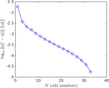
It is also informative to look at the convergence rate of from the equations with respect to growing , see Fig 3. If the error converges sufficiently fast (e.g. exponentially), then we will obtain the uniqueness of reconstruction for the case that . However, the theory about the convergence is still an open problem.

4.3 Reconstruction of only
In this numerical experiment, we are using the algorithm introduced in Section 3 to reconstruct the absorption coefficient only. We consider two scenarios for the reconstruction: (i) The datum is generated from certain model. (ii) The datum is generated from the radiative transport model. The result is summarized in the following Tab 2 and Tab 3. For all the reconstructions in the tables below, we have contaminated the datum with multiplicative random noises pointwisely by with parameter regarded as the noise level and random is the uniform distributed random variable on .
| 2.89% | 3.13% | 3.15% | 3.14% | 3.14% | 3.14% | 3.14% | 3.14% | 3.14% | |
| 3.08% | 2.88% | 2.88% | 2.89% | 2.89% | 2.89% | 2.89% | 2.89% | 2.89% | |
| 3.13% | 2.91% | 2.91% | 2.91% | 2.91% | 2.91% | 2.91% | 2.91% | 2.91% | |
| 3.09% | 2.89% | 2.88% | 2.88% | 2.88% | 2.88% | 2.88% | 2.88% | 2.88% | |
| 3.06% | 2.86% | 2.86% | 2.86% | 2.86% | 2.86% | 2.86% | 2.86% | 2.86% | |
| 3.07% | 2.88% | 2.88% | 2.88% | 2.88% | 2.88% | 2.88% | 2.88% | 2.88% | |
| 3.11% | 2.91% | 2.91% | 2.91% | 2.91% | 2.91% | 2.91% | 2.91% | 2.91% | |
| 3.09% | 2.88% | 2.88% | 2.88% | 2.88% | 2.88% | 2.88% | 2.88% | 2.88% | |
| 3.10% | 2.89% | 2.89% | 2.89% | 2.89% | 2.89% | 2.89% | 2.89% | 2.89% | |
| 3.58% | 3.14% | 3.16% | 3.18% | 3.19% | 3.19% | 3.19% | 3.19% | 3.20% |
| 2.91% | 3.17% | 3.22% | 3.22% | 3.22% | 3.22% | 3.22% | 3.22% | 3.22% | |
| 3.10% | 2.88% | 2.89% | 2.90% | 2.90% | 2.90% | 2.90% | 2.90% | 2.90% | |
| 3.14% | 2.89% | 2.89% | 2.89% | 2.89% | 2.89% | 2.89% | 2.89% | 2.89% | |
| 3.15% | 2.89% | 2.88% | 2.88% | 2.88% | 2.88% | 2.89% | 2.89% | 2.89% | |
| 3.16% | 2.91% | 2.89% | 2.89% | 2.89% | 2.89% | 2.89% | 2.89% | 2.89% | |
| 3.14% | 2.89% | 2.87% | 2.87% | 2.87% | 2.87% | 2.87% | 2.87% | 2.87% | |
| 3.12% | 2.88% | 2.87% | 2.87% | 2.87% | 2.87% | 2.87% | 2.87% | 2.87% | |
| 3.17% | 2.91% | 2.90% | 2.89% | 2.89% | 2.89% | 2.89% | 2.89% | 2.89% | |
| 3.16% | 2.90% | 2.89% | 2.89% | 2.89% | 2.89% | 2.89% | 2.89% | 2.89% | |
| 8.02% | 7.12% | 6.77% | 6.65% | 6.60% | 6.59% | 6.60% | 6.60% | 6.61% |
Observe the diagonals of above tables, one can find out that the reconstruction error is not growing as grows, this is because the estimate in Theorem 3.1 is only meant for the worst boundary source. For the given source function and coefficient set, the reconstruction based on model (diffusion approximation) appears not as good as the other models when the data are generated from models. While the performances of most low order models () are already close to the ones of high order models ().
Particularly, when the datum is generated from the radiative transport model, all of the reconstruction errors of models become larger due to the additional modeling errors, see Section 4.2. We plot some of the reconstructions in Fig 4. It is not surprising to find that the errors are relatively larger near boundary since the equation system is still elliptic over the whole domain, while the behavior of radiative transport averaged solution is hyperbolic in the vicinity of boundary sets.


4.4 Reconstruction of only
The reconstruction of is a nonlinear problem for . In order to provide a fair comparison of across the models, we will use the optimization based method to reconstruct the scattering coefficient:
| (84) |
where is the measured datum and is the regularization parameter. The optimization problem is solved by L-BFGS method, the gradient is computed from the adjoint state technique. The choice of regularization parameter should depend on the noise level. One should notice that we use norm instead of the traditional minimization:
| (85) |
This is due to the stability estimate in Theorem 3.7, where actually the norm is needed for the stability estimate. However, such regularity requirement implies that needs to be globally from Sobolev embedding, which means our finite element space needs to equip with polynomials of five or higher degrees (e.g. Argyris element). Here we relax objective functional to norm simply to avoid the extraordinary computational cost. To get a brief impression about the two optimization schemes, we take the source function with model (both data generation and reconstruction) for an example, the datum is not contaminated (noise level ) and regularization parameter as well. The reconstructed scattering coefficients are shown in Fig 5. One can tell from the images that the coefficient recovered from optimization (85) still contains background artifacts. The reason behind is the relatively strong smoothing effect of the mapping , where the high frequency information in could not be fully recovered if we emphasize equally on ’s frequency information.


Therefore the data contamination should be treated carefully for the minimization (84). This is because if we still apply the random noises by at each mesh node, then , where is the total number of nodes assuming the mesh is uniform. Therefore instead of pointwise multiplicative noise, we aggressively contaminate the datum by perturbing its Fourier modes
| (86) |
where we have used as the noise level parameter. Note that such noise will perturb the low frequency modes of which might cause severe global artifacts in the reconstruction.
| 12.0% | 19.0% | 19.5% | 19.6% | 19.6% | 19.6% | 19.6% | 19.7% | 19.7% | |
| 13.9% | 12.1% | 12.5% | 12.8% | 13.0% | 13.2% | 13.3% | 13.4% | 13.5% | |
| 14.9% | 12.5% | 12.3% | 12.5% | 12.7% | 12.9% | 13.0% | 13.1% | 13.2% | |
| 15.1% | 13.3% | 12.5% | 12.1% | 11.9% | 11.8% | 11.7% | 11.7% | 11.6% | |
| 15.1% | 13.3% | 12.5% | 12.3% | 12.2% | 12.3% | 12.3% | 12.4% | 12.4% | |
| 15.5% | 14.4% | 13.3% | 12.7% | 12.3% | 12.0% | 11.8% | 11.7% | 11.6% | |
| 15.1% | 13.8% | 12.8% | 12.5% | 12.3% | 12.2% | 12.2% | 12.2% | 12.2% | |
| 15.7% | 15.1% | 14.0% | 13.2% | 12.7% | 12.3% | 12.1% | 12.0% | 11.8% | |
| 15.2% | 14.2% | 13.1% | 12.7% | 12.4% | 12.3% | 12.2% | 12.2% | 12.2% | |
| 25.8% | 25.7% | 18.3% | 21.5% | 36.9% | 37.2% | 39.2% | 39.3% | 39.4% |
| 20.8% | 21.4% | 21.3% | 23.1% | 21.4% | 21.4% | 21.5% | 21.6% | 21.7% | |
| 23.1% | 18.0% | 18.6% | 19.1% | 19.7% | 19.9% | 20.2% | 20.3% | 20.5% | |
| 26.9% | 18.3% | 17.7% | 18.0% | 18.3% | 18.5% | 18.6% | 18.6% | 18.7% | |
| 28.0% | 22.7% | 18.2% | 16.4% | 16.3% | 16.4% | 16.6% | 16.8% | 16.9% | |
| 29.0% | 19.9% | 18.0% | 17.8% | 17.7% | 17.8% | 17.9% | 18.06% | 18.1% | |
| 29.4% | 19.5% | 16.9% | 16.4% | 16.3% | 16.3% | 16.4% | 16.4% | 16.5% | |
| 29.5% | 21.0% | 18.4% | 18.0% | 17.8% | 17.8% | 17.8% | 17.8% | 17.9% | |
| 30.2% | 20.6% | 17.3% | 16.6% | 16.4% | 16.3% | 16.3% | 16.3% | 16.4% | |
| 30.5% | 21.5% | 19.4% | 18.1% | 17.9% | 17.8% | 17.7% | 17.8% | 17.8% | |
| 55.9% | 47.8% | 49.4% | 50.2% | 50.3% | 50.3% | 51.4% | 51.5% | 51.6% |
Similar to the previous numerical experiment, we summarize the result in the Tab 4, where we have fixed the regularization parameter for these experiments. From the table, we could clearly see that is not as good as other models for the reconstruction of when the datum is coming from higher order models.
The reconstruction errors on the diagonal of the tables look converging as the order grows, which indicates that the models converge relatively fast for the given source functions and the coefficient setting. When the datum is generated from the radiative transport equation, the reconstruction error becomes larger. The reconstructions with respect to source function are significantly worse than the ones for , see Fig 6. However, this could be explained through the analogue with the model, where the scattering coefficient’s reconstruction is to solve a transport equation [5]:
| (87) |
where , where and are known. Therefore when , the function could be solved by tracing the characteristics. If vanishes or appears to be small, then the characteristics could be trapped, where the reconstructions are based on regularization only.


4.5 Reconstruction of and
In this section, we consider the non-linearized case and follow the aforementioned two-step reconstruction strategy. Suppose are the data sets measured with boundary source functions and , respectively. Our numerical reconstruction solves the optimization problem:
| (88) |
where are the solutions to the equation with the absorption coefficient and source function , respectively. Intuitively, the ratio should be quite smooth and weakly depends on , which means the reconstruction for could be very unstable. In the following, we assume the data sets and are generated from the models with multiplicative noise for only, the regularization parameter is fixed as . Then we reconstruct the absorption coefficient using the same model. The reconstructions are shown in Fig 7, it could be seen that the reconstructions are very unstable even for small noise, only limited resolution could be obtained.


4.6 Reconstruction of and
Similar to the previous case, we consider the reconstruction in a two-step process as well. Suppose are the data sets with boundary sources , respectively. Our algorithm will first construct the scattering coefficient from the following optimization problem:
| (89) |
where are the solutions to the modified equation (21), where has been replaced by , . Here we have taken the minimization. In the following numerical experiment, we assume are generated from the model, the data sets are contaminated on the Fourier space through
with . We also fix the regularization parameter .The numerical reconstructions are performed over the same model and the results are illustrated in Fig 8. After the scattering coefficient has been reconstructed, we will use the recovered scattering coefficient to find the absorption coefficient following the Experiment 4.4. The corresponding reconstruction errors of the absorption coefficients are shown in Fig 9. It can be seen that even the reconstruction of scattering coefficients contain background artifacts, while the reconstruction errors of are still quite small.


5 Conclusion
In this work, we studied the quantitative photoacoustic tomography with the simplified approximation model to the radiative transport equation. We have derived the uniqueness and stability estimates for the reconstruction of one single coefficient of , , ) from one initial pressure datum . For the simultaneous reconstruction of two coefficients, we have considered the linearized setting and introduced the optimization based numerical algorithm for the reconstruction. We showed the numerical simulations based on a synthetic data to validate the mathematical analysis.
Acknowledgment
H. Zhao’s research is partially supported by NSF DMS-2048877 and DMS-2012860.
Appendix A Appendix
Lemma A.1.
Let be the -th entry of , then
| (90) |
Proof.
Let be the matrix with -th entry as , we then compute the -th entry of by . If , , therefore . If , notice that now , we must have . If , we compute directly
| (91) |
Hence . ∎
Lemma A.2.
, hence .
Proof.
Since
| (92) | ||||
which gives the factorization
| (93) |
where diagonal matrices
| (94) | ||||
with and is the Cauchy-Toeplitz matrix,
| (95) |
We denote and , then use the Theorem 2.1 in [36],
| (96) |
where and satisfy
| (97) | ||||
Also are computed explicitly by Cramer’s law,
| (98) | ||||
By replacing with their values, we obtain
| (99) | ||||
Then we can easily deduce , since all matrices involved are diagonal, let , then from the theory of Gamma functions, we know
| (100) |
Hence we can estimate ’s upper bound by estimating
| (101) | ||||
Then by noticing the Chu’s Double Inequality [7],
| (102) |
the following estimates hold,
| (103) | ||||
which implies
| (104) | ||||
∎
Lemma A.3.
.
Proof.
We show that for all ,
| (105) |
The above estimate is true for since , we only focus on the cases that . Reformulate by the Gamma function as
| (106) |
From the Chu’s Double Inequality [7]
| (107) |
the following estimates hold,
| (108) |
we can deduce the estimate
| (109) | ||||
The other part can be estimated in a similar way,
| (110) | ||||
Hence we can estimate that
| (111) |
the above estimate is strictly less than for , then the Frobenius norm’s square of is estimated by
| (112) |
∎
References
- [1] M. Agranovsky, P. Kuchment, and L. Kunyansky, On reconstruction formulas and algorithms for the thermoacoustic and photoacoustic tomography, Preprint, (2007).
- [2] H. Ammari, E. Bretin, V. Jugnon, and A. Wahab, Photoacoustic imaging for attenuating acoustic media, in Mathematical modeling in biomedical imaging II, Springer, 2012, pp. 57–84.
- [3] G. Bal, Hybrid inverse problems and internal functionals, Inverse problems and applications: inside out. II, 60 (2013), pp. 325–368.
- [4] G. Bal, A. Jollivet, and V. Jugnon, Inverse transport theory of photoacoustics, Inverse Problems, 26 (2010), p. 025011.
- [5] G. Bal and K. Ren, Multi-source quantitative photoacoustic tomography in a diffusive regime, Inverse Problems, 27 (2011), p. 075003.
- [6] P. Beard, Biomedical photoacoustic imaging, Interface focus, 1 (2011), pp. 602–631.
- [7] J. Chu, A modified wallis product and some applications, The American Mathematical Monthly, 69 (1962), pp. 402–404.
- [8] M. Chu, K. Vishwanath, A. D. Klose, and H. Dehghani, Light transport in biological tissue using three-dimensional frequency-domain simplified spherical harmonics equations, Physics in Medicine & Biology, 54 (2009), p. 2493.
- [9] B. Cox, J. Laufer, and P. Beard, The challenges for quantitative photoacoustic imaging, in Photons Plus Ultrasound: Imaging and Sensing 2009, vol. 7177, International Society for Optics and Photonics, 2009, p. 717713.
- [10] T. Ding, K. Ren, and S. Vallélian, A one-step reconstruction algorithm for quantitative photoacoustic imaging, Inverse Problems, 31 (2015), p. 095005.
- [11] Y. Fan, J. An, and L. Ying, Fast algorithms for integral formulations of steady-state radiative transfer equation, Journal of Computational Physics, 380 (2019), pp. 191–211.
- [12] C. Frederick, K. Ren, and S. Vallélian, Image reconstruction in quantitative photoacoustic tomography with the simplified p_2 approximation, SIAM Journal on Imaging Sciences, 11 (2018), pp. 2847–2876.
- [13] H. Gao and H. Zhao, Analysis of a numerical solver for radiative transport equation, Mathematics of computation, 82 (2013), pp. 153–172.
- [14] W. Gautschi, Some elementary inequalities relating to the gamma and incomplete gamma function, J. Math. Phys, 38 (1959), pp. 77–81.
- [15] E. M. Gelbard, Application of spherical harmonics method to reactor problems, Bettis Atomic Power Laboratory, West Mifflin, PA, Technical Report No. WAPD-BT-20, (1960).
- [16] A. D. Güngör, Erratum to “an upper bound for the condition number of a matrix in spectral norm”[j. comput. appl. math. 143 (2002) 141–144], Journal of Computational and Applied Mathematics, 234 (2010), p. 316.
- [17] M. Haltmeier, T. Schuster, and O. Scherzer, Filtered backprojection for thermoacoustic computed tomography in spherical geometry, Mathematical methods in the applied sciences, 28 (2005), pp. 1919–1937.
- [18] Y. Hristova, Time reversal in thermoacoustic tomography—an error estimate, Inverse Problems, 25 (2009), p. 055008.
- [19] A. D. Klose and E. W. Larsen, Light transport in biological tissue based on the simplified spherical harmonics equations, Journal of Computational Physics, 220 (2006), pp. 441–470.
- [20] , Simplified spherical harmonics methods for modeling light transport in biological tissue, in Biomedical Topical Meeting, Optical Society of America, 2006, p. MH3.
- [21] P. Kuchment and L. Kunyansky, Mathematics of thermoacoustic and photoacoustic tomography, preprint, (2007).
- [22] W. Li, Y. Yang, and Y. Zhong, Inverse transport problem in fluorescence ultrasound modulated optical tomography with angularly averaged measurements, Inverse Problems, 36 (2020), p. 025011.
- [23] A. V. Mamonov and K. Ren, Quantitative photoacoustic imaging in radiative transport regime, arXiv preprint arXiv:1207.4664, (2012).
- [24] A. W. Marshall, I. Olkin, and B. C. Arnold, Inequalities: theory of majorization and its applications, vol. 143, Springer, 1979.
- [25] R. G. McClarren, Theoretical aspects of the simplified pn equations, Transport Theory and Statistical Physics, 39 (2010), pp. 73–109.
- [26] W. McLean and W. C. H. McLean, Strongly elliptic systems and boundary integral equations, Cambridge university press, 2000.
- [27] G. Piazza and T. Politi, An upper bound for the condition number of a matrix in spectral norm, Journal of Computational and Applied Mathematics, 143 (2002), pp. 141–144.
- [28] K. Ren, H. Gao, and H. Zhao, A hybrid reconstruction method for quantitative pat, SIAM Journal on Imaging Sciences, 6 (2013), pp. 32–55.
- [29] K. Ren, R. Zhang, and Y. Zhong, Inverse transport problems in quantitative pat for molecular imaging, Inverse Problems, 31 (2015), p. 125012.
- [30] , A fast algorithm for radiative transport in isotropic media, Journal of Computational Physics, 399 (2019), p. 108958.
- [31] K. Ren and H. Zhao, Quantitative fluorescence photoacoustic tomography, SIAM Journal on Imaging Sciences, 6 (2013), pp. 2404–2429.
- [32] K. Ren, H. Zhao, and Y. Zhong, Separability of the kernel function in an integral formulation for anisotropic radiative transfer equation, arXiv preprint arXiv:1908.10467, (2019).
- [33] K. Ren and Y. Zhong, Unique determination of absorption coefficients in a semilinear transport equation, arXiv preprint arXiv:2007.09516, (2020).
- [34] O. Scherzer, Handbook of mathematical methods in imaging, Springer Science & Business Media, 2010.
- [35] P. Stefanov and G. Uhlmann, Thermoacoustic tomography with variable sound speed, Inverse Problems, 25 (2009), p. 075011.
- [36] E. E. Tyrtyshnikov, Singular values of cauchy-toeplitz matrices, Linear algebra and its applications, 161 (1992), pp. 99–116.
- [37] L. V. Wang, Photoacoustic imaging and spectroscopy, CRC press, 2017.
- [38] S. Wright, M. Schweiger, and S. Arridge, Reconstruction in optical tomography using the pn approximations, Measurement Science and Technology, 18 (2006), p. 79.
- [39] W. P. Ziemer, Weakly differentiable functions: Sobolev spaces and functions of bounded variation, vol. 120, Springer Science & Business Media, 2012.