Unbiased Subdata Selection for Fair Classification:
A Unified Framework and Scalable Algorithms

In this subsection, we present an overview of fairness measures and existing methods for fair classification.

This paper first studies fair support vector machine (SVM) as a motivating example. We formulate the generalized SVM (GSVM) model as a mixed-integer program to model exact fairness, and then study the model properties, develop scalable algorithms for solving the generalized SVM with fairness (GSVMF) as well as study the extensions to other popular classification models including deep learning with different fairness measures. Specifically, our framework can be formulated as

$\displaystyle\underset{(\bm{w},b,\bm{u})\in U,\bm{z}}{\min}$

$\displaystyle\left\{\underbrace{\mathcal{A}(\bm{z},t\bm{e}-\bm{u})}_{\text{Classification Outcome}}+\lambda\underbrace{\mathcal{R}(\bm{w},b,\bm{u})}_{\text{Regularization}}+\rho\underbrace{{\mathcal{F}}(\bm{z})}_{\text{Fairness Measure}}:\bm{z}\in Z\right\},$

(1)

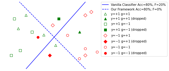
where $t\in{\mathbb{R}}$ is the prediction threshold, vector $\bm{u}$ represents classification outcomes (e.g., violation margins, prediction probabilities) under a particular classifier specified by unknown parameters $\bm{w},b$, $\mathcal{R}(\bm{w},b,\bm{u})$ denotes the regularization term for the classifier with tuning parameter $\lambda\geq 0$, binary vector $\bm{z}\in Z$ indicates the correct classification corresponding to subdata selection decisions, and binary set $Z$ denotes the domain of $\bm{z}$. The binary vector $\bm{z}$ can be used to model the statistical fairness measures precisely without any approximation. In the unified framework (1), function $\mathcal{A}(\bm{z},t\bm{e}-\bm{u})$, which is often bilinear, denotes the classification outcomes and the function ${\mathcal{F}}(\bm{z})$ denotes a fairness measure, where a Pareto optimality between accuracy and fairness is achieved by a proper penalty parameter $\rho>0$. Table 2 displays the function $\mathcal{A}(\bm{z},t\bm{e}-\bm{u})$ and function $\mathcal{R}(\bm{w},b,\bm{u})$ for well-known classifiers. Table 3 shows function ${\mathcal{F}}(\bm{z})$ for four popular fairness measures. Besides, since the optimized binary decisions $\bm{z}$ take values $\{0,1\}$ according to the tradeoff of accuracy and fairness, the proposed method has the subdata selection interpretation. That is, we will select the data points such that their $z$ values are equal to one and train the classifier only using the selected subdata. Therefore, the proposed framework can select unbiased data points for fair classification and can be naturally solved using the iterative refining strategy with two subroutines, i.e., subdata selection and classification using the selected subdata. We illustrate the subdata selection in Figure 1. Note that Figure 1(a) demonstrates the decision boundary for the vanilla classifier which may not be fair to the protected groups, while Figure 1(b) shows that the unbiased subdata selection in the proposed framework can reduce the unfairness score to 0% while achieving the same accuracy as vanilla classifier.

As illustrated in Figure 2, the main contributions of this paper are summarized below:

1. (i)

   We propose a generalized SVM (GSVM) model for the binary classification problems and prove that it is Fisher consistent. We incorporate the overall misclassification rate (OMR) precisely in the generalized SVM model, termed “GSVMF”;

2. (ii)

   We propose an exact mixed-integer conic programming formulation for GSVMF, which can be solved by off-the-shelf solvers for the moderate-sized instances;

3. (iii)

   For the large-scale instances, we propose to solve GSVMF effectively to near-optimality using the iterative refining strategy (IRS) by employing an unbiased subdata selection when fixing the classification outcomes and executing a classifier given the selected subdata in an alternative fashion. In the proposed IRS, the subdata selection, albeit resorting to a binary program, is strongly polynomial-solvable with time complexity of $O(N\log{N})$, where $N$ denotes the number of data points. We also study the convergence property of IRS and derive its approximation bound;

4. (iv)

   We show that the proposed GSVMF is also amenable to represent other fairness measures such as false positive rate, equal opportunity, and demographic parity; and

5. (v)

   We further present the extensions to fair multiclass classification, logistic regression with fairness, kernel SVM with fairness, fair deep learning, and classification with unbalanced data.

The remainder of this paper is organized as follows. Section 2 presents the model formulation and model properties of GSVMF. Section 3 studies the unbiased subdata selection method and the iterative refining strategy for solving GSVMF. Section 4 and Section 5 demonstrate the extensions to other fairness measures and different classifiers, respectively. Section 6 presents the application to classification with unbalanced data. Section 7 shows the numerical experiments. Section 8 concludes the paper.

Note that in SVM (2), for each data point $i\in[N]$, the violation margin $u_{i}$ helps predict the classification results, i.e., if $u_{i}$ is less than or equal to some threshold, then we predict $i$th data point to be of the same label as $y_{i}$, and misclassify it, otherwise. Thus, this observation inspires us to improve SVM using an indicator function $\mathbbm{1}\left(u_{i}\leq t\right)$ to minimize the sum of misclassification margins, where t is the threshold. Specifically, we propose the following generalized SVM (GSVM)

$$v:=\underset{\bm{w},b,\bm{u}}{\min}\left\{\frac{1}{N}\sum_{i\in[N]}(u_{i}-t)\mathbbm{1}\left(u_{i}\leq t\right)+\lambda\|\bm{w}\|^{2}_{2}:y_{i}(\bm{x}^{\top}_{i}\bm{w}+b)\geq 1-u_{i},u_{i}\geq 0,\forall{i\in{[N]}}\right\},$$

(3)

We remark that (i) if $t\rightarrow+\infty$, GSVM (3) becomes SVM (2); (ii) one can choose $t$ properly through cross-validation; and (iii) although being intractable, GSVM (3) can be useful to incorporate many fairness measures and we will show later that it can be solved effectively via an off-the-shelf solver for moderate-sized instances and an iterative refining strategy for large-scale instances.

Next, we observe that in GSVM (3), for each $i\in[N]$, the indicator function $\mathbbm{1}\left(u_{i}\leq t\right)$ can be replaced by the binary variable $z_{i}$, where $z_{i}=1$ indicates correct classification and $z_{i}=0$ indicates misclassification with respect to the threshold $t$. We see that, GSVM (3) admits an equivalent mixed-integer biconvex programming formulation.

The binary variables $\bm{z}$ enable us to distinguish the correct classified and misclassified data points. Thus, we can model the fairness using these binary variables. Note that the biconvex program (4) can be equivalently reformulated as a mixed-integer conic program (MICP) with the following McCormick inequalities to linearize the bilinear terms $\{z_{i}u_{i}\}_{i\in[N]}$

$$s_{i}\leq M_{u}z_{i},\quad s_{i}\leq u_{i},\quad s_{i}\geq 0,\quad s_{i}\geq u_{i}-M_{u}(1-z_{i}),\forall i\in[N]$$

(5)

where $M_{u}$ is a positive large number and its derivation will be postponed to the next proposition. The result of MICP is summarized below.

This result allows us to use off-the-shelf solvers such as Gurobi and CPLEX to solve (6) to optimality when the number of data points is not very large, and we can also use the optimal solution from this exact formulation to test the effectiveness of the proposed iterative refining strategy.

The next proposition shows how to compute the big-M coefficient $M_{u}$ from GSVM (6) in closed-form. The proof idea is to (i) use the optimality condition; and (ii) discuss different cases of label $y_{i}$ for each $i\in[N]$.

In this subsection, we prove Fisher consistency of the proposed GSVM (4), which further demonstrates the correctness of the proposed model. Given a realization $\bm{x}$ of random observation $\tilde{\bm{x}}$, let us define

$$p(\bm{x})={\mathbb{P}}\left\{\tilde{y}=1\mid\tilde{\bm{x}}=\bm{x}\right\},$$

i.e., $p(\bm{x})$ defines the probability that the label of data $\bm{x}$ equals to $1$. Following Lee et al. 2004; Lin 2002; Liu 2007, we consider the Bayesian decision rule $\phi_{B}(\bm{x})$, which admits the following form

$\displaystyle\phi_{B}(\bm{x})=\begin{cases}1,\text{\rm if }p(\bm{x})\geq 0.5,\\ -1,\text{\rm if }p(\bm{x})<0.5,\end{cases}$

(7)

i.e., we assign a label for the realization $\bm{x}$ according to whether the probability $p(\bm{x})$ is greater than 0.5 or not. In formulation (4), we will use a more general classifier $f(\bm{x})$ instead of the linear one $\bm{x}^{\top}\bm{w}+b$. Conditioning on the realization $\tilde{\bm{x}}=\bm{x}$ in formulation (4), we are trying to find a separator $f(\bm{x})$ to minimize the conditional expected surrogate loss. Given a realization $\bm{x}$ of the random data, we suppose that the classifier $f(\bm{x})$ is normalized to be between $-t-1$ and $t+1$. The classification problem is equivalent to

$\displaystyle\min_{f(\bm{x}),\tilde{u}}\left\{{\mathbb{E}}[(\tilde{u}-t)\mathbbm{1}\left(\tilde{u}\leq t\right)|\tilde{\bm{x}}=\bm{x}]:\tilde{y}f(\tilde{\bm{x}})\geq 1-\tilde{u},\tilde{u}\geq 0,-t-1\leq f(\bm{x})\leq t+1\right\}.$

(8)

Projecting out random variable $\tilde{u}$, formulation (8) is equivalent to

	$\displaystyle\min_{f(\bm{x})}$	$\displaystyle\left\{L(f(\bm{x})):={\mathbb{E}}_{\tilde{y}}\left[\max\{-\tilde{y}f(\tilde{\bm{x}})+1-t,-t\}\mathbbm{1}(\tilde{y}f(\tilde{\bm{x}})\geq t-1)|\tilde{\bm{x}}=\bm{x}\right]:\right.$		(9)
		$\displaystyle\left.-t-1\leq f(\bm{x})\leq t+1\right\}.$

Thus, the expected loss minimization problem can be formally defined as

$\displaystyle f^{*}(\bm{x})\in\arg\min_{f(\bm{x})}\left\{L(f(\bm{x})):-t-1\leq f(\bm{x})\leq t+1\right\},$

(10)

where we let $f^{*}(\bm{x})$ denote an optimal classifier.

Next, following the spirit of seminal works (Lee et al. 2004; Lin 2002; Liu 2007), we make a formal definition of Fisher consistency for the binary classification problem.

Now we are ready to show the consistency of the loss function $L(\bm{f}(\bm{x}))$.

Proposition 5 shows that similar to SVM (Lin 2002), GSVM (4) is also Fisher consistent. This demonstrates that the performance of the proposed GSVM (4) is at least as good as SVM for the binary classification problems. We remark that the similar Fisher consistency result holds for the multi-class SVM.

In this subsection, we will illustrate the modeling power of GSVM (4) by augmenting it with one popular fairness measure, overall misclassification rate (OMR). Extensions to other fairness measures can be found in Section 4.

The OMR (see, e.g., Zafar et al. 2019) fairness accounts for the misclassification measure of disparate mistreatment. The classifier has no disparate mistreatment if different groups have the same misclassification rates. Suppose that there is a protected feature corresponding to two groups denoted by $g\in\{-1,1\}$. Then OMR fairness measure can be defined as below.

The fairness measure function $F_{\rm OMR}$ is the absolute difference of the misclassification rates of both groups. We then use the binary variables $\bm{z}$ to exactly represent the OMR fairness measure

	$\displaystyle F_{\rm OMR}$	$\displaystyle=\left|{\mathbb{P}}(\tilde{u}\leq t|\tilde{g}=+1)-{\mathbb{P}}(\tilde{u}\leq t|\tilde{g}=-1)\right|=\left|\sum_{i\in{\mathcal{D}}_{+}}\frac{z_{i}}{D_{+}}-\sum_{i\in{\mathcal{D}}_{-}}\frac{z_{i}}{D_{-}}\right|,$		(11a)
where two sets
	$${\mathcal{D}}_{+}=\{i\in[N]:g_{i}=+1\},{\mathcal{D}}_{-}=\{i\in[N]:g_{i}=-1\}$$			(11b)

represent index subsets of data points from each protected group, respectively, and $D_{+}=|{\mathcal{D}}_{+}|$ is the number of group $g=+1$ data points, and $D_{-}=|{\mathcal{D}}_{-}|$ is the number of group $g=-1$ data points.

To prevent discrimination in prediction, we penalize the unfairness in our proposed GSVM (4) with nonnegative penalty $\rho$. Therefore, we formulate the following GSVMF model

$$v_{\rho}:=\underset{\bm{w},b,\bm{u},\bm{z}}{\min}\left\{\underbrace{\frac{1}{N}\sum_{i\in[N]}z_{i}(u_{i}-t)}_{\mathcal{A}(\bm{z},t\bm{e}-\bm{u})}+\lambda\underbrace{\|\bm{w}\|^{2}_{2}}_{\mathcal{R}(\bm{w},b,\bm{u})}+\rho\underbrace{\left|\sum_{i\in{\mathcal{D}}_{+}}\frac{z_{i}}{D_{+}}-\sum_{i\in{\mathcal{D}}_{-}}\frac{z_{i}}{D_{-}}\right|}_{{\mathcal{F}}(\bm{z})}:\eqref{eq_plane}-\eqref{eq_binary_z}\right\}$$

(12)

where $\rho$ is the penalty factor that balances the prediction accuracy and fairness. Clearly, the proposed GSVMF (12) is a special case of the framework (1). Note that GSVMF (12) has non-convex terms $\{z_{i}u_{i}\}_{i\in[N]}$. We can linearize them using McCormick inequalities (5). Thus, similar to Proposition 2, GSVMF (12) can be formulated as a MICP.

We remark that for the moderate-sized instances, one might be able to solve both MICPs easily via off-the-shelf solvers such as Gurobi and CPLEX.

The observation that GSVMF (12) is a special case of the framework (1) leads to the following remarks.

1. (i)

   The binary variables $\bm{z}$ indicate the subdata selection decisions. Data points with their corresponding $z-$variables taking value of 1 are the potential unbiased ones selected by the model, and the other data points are ignored. This gives rise to an iterative refining strategy described in Section 3 that improves the subdata selection decisions $\bm{z}$ and classification accuracy in an alternating way;

2. (ii)

   The proposed GSVMF (12) can be quite flexible. Indeed, if we replace $u_{i}$ by the probabilities of classification outcomes and let $t$ denote the misclassification threshold, then GSVMF (12) can be generalized to other classification models with fairness including logistic regression and convolutional neural networks (CNNs). These facts will be elaborated in the subsequent sections;

3. (iii)

   Since the classification results are discrete (e.g., $\{0,1\}$ for the binary classification), it is natural to model the fairness measures using discrete variables, for which GSVMF (12) paves a generic way;

4. (iv)

   For the moderate-sized datasets, we can use exact approaches to solve GSVMF (12) to optimality. For the large-scale optimization, we propose to use the iterative refining strategy (see Section 3), which works extremely well in our numerical study;

5. (v)

   If one would like to add the OMR fairness measure as a constraint, the similar results still hold; and

6. (vi)

   The OMR fairness measure in GSVMF (12) can be replaced by other fairness measures such as false positive rate (FPR), equal opportunity, and demographic parity, which will be elaborated in Section 4.

We observe that the absolute term in the objective function in GSVMF (12) can be split into two parts by discussing its sign, and therefore GSVMF (12) can be computed by solving two distinct optimization problems. This observation will be particularly important when we design the iterative refining strategy for solving GSVMF (12) in Section 3.

	$\displaystyle v_{\rho 1}:=\underset{\bm{w},b,\bm{u},\bm{z}}{\text{min}}$	$\displaystyle\frac{1}{N}\sum_{i\in[N]}z_{i}(u_{i}-t)+\lambda\|\bm{w}\|^{2}_{2}-\rho\sum_{i\in{\mathcal{D}}_{+}}\frac{z_{i}}{D_{+}}+\rho\sum_{i\in{\mathcal{D}}_{-}}\frac{z_{i}}{D_{-}},$		(13a)
	$\displaystyle\text{\rm(GSVMF-1)}\quad\text{s.t.}$	$\displaystyle\sum_{i\in{\mathcal{D}}_{+}}D_{-}z_{i}-\sum_{i\in{\mathcal{D}}_{-}}D_{+}z_{i}\leq 0,$
		$\displaystyle\eqref{eq_plane}-\eqref{eq_binary_z};\$
	$\displaystyle v_{\rho 2}:=\underset{\bm{w},b,\bm{u},\bm{z}}{\text{min}}$	$\displaystyle\frac{1}{N}\sum_{i\in[N]}z_{i}(u_{i}-t)+\lambda\|\bm{w}\|^{2}_{2}+\rho\sum_{i\in{\mathcal{D}}_{+}}\frac{z_{i}}{D_{+}}-\rho\sum_{i\in{\mathcal{D}}_{-}}\frac{z_{i}}{D_{-}},$		(13b)
	$\displaystyle\text{\rm(GSVMF-2)}\quad\text{s.t.}$	$\displaystyle\sum_{i\in{\mathcal{D}}_{+}}D_{-}z_{i}-\sum_{i\in{\mathcal{D}}_{-}}D_{+}z_{i}\geq 0,$
		$\displaystyle\eqref{eq_plane}-\eqref{eq_binary_z}.$

In this subsection, we observe that if $\rho$ is large enough or more precisely, if there exists a threshold $\bar{\rho}$ such that $\rho\geq\bar{\rho}$, then the fairness measure becomes zero and GSVMF (12) becomes the following GSVMF0

$$\underset{\bm{w},b,\bm{u},\bm{z}}{\min}\left\{\frac{1}{N}\sum_{i\in[N]}z_{i}(u_{i}-t)+\lambda\|\bm{w}\|^{2}_{2}:\left|\sum_{i\in{\mathcal{D}}_{+}}\frac{z_{i}}{D_{+}}-\sum_{i\in{\mathcal{D}}_{-}}\frac{z_{i}}{D_{-}}\right|=0,\eqref{eq_plane}-\eqref{eq_binary_z}\right\},$$

(14)

i.e., zero-tolerance GSVMF (12). This result is summarized below.

Since $(\bm{w}^{*},b^{*},\bm{u}^{*},\bm{z}^{*})$ is feasible to GSVMF (12), thus we have $v^{*}\geq\widehat{v}_{\rho}$. Thus, it remains to show that $v^{*}\leq\widehat{v}_{\rho}$ when $\rho\geq\bar{\rho}$, $\bar{\rho}>0$. We prove it by contradiction. Suppose $v^{*}>\widehat{v}_{\rho}$, which implies that $(\bm{w}^{*},b^{*},\bm{u}^{*},\bm{z}^{*})$ is not optimal to GSVMF (12), or equivalently, $(\widehat{\bm{w}},\widehat{b},\widehat{\bm{u}},\widehat{\bm{z}})$ is not optimal to GSVMF0 (14). Hence, due to optimality condition, we must have

$\displaystyle\left|\sum_{i\in{\mathcal{D}}_{+}}\frac{\widehat{z}_{i}}{D_{+}}-\sum_{i\in{\mathcal{D}}_{-}}\frac{\widehat{z}_{i}}{D_{-}}\right|>0.$

(15a)

Additionally,

		$\displaystyle\frac{1}{N}\sum_{i\in[N]}\widehat{z}_{i}(\widehat{u}_{i}-t)+\lambda\|\widehat{\bm{w}}\|^{2}_{2}=\widehat{v}_{\rho}-\rho\left|\sum_{i\in{\mathcal{D}}_{+}}\frac{\widehat{z}_{i}}{D_{+}}-\sum_{i\in{\mathcal{D}}_{-}}\frac{\widehat{z}_{i}}{D_{-}}\right|$		(15b)
		$\displaystyle<v^{*}-\rho\left|\sum_{i\in{\mathcal{D}}_{+}}\frac{\widehat{z}_{i}}{D_{+}}-\sum_{i\in{\mathcal{D}}_{-}}\frac{\widehat{z}_{i}}{D_{-}}\right|<v^{*}:=\frac{1}{N}\sum_{i\in[N]}z^{*}_{i}(u^{*}_{i}-t)+\lambda\|\bm{w}^{*}\|^{2}_{2},$

where the first inequality is due to our assumption and the second one is because of (15a).

Then according to (15a) and (15b) as well as the definition of $\widehat{s}$ and $\widehat{r}$, we must have $\widehat{s}$, $\widehat{r}>0$. Hence, we can further conclude that

$$\widehat{s}\leq\left|\sum_{i\in{\mathcal{D}}_{+}}\frac{\widehat{z}_{i}}{D_{+}}-\sum_{i\in{\mathcal{D}}_{-}}\frac{\widehat{z}_{i}}{D_{-}}\right|,$$

(15c)

	$\displaystyle\frac{1}{N}\sum_{i\in[N]}\widehat{z}_{i}(\widehat{u}_{i}-t)+\lambda\|\widehat{\bm{w}}\|^{2}_{2}$	$\displaystyle\geq\min_{\bm{w},b,\bm{u}}\left\{\frac{1}{N}\sum_{i\in[N]}\widehat{z}_{i}(u_{i}-t)+\lambda\|\bm{w}\|^{2}_{2}:\eqref{eq_plane}-\eqref{eq_binary_z}\right\}$		(15d)
		$\displaystyle\geq\frac{1}{N}\sum_{i\in[N]}z^{*}_{i}(u^{*}_{i}-t)+\lambda\|\bm{w}^{*}\|^{2}_{2}-{\widehat{r}}.$

According to (15c) and (15d), we obtain

	$\displaystyle\widehat{v}_{\rho}$	$\displaystyle=\frac{1}{N}\sum_{i\in[N]}\widehat{z}_{i}(\widehat{u}_{i}-t)+\lambda\|\widehat{\bm{w}}\|^{2}_{2}+\rho\left|\sum_{i\in{\mathcal{D}}_{+}}\frac{\widehat{z}_{i}}{D_{+}}-\sum_{i\in{\mathcal{D}}_{-}}\frac{\widehat{z}_{i}}{D_{-}}\right|$
		$\displaystyle\geq\frac{1}{N}\sum_{i\in[N]}z^{*}_{i}(u^{*}_{i}-t)+\lambda\|\bm{w}^{*}\|^{2}_{2}-{\widehat{r}}+\rho\widehat{s}.$

Thus, for $\rho\geq\bar{\rho}:=\frac{{\widehat{r}}}{\widehat{s}}$, we must have $\widehat{v}_{\rho}\geq v^{*}$, a contradiction.  

We remark that (i) the proof of Proposition 9 highly relies on the discrete nature of variables $\bm{z}$, particularly, the reason that two constants $\widehat{r}>0$ and $\widehat{s}>0$ are well defined is because binary variables $\bm{z}$ can only take a finite number of values; and (ii) the result in Proposition 9 shows that by choosing a large but finite penalty $\rho$ instead of being infinite, we are able to convert GSVMF (12) into fairness constrained GSVMF formulation.

In this subsection, we will develop a polynomial-time Algorithm 1 with running time complexity $O(N\log N)$ for solving GSVMF (12) by fixing the values of the continuous variables $(\bm{w},b,\bm{u})$. The algorithm takes advantage of the notable result in Proposition 8, that is, we can decompose the problem into two subproblems, GSVMF-1 (13a) and GSVMF-2 (13b). For each subproblem, we observe that if the total number of the correct classification outcomes of the group $g=+1$ is known, i.e., $\sum_{i\in{\mathcal{D}}_{+}}z_{i}=\textrm{\rm constant}$, then the resulting binary optimization problem can be solved effectively by sorting the objective coefficients. The formal derivation can be found below.

References

- xra (2017) NIH Chest X-rays. https://www.kaggle.com/nih-chest-xrays/data?select=Data_Entry_2017.csv, 2017.
- Abolghasemi et al. (2012) Vahid Abolghasemi, Saideh Ferdowsi, and Saeid Sanei. A gradient-based alternating minimization approach for optimization of the measurement matrix in compressive sensing. Signal Processing, 92(4):999–1009, 2012.
- Agarwal et al. (2018) Alekh Agarwal, Alina Beygelzimer, Miroslav Dudík, John Langford, and Hanna Wallach. A reductions approach to fair classification. arXiv preprint arXiv:1803.02453, 2018.
- Aghaei et al. (2019) Sina Aghaei, Mohammad Javad Azizi, and Phebe Vayanos. Learning optimal and fair decision trees for non-discriminative decision-making. In Proceedings of the AAAI Conference on Artificial Intelligence, volume 33, pages 1418–1426, 2019.
- Ayalew and Yamagishi (2005) Lulseged Ayalew and Hiromitsu Yamagishi. The application of gis-based logistic regression for landslide susceptibility mapping in the kakuda-yahiko mountains, central japan. Geomorphology, 65(1-2):15–31, 2005.
- Balashankar et al. (2019) Ananth Balashankar, Alyssa Lees, Chris Welty, and Lakshminarayanan Subramanian. What is fair? exploring pareto-efficiency for fairness constrained classifiers. arXiv preprint arXiv:1910.14120, 2019.
- Calmon et al. (2017) Flavio Calmon, Dennis Wei, Bhanukiran Vinzamuri, Karthikeyan Natesan Ramamurthy, and Kush R Varshney. Optimized pre-processing for discrimination prevention. In Advances in Neural Information Processing Systems, pages 3992–4001, 2017.
- Chen and Xie (2020) Shutong Chen and Weijun Xie. On the cluster-aware supervised learning (clusl): Frameworks, convergent algorithms, and applications. INFORMS Journal On Computing. Accepted, 2020.
- Cheng et al. (2019) Jingchun Cheng, Yali Li, Jilong Wang, Le Yu, and Shengjin Wang. Exploiting effective facial patches for robust gender recognition. Tsinghua Science and Technology, 24(3):333–345, 2019.
- Dal Pozzolo et al. (2014) Andrea Dal Pozzolo, Olivier Caelen, Yann-Ael Le Borgne, Serge Waterschoot, and Gianluca Bontempi. Learned lessons in credit card fraud detection from a practitioner perspective. Expert systems with applications, 41(10):4915–4928, 2014.
- De Bruijne (2016) Marleen De Bruijne. Machine learning approaches in medical image analysis: From detection to diagnosis, 2016.
- Donini et al. (2018) Michele Donini, Luca Oneto, Shai Ben-David, John S Shawe-Taylor, and Massimiliano Pontil. Empirical risk minimization under fairness constraints. In Advances in Neural Information Processing Systems, pages 2791–2801, 2018.
- Dreiseitl and Ohno-Machado (2002) Stephan Dreiseitl and Lucila Ohno-Machado. Logistic regression and artificial neural network classification models: a methodology review. Journal of biomedical informatics, 35(5-6):352–359, 2002.
- Du et al. (2020) Mengnan Du, Fan Yang, Na Zou, and Xia Hu. Fairness in deep learning: A computational perspective. IEEE Intelligent Systems, 2020.
- Dua and Graff (2017) Dheeru Dua and Casey Graff. UCI machine learning repository. http://archive.ics.uci.edu/ml, 2017.
- Fish et al. (2016) Benjamin Fish, Jeremy Kun, and Ádám D Lelkes. A confidence-based approach for balancing fairness and accuracy. In Proceedings of the 2016 SIAM International Conference on Data Mining, pages 144–152. SIAM, 2016.
- Goel et al. (2018) Naman Goel, Mohammad Yaghini, and Boi Faltings. Non-discriminatory machine learning through convex fairness criteria. In Thirty-Second AAAI Conference on Artificial Intelligence, 2018.
- Hajian and Domingo-Ferrer (2012) Sara Hajian and Josep Domingo-Ferrer. A methodology for direct and indirect discrimination prevention in data mining. IEEE transactions on knowledge and data engineering, 25(7):1445–1459, 2012.
- Han et al. (2012) Shunjie Han, Cao Qubo, and Han Meng. Parameter selection in svm with rbf kernel function. In World Automation Congress 2012, pages 1–4. IEEE, 2012.
- Hardt et al. (2016) Moritz Hardt, Eric Price, and Nati Srebro. Equality of opportunity in supervised learning. In Advances in neural information processing systems, pages 3315–3323, 2016.
- Jain et al. (2013) Prateek Jain, Praneeth Netrapalli, and Sujay Sanghavi. Low-rank matrix completion using alternating minimization. In Proceedings of the forty-fifth annual ACM symposium on Theory of computing, pages 665–674, 2013.
- (22) Lauren Kirchner Jeff Larson, Surya Mattu and Julia Angwin. How we analyzed the compas recidivism algorithm. https://www.propublica.org/article/how-we-analyzed-the-compas-recidivism-algorithm.
- Jeni et al. (2013) László A Jeni, Jeffrey F Cohn, and Fernando De La Torre. Facing imbalanced data–recommendations for the use of performance metrics. In 2013 Humaine association conference on affective computing and intelligent interaction, pages 245–251. IEEE, 2013.
- Kamiran and Calders (2012) Faisal Kamiran and Toon Calders. Data preprocessing techniques for classification without discrimination. Knowledge and Information Systems, 33(1):1–33, 2012.
- Kamishima et al. (2012) Toshihiro Kamishima, Shotaro Akaho, Hideki Asoh, and Jun Sakuma. Fairness-aware classifier with prejudice remover regularizer. In Joint European Conference on Machine Learning and Knowledge Discovery in Databases, pages 35–50. Springer, 2012.
- Kilbertus et al. (2017) Niki Kilbertus, Mateo Rojas Carulla, Giambattista Parascandolo, Moritz Hardt, Dominik Janzing, and Bernhard Schölkopf. Avoiding discrimination through causal reasoning. In Advances in Neural Information Processing Systems, pages 656–666, 2017.
- Lai and Varghese (2017) Ming Jun Lai and Abraham Varghese. On convergence of the alternating projection method for matrix completion and sparse recovery problems. arXiv preprint arXiv:1711.02151, 2017.
- Lee et al. (2004) Yoonkyung Lee, Yi Lin, and Grace Wahba. Multicategory support vector machines: Theory and application to the classification of microarray data and satellite radiance data. Journal of the American Statistical Association, 99(465):67–81, 2004.
- Liao et al. (2014) Xuejun Liao, Hui Li, and Lawrence Carin. Generalized alternating projection for weighted-2,1 minimization with applications to model-based compressive sensing. SIAM Journal on Imaging Sciences, 7(2):797–823, 2014.
- Lin (2002) Yi Lin. Support vector machines and the bayes rule in classification. Data Mining and Knowledge Discovery, 6(3):259–275, 2002.
- Liu (2007) Yufeng Liu. Fisher consistency of multicategory support vector machines. In Artificial intelligence and statistics, pages 291–298, 2007.
- Menon and Williamson (2018) Aditya Krishna Menon and Robert C Williamson. The cost of fairness in binary classification. In Conference on Fairness, Accountability and Transparency, pages 107–118, 2018.
- Naseem et al. (2010) Imran Naseem, Roberto Togneri, and Mohammed Bennamoun. Linear regression for face recognition. IEEE transactions on pattern analysis and machine intelligence, 32(11):2106–2112, 2010.
- Olfat and Aswani (2017) Matt Olfat and Anil Aswani. Spectral algorithms for computing fair support vector machines. arXiv preprint arXiv:1710.05895, 2017.
- O’Shea and Nash (2015) Keiron O’Shea and Ryan Nash. An introduction to convolutional neural networks. arXiv preprint arXiv:1511.08458, 2015.
- Pirooznia et al. (2008) Mehdi Pirooznia, Jack Y Yang, Mary Qu Yang, and Youping Deng. A comparative study of different machine learning methods on microarray gene expression data. BMC genomics, 9(S1):S13, 2008.
- Pleiss et al. (2017) Geoff Pleiss, Manish Raghavan, Felix Wu, Jon Kleinberg, and Kilian Q Weinberger. On fairness and calibration. In Advances in Neural Information Processing Systems, pages 5680–5689, 2017.
- Rodriguez et al. (2017) Pau Rodriguez, Guillem Cucurull, Jordi Gonzàlez, Josep M Gonfaus, Kamal Nasrollahi, Thomas B Moeslund, and F Xavier Roca. Deep pain: Exploiting long short-term memory networks for facial expression classification. IEEE transactions on cybernetics, 2017.
- Shen et al. (2007) Aihua Shen, Rencheng Tong, and Yaochen Deng. Application of classification models on credit card fraud detection. In 2007 International conference on service systems and service management, pages 1–4. IEEE, 2007.
- Suykens and Vandewalle (1999) Johan AK Suykens and Joos Vandewalle. Least squares support vector machine classifiers. Neural processing letters, 9(3):293–300, 1999.
- Taskesen et al. (2020) Bahar Taskesen, Viet Anh Nguyen, Daniel Kuhn, and Jose Blanchet. A distributionally robust approach to fair classification. arXiv preprint arXiv:2007.09530, 2020.
- Verma and Rubin (2018) Sahil Verma and Julia Rubin. Fairness definitions explained. In 2018 IEEE/ACM International Workshop on Software Fairness (FairWare), pages 1–7. IEEE, 2018.
- Wang et al. (2016) Yongxiong Wang, Xuan Li, and Xueming Ding. Probabilistic framework of visual anomaly detection for unbalanced data. Neurocomputing, 201:12–18, 2016.
- Xanthopoulos and Razzaghi (2014) Petros Xanthopoulos and Talayeh Razzaghi. A weighted support vector machine method for control chart pattern recognition. Computers & Industrial Engineering, 70:134–149, 2014.
- Zafar et al. (2017) Muhammad Bilal Zafar, Isabel Valera, Manuel Gomez Rodriguez, and Krishna P Gummadi. Fairness beyond disparate treatment & disparate impact: Learning classification without disparate mistreatment. In Proceedings of the 26th international conference on world wide web, pages 1171–1180, 2017.
- Zafar et al. (2019) Muhammad Bilal Zafar, Isabel Valera, Manuel Gomez-Rodriguez, and Krishna P Gummadi. Fairness constraints: A flexible approach for fair classification. J. Mach. Learn. Res., 20(75):1–42, 2019.
- Zhang and Oles (2001) Tong Zhang and Frank J Oles. Text categorization based on regularized linear classification methods. Information retrieval, 4(1):5–31, 2001.
- Zhang et al. (2017) Zhifei Zhang, Yang Song, and Hairong Qi. Age progression/regression by conditional adversarial autoencoder. In IEEE Conference on Computer Vision and Pattern Recognition (CVPR). IEEE, 2017.