Vacuum Polarization Energy of the Kinks in the Sinh-Deformed Models.
Abstract
We compute the one-loop quantum corrections to the kink energies of the sinh-deformed and models in one space and one time dimensions. These models are constructed from the well-known polynomial and models by a deformation procedure. We also compute the vacuum polarization energy to the non-polynomial function . This potential approaches the model in the limit of small values of the scalar function. These energies are extracted from scattering data for fluctuations about the kink solutions. We show that for certain topological sectors with non-equivalent vacua the kink solutions of the sinh-deformed models are destabilized.
Keywords:
Kinks; Scattering theory; Vacuum polarization energy.pacs
03.65.Ge, 05.45.Yv, 11.10.Lm, 21.10.DrI Introduction
Kinks are classical solutions to the non-linear field equations in one space and one time dimensions Rajaraman:1982is. An important property of the kink model is that in the classical picture it resembles an extended particle. Thus, it possesses localized energy densities. The kink solutions from these non-linear models behave particle like when subjected to extended forces and have been applied in many branches of physics: in cosmology Vachaspati:2006zz; Vilenkin:2000jqa the kink solutions describe the cosmic domain walls Anninos:1991un; Romanczukiewicz:2017hdu, in condensed matter physics bishop1980solitons they are used to study Bose-Einstein condensates kevrekidis2008condense and ferromagnets Ivanov:1992aa, as well as particle physics Weigel:2008zz.
These kinks are referred to as topological kinks because they are characterized by a topological index which is related to their behavior at spatial infinity. A typical example is the Skyrmion a model for the baryon Skyrme:1988xj; Adkins:1983ya; Weigel:2008zz. In this regime, the topological index becomes a conserved quantum number called the baryon number. In one space and one time dimensions, kink solutions interpolate neighboring vacua at negative and positive spatial infinity, where the masses of the quantum fluctuations about the degenerate vacua differ. In this project, we investigate field theories, whose classical solutions connect vacua with different masses of quantum fluctuations.
In the Skyrme model, the integral of the energy density is inversely proportional to its coupling constant and is identified as the mass of the particle. This mass overestimates the actual mass of the particle on the grounds that, quantum corrections are ignored Moussallam:1991rj; Holzwarth:1995bv; Meier:1996ng. This is not a problem when investigating the properties of a single particle. In computations of the binding energies of compound objects such as hypernuclear atoms Meoto:2019hdi, the quantum corrections may become important when comparing configurations with different particle numbers. The vacuum polarization energies (VPE) are the leading quantum correction to the kink energies and are the renormalized sum of the shifts of zero points energies of the quantum fluctuations due to their interactions with the (classical) background potential. We compute the VPE of the kink of sinh-deformed potentials using the spectral methods graham:2009spec.
The VPE has been investigated by several researchers, for example, the kinks in the Dashen:1974cj, and sine-Gordon models Dashen:1975hd; Faddeev:1977rm, and cosmic strings in the standard model graham:2009spec; Achucarro:1999it. Recent studies in the model Weigel:2017iup; Weigel:2016zbs revealed that the VPE destabilized the kink as the kink produces different curvatures for the quantum fluctuations at both positive and negative spatial infinity. These instabilities of the kink have also been observed in the model Takyi:2020tvl.
The non-polynomial models are another aspect where kink has played a major role. In Refs. Bazeia:2017rxo; Bazeia:2019xoe, the authors observed a pattern of kink-antikink scattering of the sinh-deformed models which was consistent with the observation in polynomial models of the same order Takyi:2016tnc; Weigel:2013kwa; Anninos:1991un; Campbell:1983xu; Dorey:2011yw. The study of this pattern amounts to numerically solving the equations of motion for time and space dependent fields with specific initial conditions: in the distant past, the kink and antikink are well separated and do not interact. When boosted with a prescribed velocity, the kink and antikink approach each other and interact at a later stage. This velocity is referred to as relative velocity between the kink and antikink. The patterns are observed for certain values of the relative velocity below a specific critical velocity. The remarkable physical phenomenon observed in their scattering analysis makes it interesting to further investigate other physical properties of it.
In this paper, we consider the non-polynomial hyperbolic potential of the and types. We compute the VPE of the kink potentials in one space and one time dimensions for these models. These models have kink solutions similar to the polynomial and models with spontaneous symmetry breaking. For this reason, we will compare the VPE results to the polynomial and models to highlight their differences. The authors in Ref. Bazeia:2019xoe numerically studied the kink structures of the potential . This potential mimic the potential in the limit as the scalar function becomes small. We numerically compute the quantum corrections for this model and compare them to its polynomial counterpart.
We organized our work as follows: In the next section, we briefly review the general properties of static kinks with finite energy in one space and one time dimensions. We will review the method of computing the VPE in Section III. In Section IV we introduce the models we consider and present the numerical results in Section V. We conclude in Section VI.
II Kink Concept
We consider a single scalar field in one space and one time dimensions, whose dynamics is defined by the Lagrangian density
| (1) |
where the subscripts, , , denote differentiation with respect to and , respectively. Here, is the quantum field potential with two or more degenerate minima. The corresponding field equation for the Lagrangian is
| (2) |
For static configuration, and Eq.(2) reduces to
| (3) |
For finite energy, Eq.(3) transforms into a first-order differential equation
| (4) |
In this case, the kink mass (classical energy) is given by
| (5) |
where the integration boundaries are two neighboring potential minima.
To analyse the linear stability of the kink, we call the kink solution to the field equation and parametrize the field
By considering linear terms in we get a Schrödinger-like equation in one dimension
| (6) |
where and are eigenfunctions and eigenvalues of the Schrödinger operator and
| (7) |
is the scattering potential which is generated by the background kink. At positive and negative spatial infinity for non-equivalent vacua, approaches a constant (so-called meson masses), i.e and . For non-equivalent vacua we take . The analyses of the scattering potential sheds light on the scattering structure of the kink.
The sinh-deformed models are obtained from the known potentials to another potential by a deforming function Bazeia:2006pj; Bazeia:2002xg; Almeida:2004ai; Bazeia:2005hu; Bazeia:2017nlo,
| (8) |
The static solutions for the new potential is given by
| (9) |
where is the static solution for the known potential .
III Vacuum Polarization Energy
The VPE, is the leading quantum correction to the classical kink energy. It is the renormalized sum of the shifts of the zero-point energies of the quantum fluctuations due to their interaction with the background configuration generated by the kink. Formally the VPE reads
| (10) |
where the first term on the right hand side of Eq. (10) is the contribution from the discrete bound states with and the second term, is the continuum contribution weighted by the change in the density of states, . The third term on the right hand side of Eq. (10), is contribution from the counterterms that yields a finite results at one-loop level. Here are the energies of the scattering states where is the momentum and is the mass of the mesons.
The modified density states , is measured by the derivative of the scattering eigen-phase shifts, extracted from the scattering matrix
| (11) |
We compute by introducing a pseudo-potential
| (12) |
which vanishes at positive and negative spatial infinity. Here, is the step function and is an arbitrary matching point. Then the wave-equation becomes
| (13) |
where, . Above threshold is real so we take and formulate a variable phase approach cal1987 by parametrizing
| (14) |
where a prime denotes a derivative with respect to . The boundary condition and solve Eq.(14) yielding the scattering matrix
| (15) |
where , etc. are the coefficient functions at the matching point. Below the threshold, i.e , becomes imaginary with . We parametrize the wave equation for as . This yields an ordinary differential equation
We then extract the reflection coefficient via
| (16) |
The right hand side of Eq.(16) have a negative sign which agrees with the statement of Levinson’s theorem Dong:1998vs. This theorem relates the phase shifts of the scattered wave at infinity energy and zero energy, and it states that is an odd multiple of . It is given by
| (17) |
where counts the total number of bound states.
Adopting the no-tadpole renormalization scheme Weigel:2016zbs, the counterterm contribution in Eq.(10) subtracts exactly the Born approximation from the phase shift graham:2009spec. For non-equivalent vacua with different mesons masses, there is a direct contribution from the pseudo-potential as well as from the step function potential
| (18) |
where the subscript defines the position of the step in the pseudopotential . In the end, the Born approximation does not depend on , even though was initially defined in terms of . We then obtain the total VPE as
| (19) |
For reflection symmetric background potentials, the VPE is equivalently calculated by making use of analytic properties of scattering data and yields graham:2009spec
| (20) |
The subscripts indicates that the Born approximation has been subtracted. The function is the Jost solution factor on the imaginary axis that solves the differential equation
| (21) |
with boundary conditions and .
IV Models
Here we consider the models for our calculations. We make use of the natural units .
IV.1 The Sinh-Deformed Models
We consider the and potentials
| (22) |
where we have scaled all coordinates, fields and coupling constants such that only the potential contains a single dimensionless parameter . Applying the deformation procedure of Eq.(8) by using the deforming function ( for the model) we obtain the potentials of the sinh-deformed and models, respectively as
| (23) |
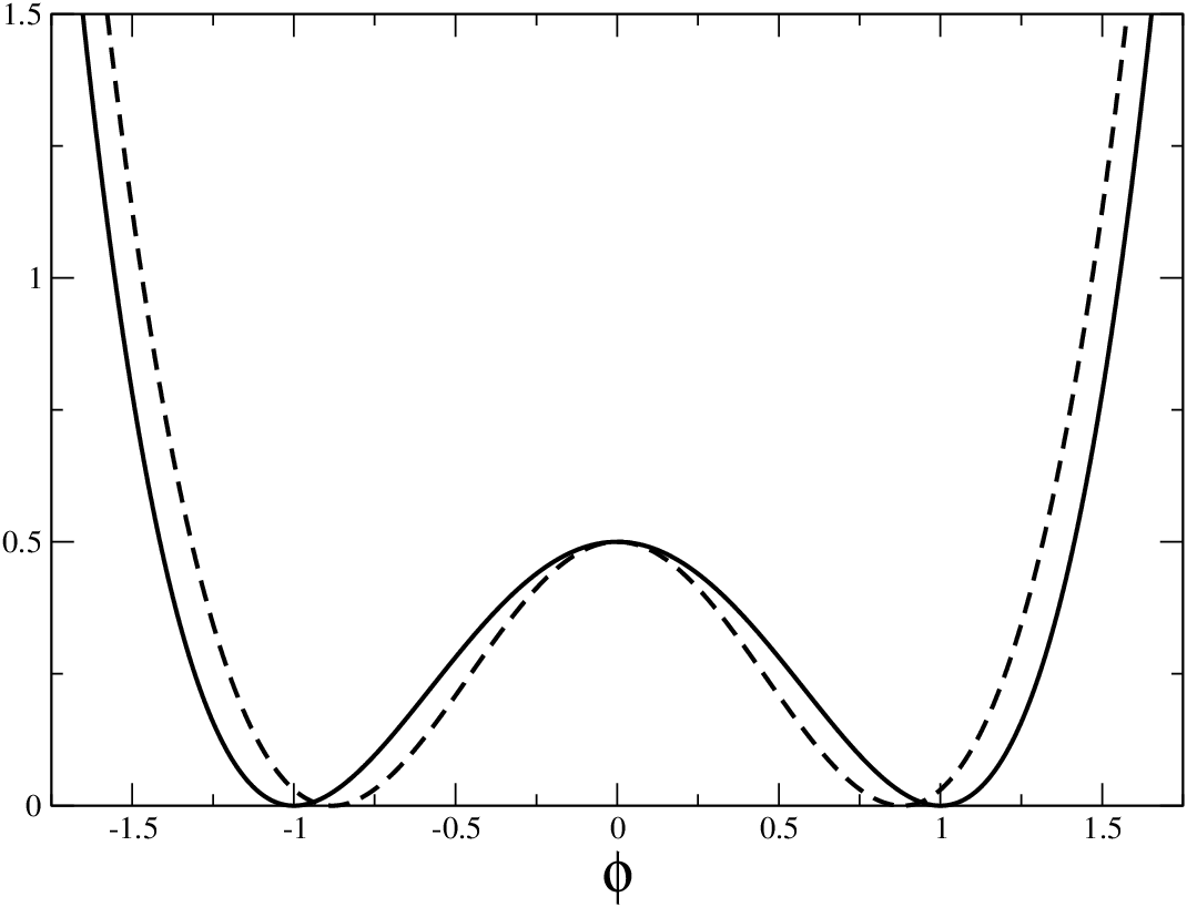
Shown in Figure 1(a) are the field potential of the polynomial and sinh-deformed functions of the model. That for the model for various values of are shown in Figure 2. There are two vacuum solutions in the sinh-deformed model, as observed in Figure 1(a), but for the sinh-deformed model, three cases emerges. For , we observe three degenerate minima at and , see Figure 2(a).
For , we observed in Figure 2(b) an additional local minimum at and finally, for we observe in Figure 2(c) two degenerate minima at . The models in Eq. (23) possesses a discrete symmetry () that is broken by the perturbative vacua (respectively, in all three cases of the sinh-deformed model).
Applying Eq.(9) to the kink-antikink solutions of the polynomial model Takyi:2016tnc the kink-antikink solutions of the sinh-deformed model are
| (24) |
which are related by the spatial reflection . Shown in Figure 1(b) are the kink solutions of the sinh-deformed and polynomial model. The corresponding classical kink mass is
| (25) |
The background potential for the fluctuations, which defines the excitation spectrum of the kink, is symmetric under the spatial reflection
| (26) |
This yield , with as observed in Figure 3.


In the sinh-deformed model, we obtain the kink solution for as Weigel:2017iup; Lohe:1979mh
| (27) |
where . The kink solution for is indicated in Figure 4(a). The spatial reflection gives the antikink. The background potential is
| (28) |
and is symmetric under the spatial reflection as observed in Figure 5(a) for . Consequently, .
For , two distinct kink solutions exist Takyi:2016tnc; Dorey:2011yw. The first one interpolates between and
| (29) |
which we show in Figure 4(b), while the second one interpolates between and (see Figure 4(c)),
| (30) |
The corresponding classical kink mass in either case is
| (31) |
The background potential for the fluctuations in this case is not symmetric under the spatial reflection
| (32) |
This, of course, implies that as observed in Figure 5(b). In the same figure we also show the corresponding pseudo-potential.
IV.2 The Hyperbolic Model
Here we consider the hyperbolic potential Bazeia:2018qur
| (33) |
This potential has two degenerate minima as observed in Figure 6(a). In the limit of small values of , this potential approaches the polynomial model
| (34) |
with a factor compared to in Eq. (22). The kink-antikink solutions of the hyperbolic model are
| (35) |
which are related by the spatial reflection . The kink solution is shown in Figure 6(b). The resulting classical mass is
| (36) |
The background potential
| (37) |
is symmetric under the spatial reflection as observed in Figure 7. In the limit as we have .


V Numerical Results
In this section, we report our numerical results for the VPEs for the two models discussed above. As stated earlier, we have rescaled to dimensionless coordinates and fields such that model parameters (coupling constant ‘’ and mass ‘’) are unity. It must be noted that the coupling constant serves as a loop-counting parameter. In this case, the classical mass scales as while the VPE proportional to , where is a mass parameter 11 1 This generally holds for the model. For this to be correct, for the model the dimensionless parameter must be written as where do not vary with or . Then the quadratic mass type term in does not contain the coupling constant . in the potentials considered. Thus, taking the coupling constant as unity does not affect the computation of the VPE.

We obtain the bound states energies contribution to the VPE, by first solving the Schrödinger-wave equation using the Boole’s algorithm, which is otherwise know as the -point closed Newton-Cote formula; with the initial conditions
and
from either side. We obtained the bound state energy by tuning the energy such that the Wronskian is zero at the matching point .
The next step requires computing the continuum part of the VPE, where the phase shift and its first Born approximation are obtained by solving Eqs. (11) and (18). We achieved this by utilizing the Runge Kunta algorithm to solve Eq. (14) which yields the S-matrix needed for the computation of the phase shift. It must be noted that the numerically obtained phase shift does not vary with the choice of .
We will be looking at two scenarios in the computation of the VPE. The first case deals with models with symmetric scattering potential. This regime, has equivalent vacua at , as such translating the kink solution as22 2 This corresponds to kink solution centered at . does not change the VPE of the kink. For models with asymmetric scattering potential, the non-equivalent vacua produce translational variance with the center of the kink solution .
V.1 The Sinh-Deformed Models
We first compare the results of the sinh-deformed model and its corresponding polynomial model. The two vacua for both models have equal curvature with . From Figure 3, one observes that the scattering potential of the polynomial model is shallower and broader than that of the polynomial model. We observed that both cases have two bound states with the bound state energies of the polynomial model smaller than that of the corresponding sinh-deformed model; this is attributed to the shallowness and broadness of its scattering potential. This in effect accounts for the smaller value of the VPE observed in the polynomial model as indicated in Table 1. Figure 8(a) shows the phase shift for the sinh-deformed model, confirming the Levinson’s theorem cf. Eq. 17 for .
bound state energies polynomial 0.0 1.732 -1.134 0.470 -0.664(-0.666) sinh-deformed 0.0 1.892 -1.054 0.412 -0.643(-0.644)
polynomial 0.154 0.053 -0.047 -0.148 -0.249 sinh-deformed 0.229 0.129 0.028 -0.074 -0176
polynomial Jost (poly. ) Error (poly. ) sinh-deformed Jost (sinh-def. ) Error (sinh-def. )
In the case of sinh-deformed model for , we have an asymmetric scattering potential with an unequal meson masses and for the kink soliton cf. Eq. (29). We observed from Figure 5(b) for that the scattering potential is narrower and almost overlap that of its polynomial counterpart. This in turn causes its VPE to be large cf. Table 2. Furthermore, the results indicate that except for the zero-mode there will be no additional bound state. We numerically obtained the binding energy (denoted by ), as which is larger than the binding energy, of the polynomial model. The unequal meson masses produces a translational variance of the VPE as seen in Table 2 under the translation . The results show that as increases, the kink shifts the vacuum with the bigger mass towards negative infinity causing low-lying modes to disappear. This decreases the VPE. It must be noted that the results stem from a change in values of the phase shift as varies. The phase shift exhibits the threshold scattering cusp and approaches as confirming Levinson’s theorem. We verified this by the plot of the phase shift in Figure 8(d).
For we observe a symmetric scattering potential cf. of Figure 5(a). This potential is narrower compared to that of the polynomial model. In effect, it yields large values for the VPEs for various values of as seen in Table 3. The results in Table 3 show that the results using the Jost function formalism of Eq. (20) agrees favorable well with the present calculations of Eq. (19) with a minor error. The error margin improves as increases. Here the error is estimated as the relative error . Also, we show in Figure 8(c) the phase shift for .
V.2 The Hyperbolic Model

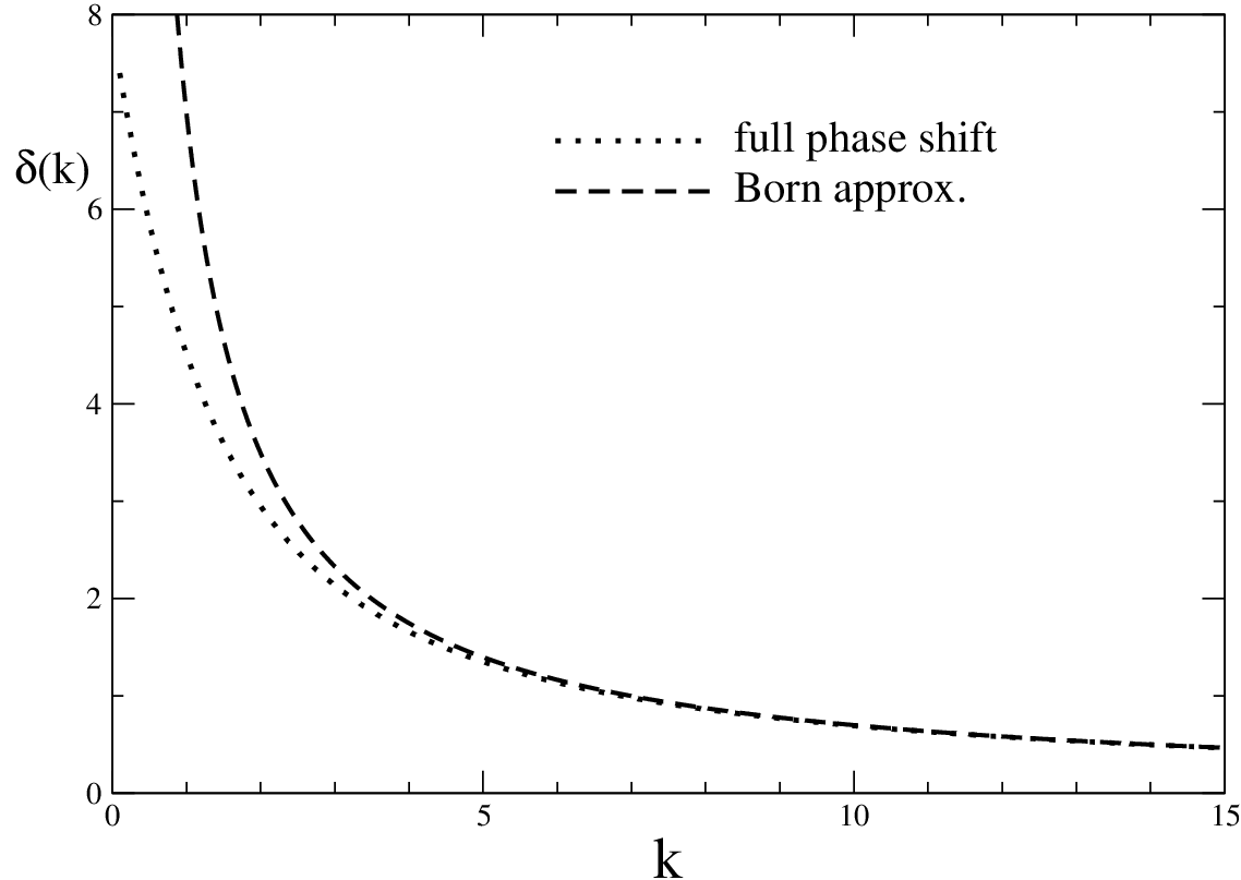


We observe that the scattering potential of the hyperbolic model is symmetric and broader than its corresponding polynomial model cf. Figure 7. This causes its VPE to be smaller compared to the polynomial counterpart as seen in Table 4. Also, we observe two vibrational modes in addition to the translational zero-mode compared to the one vibrational mode of its polynomial model. The occurrence of this is due to the broadness of its scattering potential. Also, the VPE result from calculations of the hyperbolic model is in agreement (within numerical precision) to the one obtained by using the heat kernel method AlonsoIzquierdo:2011dy; AlonsoIzquierdo:2012tw. The result from the heat kernel method has the value of VPE as . Finally, in Figure 8(b), we show the phase shift for this model for , thus confirming the Levinson’s theorem.
VI Conclusion
We have investigated the vacuum polarization energies (VPE) of kinks in the sinh-deformed and models obtained from the polynomial and models by a deformation procedure. We make use of spectral methods for computing the VPE in terms of scattering data for the quantum fluctuations about the classical kink. The models we used are not multiplicatively renormalizable. However, using the no-tadpole renormalization condition at one-loop order produce finite results for our calculations.
bound state energies polynomial 0.0 1.225 -0.802 0.354 -0.448(-0.471) hyperbolic 0.0 1.433 1.911 -1.328 0.597 -0.732(-0.734)
Our results show that the sinh-deformed and models show similar behaviors to their polynomial counterparts. In the case of the model they both have two bound states; the zero-mode and a vibrational shape mode. The narrowness of the scattering potential of the sinh-deformed model causes its vibrational mode frequency to be larger than that of its polynomial counterpart. In effect, the VPE of the sinh-deformed model is quite large. In the case of the model with the dimensionless parameter , the kink solutions of both models possesses non-equivalent vacua at spatial infinity. This leads to translational variance with respect to the center of the kink. The VPE may assume any negative value which then destabilizes the kink. The broadness of the scattering potential of the polynomial model in this case, causes its binding energy to be smaller than that of the sinh-deformed model.
In the case of the hyperbolic model, we find its scattering potential to be broader than its polynomial counterpart. We also observe two vibrational modes for the hyperbolic model as compared to only one for its polynomial counterpart. In effect, the VPE of the hyperbolic model is smaller. The reported value of the VPE in this case, is which is in agreement with the value reported using the heat kernel method. The later approach makes use of function regularization which requires truncation approximation.
It will be interesting to study the VPEs as a function of the kink-antikink potentials of the sinh-deformed models as well as the hyperbolic model. To do this requires to first substitute the configuration of the kink-antikink solutions that describe its scattering interactions to the Lagrangian density to obtain the classical kink potential. The VPE is then computed using the obtained potential. In deriving this configuration care must be taken in such a way that the configuration is not a solution to the stationary equations and additions must be made to avoid an imaginary VPE.
Acknowledgment
We are grateful to H. Weigel for stimulating discussions and helpful comments on the manuscripts.
References
- (1) R. Rajaraman. Solitons and Instantons. North Holland, 1982.
- (2) T. H. R. Skyrme. The origins of Skyrmions. Int. J. Mod. Phys. A 3, 2745 (1988) 2745. Article reconstructed by I. Aitchison.
- (3) G. S. Adkins, C. R. Nappi, and E. Witten. Static properties of nucleons in the Skyrme model. Nuclear Physics B 1983; 228(3): 552-566. doi: 10.1016/0550-3213(83)90559-X
- (4) H. Weigel. Chiral soliton models for baryons. (Vol. 743), Springer-Verlag, 2008.
- (5) E. F. Meoto, M. L. Lekala, G. J. Rampho and B. Mukeru. Atomic binding energies for the ground state of some helium-like hypernuclear atoms. Journal Physics G 2019; 46(9): 095102. doi: 10.1088/1361-6471/ab26f2
- (6) N. Graham, M. Quandt and H. Weigel. Spectral methods in quantum field theory. (Vol. 777), Springer-Verlag, 2009.
- (7) R. F. Dashen, B. Hasslacher and A. Neveu. Nonperturbative methods and extended-hadron models in field theory II. Two-dimensional models and extended hadrons. Physical Review D 1974; 10(12): 4130–4138. doi: 10.1103/PhysRevD.10.4130
- (8) R. F. Dashen, B. Hasslacher and A. Neveu. Particle spectrum in model field theories from semiclassical functional integral techniques. Physical Review D 1975; 11(12): 3424-3450. doi: 10.1103/PhysRevD.11.3424
- (9) L. D. Faddeev and V. E. Korepin. Quantum theory of solitons. Physics Report 1978; 42(1): 1-87. doi: 10.1016/0370-1573(78)90058-3
- (10) B. Moussallam and D. Kalafatis. On the Casimir energy of a skyrmion. Physics Letters B 1991; 272(3): 196-201. doi: 10.1016/0370-2693(91)91819-H
- (11) G. Holzwarth and H. Walliser. Quantum corrections to the skyrmion mass Nuclear Physics A 1995; 587(4): 721-746. doi: 10.1016/0375-9474(95)00012-P
- (12) F. Meier and H. Walliser. Quantum corrections to baryon properties in chiral soliton models. Physics Report 1997; 289(6): 383-448. doi: 10.1016/S0370-1573(97)00012-4
- (13) A. Achúcarro and T. Vachaspati. Semilocal and electroweak strings. Physics Report 2000; 327(6): 347-426. doi: 10.1016/S0370-1573(99)00103-9
- (14) H. Weigel. Emerging Translational Variance: Vacuum Polarization Energy of the Kink. Advances in High Energy Physics 2017; 2017: 1486912. doi: 10.1155/2017/1486912
- (15) H. Weigel. Vacuum Polarization Energy for General Backgrounds in One Space Dimension. Physics Letters B 2017; 766: 65-70. doi: 10.1016/j.physletb.2016.12.055
- (16) I. Takyi, M. K. Matfunjwa and H. Weigel. Quantum Corrections to Solitons in the Model. Physics Review D 2020; 102(11): 116004. doi: 10.1103/PhysRevD.102.116004
- (17) D. Bazeia, E. Belendryasova and V. A. Gani. Scattering of kinks of the sinh-deformed model. European Physics Journal C 2018; 78(4): 340. doi: 10.1140/epjc/s10052-018-5815-z
- (18) D. Bazeia, A. R. Gomes, K. Z. Nobrega, F. C. Simas. Kink scattering in hyperbolic models. International Journal Modern Physics A 2019; 34(31): 1950200. doi: 10.1142/S0217751X19502002
- (19) I. Takyi and H. Weigel. Collective Coordinates in One-Dimensional Soliton Models Revisited. Physics Review D 2016; 94(8): 085008. doi: 10.1103/PhysRevD.94.085008
- (20) H. Weigel. Kink-Antikink Scattering in and Models. Journal of Physics Conference Series 2014; 482: 012045. doi: 10.1088/1742-6596/482/1/012045
- (21) P. Anninos, S. Oliveira, R. H. Matzner. Fractal structure in the scalar theory. Physics Review D 1991; 44: 1147–1160. doi: 10.1103/PhysRevD.44.1147
- (22) D. K. Cambell, J. F. Schonfeld and C. A. Wingate. Resonance structure in kink-antikink interactions in theory. Physica D 1983; 9(2): 1-32.
- (23) P. Dorey, K. Mersh, T. Romanczukiewicz, Y. Shnir. Kink-antikink collisions in the model. Physics Review Letters 2011; 107(9): 091602. doi: 10.1103/PhysRevLett.107.091602
- (24) D. Bazeia, M. A. González León, L. Losano and J. M. Guilarte. Deformed defects for scalar fields with polynomial interactions. Physics Review D 2006; 73(10): 105008. doi: 10.1103/PhysRevD.73.105008
- (25) D. Bazeia, L. Losano and J. M. C. Malbouisson. Deformed defects. Physics Review D 2002; 66(10): 101701. doi: 10.1103/PhysRevD.66.101701
- (26) C. A. Almeida, D. Bazeia, L. Losano and J. M. C. Malbouisson. New results for deformed defects. Physics Review D 2004; 69(6): 067702. doi: 10.1103/PhysRevD.69.067702
- (27) D. Bazeia and L. Losano. Deformed defects with applications to braneworlds. Physics Review D 2006; 73: 025016. doi: 10.1103/PhysRevD.73.025016
- (28) D. Bazeia, E. E. M. Lima and L. Losano. Kinks and branes in models with hyperbolic interactions. International Journal of Modern Physics A 2017; 32(26): 1750163. doi: 10.1142/S0217751X17501639
- (29) F. Calegero. Variable Phase Approach to Potential Scattering. Academic Press, New York and London, 1967.
- (30) M. A. Lohe. Soliton structures in ) in two-dimensions. Physics Review D 1979; 20(12): 3120. doi: 10.1103/PhysRevD.20.3120
- (31) D. Bazeia, D. A. Ferreira, E. E. M. Lima and L. Losano. Novel results for kinklike structures and their connections to quantum mechanics. Annals of Physics 2018; 395: 275–300. doi: 10.1016/j.aop.2018.06.006
- (32) A. Alonso-Izquierdo and J. Mateos Guilarte. One-loop kink mass shifts: A Computational approach. Nuclear Physics B 2011; 852: 696-735. doi: 10.1016/j.nuclphysb.2011.07.005
- (33) A. Alonso-Izquierdo and J. Mateos Guilarte. On a family of (1+1)-dimensional scalar field theory models: kinks, stability, one-loop mass shifts. Annals of Physics 2012; 327: 2251-2274. doi: 10.1016/j.aop.2012.04.014
- (34) T. Vachaspati. Kinks and domain walls: An introduction to classical and quantum solitons. Cambridge University Press, 2010.
- (35) A. Vilenkin and E. P. S. Shellard. Cosmic Strings and Other Topological Defects. Cambridge University Press, 2000.
- (36) T. Romańczukiewicz. Could the primordial radiation be responsible for vanishing of topological defects? Physics Letters B 2017; 773: 295-299. doi: 10.1016/j.physletb.2017.08.045
- (37) A. R. Bishop, J. A. Krumhansl and S. E. Trullinger. s in condensed matter: a paradigm. Berlin: Springer Verlag, 1980.
- (38) P. G. Kevrekidis, D. J. Frantzeskakis and R. Carretero-González. Emergent Nonlinear Phenomena in Bose-Einstein Condensates: Theory and Experiment. Berlin: Springer Verlag, 2008.
- (39) B. Ivanov, A. Kichiziev, Y. N. Mitsai. Nonlinear dynamics and relaxation of strongly anisotropic ferromagnets. Soviet Physics JETP 1992; 75: 329-337.
- (40) S.-H. Dong, X.-W. Hou, Z.-Q. Ma. The Relativistic Levinson theorem in two-dimensions. Physical Review A 1998; 58: 2160. doi: 10.1103/PhysRevA.58.2160