In previous papers [4][5] the Majorana-SYK model was compared with the dynamics of neutral particles in a background of a dimensionally reduced Reissner-Nordstrom black hole. In this paper we will replace the Reissner-Nordstrom background with the closely related but slightly simpler solution of the $(1+1)$-dimensional dilaton-gravity theory discussed in [10]. The model is a variant of the Jackiw-Teitelboim (JT) theory described by the action,

where $\Phi_{0}$ is a dimensionless constant, $\phi$ is a dynamical field, BT stands for a boundary term, and MT stands for matter terms. The term proportional to $\Phi_{0}$ is topological and determines the zero-temperature extremal entropy. We will define the dilaton field $\Phi$ by,

The parameter $\mu$ has units of length and determines the radius of curvature of the $AdS(2)$ solution.

The variational equation for $\phi$ requires the curvature to be constant,

and the equations generated by variation with respect to the metric are,

which, together with boundary conditions, determine $\phi.$

The solution of the equations of motion for the metric is $AdS(2)$ which can be written in the form,

The point $r=\mu$ represents the horizon but unlike in higher dimensions the coordinate $r$ does not signify the radius of a sphere. Nor is its value at the horizon related to entropy. In JT-gravity that role is played by the dilaton field $\Phi(r)$ whose value at the horizon determines the entropy according to,

The JT equations of motion of the dilaton field are solved by the sum of the constant term $\Phi_{0}$ and a varying part $\phi(r)$ which varies according to,

The factor of proportionality $c(\beta)$ in is temperature dependent and will be fixed in section 4.

The proper distance from the horizon will be called $\sigma,$

from which we find,

The metric takes the form,

Defining $y=\sigma/\mu$ and $t/\mu=i\theta$ the Euclidean continuation has the familiar form of the hyperbolic disc,

In the model of [10] the geometry ends at a boundary located at the value of the radial variable $y$ at which the circumference of the circle $(0<\theta\leq 2\pi)$ is the inverse temperature $\beta,$

The subscript $b$ stands for boundary. (See figure 1)

In terms of $\sigma$ the boundary is at

For large $\beta$ (low temperature),

The time coordinate $t$ is not the proper time of an observer at the boundary. Following [10] we denote the boundary proper time by $u.$ The relation between $t$ and $u$ is,

When considering the relation between JT gravity and the holographic SYK system, the usual convention is that the time conjugate to the SYK Hamiltonian is $u.$

It is convenient when studying the motion of a particle that falls in from the boundary to introduce a coordinate which measures proper distance from the boundary. Calling it $\rho,$

The $AdS(2)$ spatial geometry and the coordinates $\sigma\ \rho$ are shown in figure 2.

A particle dropped from the boundary will very quickly become relativistic and move on an almost light-like trajectory. A light-like trajectory originating at the boundary ($\rho=0$) at time $u=0$ will satisfy,

It is easy to show that it will reach the Rindler region in a time $\beta/2\pi.$ Assuming $\beta>>\mu$ then for almost all of that time the trajectory will be in the throat region.

Equation 2.16 can be used to convert a function of spatial position $f(\rho)$ to a function of time $f(u)$ along an infalling trajectory. In particular the function $\tilde{\beta}(\rho)$ introduced in [4][5] may be thought of as a function of time along the trajectory of an infalling relativistic particle.

We will begin by deriving the equation of motion of a particle moving in the metric,

and an abelian gauge field of the form,

Here $E$ is constant and represents a uniform electric field and $r_{b}$ is the value of $r$ at the boundary.

The standard Lagrangian is,

where dot means derivative with respect to $t.$

The momentum conjugate to $\rho$ is given by,

and the Hamiltonian by,

Note that the Hamiltonian $H_{t}$ is conjugate to $t$ and not to the boundary time $u.$ The Hamiltonian conjugate to boundary time will simply be denoted by $H$ without any subscript. The relation between $H$ and $H_{t}$ is,

The radial force $F_{t}$ on the particle is defined to be $dP/dt$ and is given by,

From 3.11 we find,

The force $F_{t}$ represents the rate of change of momentum $P$ with respect to $t,$

The rate of change of $P$ with respect to boundary time will be denoted without a subscript,

Thus one finds,

where

The subscripts $G$ and $E$ refer to gravitational and electric.

Using 2.13, 2.14, 2.15, and 3.6, in the throat region equation 3.27 may be written as,

The factors of $e^{-\rho/\mu}$ in 3.32 go to zero as we move away from the boundary at $\rho=0.$ In particular this means that $F_{G}$ quickly tends to a constant value

while $F_{E}$ rapidly decreases as the particle moves away from the boundary.

For an electrically neutral particle the force has the simpler form,

In the Majorana-SYK theory acting with a fermion operator $\psi$ at time $u=0$ creates a particle at rest at the boundary, which subsequently falls into the throat. The Heisenberg operator $\psi(u)$ initially has size $1$. The size grows with time, but the energy is conserved. This is the process described below by the Qi-Streicher formula 4.2. The energy of such an initial size-$1$ particle is what we have been calling $H$ in equations like 3.33.

As we will discuss in section 5 the momentum-size correspondence can be expressed in the form [6][5],

where ${\cal{C}}(t)$ is the size of the operator $\psi(t).$

Qi and Streicher [9] have calculated the size of $\psi(u)$ in Majorana-SYK to be,

From 4.1 and 4.2 we find that in the throat,

and the force which is defined as $dP/du$ is given by the constant value,

From 3.33 and 4.4 we obtain the following expression for $H$,

To determine $\mu$ in terms of SYK parameters we turn to black hole thermodynamics and compare the specific heat of a near-extremal black hole with that of the SYK model.

We would like to express $\mu$ in terms of the SYK parameters $N,{\cal{J}},q.$ To do so we will equate the zero-temperature specific heat of the JT gravity solution with the corresponding SYK result. We begin with the dilaton which plays the role of area in JT. The dilaton has a constant background part $\Phi_{0}$ and a varying part $\phi.$

The dilaton profile $\phi(\sigma)$ is determined by solving the equation of motion and setting the boundary value to a fixed constant of order $\Phi_{0}.$ The precise value is not important but for convenience we will choose,

One finds

The extremal entropy is given by

For large $q$ it has the value $\frac{1}{2}N\log{2}$. Thus,

The near-extremal entropy is given by $1/4G$ times the dilaton at the horizon which from 4.7 is,

where $T=1/\beta.$

Using 4.8,

To determine $\mu$ we use the SYK value for $dS/dT.$ In the large $q$ limit the SYK value has been calculated analytically [11],

Equating 4.10 and 4.11,

for large $q$.

Finally, having obtained $\mu$ in terms of SYK parameters, we may go back to 4.5 and obtain $H$,

We have treated the boundary as if it were frozen at $\sigma=\sigma_{b}$ with $\sigma_{b}$ given by 2.12. To put it another way, we have treated the boundary as if it has infinite mass. In practice that is a good approximation, but in fact the boundary is a dynamical object which can recoil and move when a force is applied to it. For example, when a particle is dropped in from the boundary the boundary will recoil so that its momentum will be equal and opposite to the momentum of the particle [5]. However, the boundary itself behaves as a very heavy non-relativistic particle whose mass is,

Using 4.12 we may write,

The fact that the boundary mass is order $N$ means that the recoil motion is usually negligible.

For $q>>1$ the relation between the JT and SYK variables that we will need is given by,

where in 4.24(c,d) the quantites $H$ and $F$ refer to the energy and the force on a size-1 particle in the throat.

At large $q$ the evolution of a single fermion operator is described by diagrams of the form shown in figure 3. The diagram represents the “branching diffusion” pattern shared by SYK and string theory. It is simplified so that it shows an uniform rate of branching with respect to some yet-to-be-determined time variable $\tau.$ This is an simplification which is only correct in an average sense but it’s good enough for our purposes. The time variable $\tau,$ which we will call “circuit time” is not assumed to be the boundary time $u$ or even linear³³ 3 The nonlinear relation between circuit and ordinary time was also necessary in the quantum-epidemic model of Qi and Streicher in order to reproduce the results of their calculation of growth. in $u.$

Identifying the number of endpoints (leaves of the tree) as the size ${\cal{C}}$ of the growing operator, the branching diffusion implies an exponential growth of size in $\tau$. In the $q$-local version of SYK a fermion will split into $(q-1)$ offspring. It is natural to write,

However by redefining $\tau$ we may eliminate the factor $(q-2)$ and write,

We have assumed ${\cal{C}}(0)=1$ in line with the fact that the initial fermion operator in the upcoming SYK calculation has size $1.$

As remarked above, the circuit time $\tau$ is not the usual asymptotic time $u,$ nor is it linear in $u$. One might think that 5.3 has no content other than as a definition of $\tau$ but that’s not true. The invariant fact expressed by figure 3 and equation 5.3 is that the number of leaves of the tree (the size) is proportional to the number of vertices. By analogy with quantum circuits the number of vertices represents the growing complexity of $\psi(t).$ This is the basis for the claim that size and complexity are proportional to one another.

Let us digress for a moment to explain why the circuit time is not proportional to the time $u$ conjugate to the SYK Hamiltonian. Consider the energy carried by each line in the diagram of figure 3. An incoming energy $\omega$ will split at each vertex so that the average energy carried by a line will decrease exponentially with $\tau.$ This naturally implies that the time $\Delta u$ to the next vertex will grow exponentially with $\tau.$ In terms of the epidemic model it means that the rate of contact between participants slows down in real time. This slowdown was noted in [5] where the time between vertices $\Delta\tau$ was denoted $\tilde{\beta}.$ It was also commented on in [9].

The proportionality of size and complexity can not go on forever. It and and the tree-like nature of the evolution must break down at the scrambling time when the size becomes comparable to the number of fermionic degrees of freedom, $N$. At that point the size saturates but the complexity continues to grow linearly with $u.$ But by this time the particle has long passed through the throat and is in the Rindler region.

We will assume that boundary time $u$ and circuit time $\tau$ are monotonically related,

Following [5] we define,

The first of equations 5.3 takes the form

In [5] a specific form of the momentum-size correspondence was proposed,

Combining 5.6 with 5.5 implies,

Equations 5.6 and 5.7 are two forms of the momentum-size correspondence which in the scaling region, i.e., the throat, are equivalent. Which of them is more fundamental is not obvious but the version 5.7 was derived in a rigorous manner from the $SL(2R)$ symmetry of AdS(2). Moreover it holds not only through the throat but also through the scrambling process in the Rindler region.

Note that one may start with 5.7 and reverse the argument to derive 5.6.

Let us consider the functional relation $u(\tau).$ One way to obtain it is to use the approximate scale invariance of SYK at low temperature. It implies that ${\cal{C}}(u)$ should be a power of $u$. Furthermore it should be time-symmetric and smooth at $u=0$. The simplest dimensionally consistent assumption is

with $c$ being a constant. Qi and Streicher [9] calculate that at large $q$ the size grows according to 4.2,

From 5.11 we read off that the constant in 5.8 is $c=2.$

Next we note that

so that

and from $du/{d\tau}=\tilde{\beta}$ we find,

where the factor ${{\cal{J}}}^{-1}$ is necessary for dimensional consistency and to match 5.11.

The conjectured momentum-size correspondence, if correct, would imply that the momentum is given by,

This may be interpreted in terms of a constant force $F$ acting on the particle,

which agrees with 4.4.

At this point we will digress very briefly to comment on the relation between the rate equation 5.3 and the ladder-sum for four-point out-of-time-order-correlators. The diagrams of figure 3 represent amplitudes which need to be squared in order to give probabilities. Accounting for the usual SYK disorder averaging the leading melon diagrams are like the one in the left panel of figure 4. In order to calculate the average size at a given time one needs to count the number of fermionic lines in the intermediate state. This is done by inserting the number operator⁴⁴ 4 The definition of the number operator that we use was given by Qi and Streicher [9]. The number operator is defined on two copies of the $N$ fermion system which are identified with the bra and ket sides of the diagrams in figure 3. $[(\psi_{i})_{L},(\psi_{i})_{R}]$ according to the prescription in [9]. Diagrammatically it is denoted by the open gap on one of the intermediate lines. The open gap can be on any of the intermediate lines and the sum over such diagrams represents the probability for a given size.

In fact the symmetry of the diagram is such that the sum just gives a multiplicative factor equal to the number of fermion lines.

The relation with four-point ladder diagrams is clear if we redraw the left panel in the equivalent form in the right panel. The two diagrams are equivalent but the right panel has been drawn to emphasize the ladder-like nature of the graphs.

One question that figure 4 raises is why the lower rungs of the ladder have more internal structure than the upper rungs. The answer is that in the model with uniform spacing of vertices in $\tau$ the circuit time between the beginning and end of a rung is greatest at the bottom of the ladder and grows smaller as we proceed up the ladder. The actual ladder kernal is a sum of diagrams, but which diagram dominates depends on the time-interval between where it connects with the rails.

From the ladder diagram point of view the exponential growth of the size is characteristic of the graviton Regge trajectory.

The vertices governing the growth of size are shown in figure 5.

To vary the charge of the black hole a chemical potential $\nu$ is introduced⁶⁶ 6 In our convention the chemical potential is dimensionless in contrast to the usual convention in which it has units of energy. into the thermal density matrix as an extra factor $e^{\nu(n_{+}-n_{-})},$ where $(n_{+}-n_{-})$ is the total fermion charge. It’s effect is to modify the bare propagators connecting the vertices. A line labeled $\pm$ carries a factor $e^{\mp\nu}$ as in figure 5

Let us see how these factors comes about. The bare propagators are defined in the non-interacting theory (${\cal{J}}=0$) in which the different fermionic coordinates do not interact. Therefore it is sufficient to concentrate on a single complex fermionic degree of freedom. We may think of the fermionic system in terms of Pauli matrices,

The bare propagator is defined in terms of the non-interacting two-point function,

where the density matrix is

One finds,

Thus a line representing a positive fermion carries a factor $\frac{e^{\nu/2}}{2}$ and a line representing a negative fermion carries a factor $\frac{e^{-\nu/2}}{2}$.

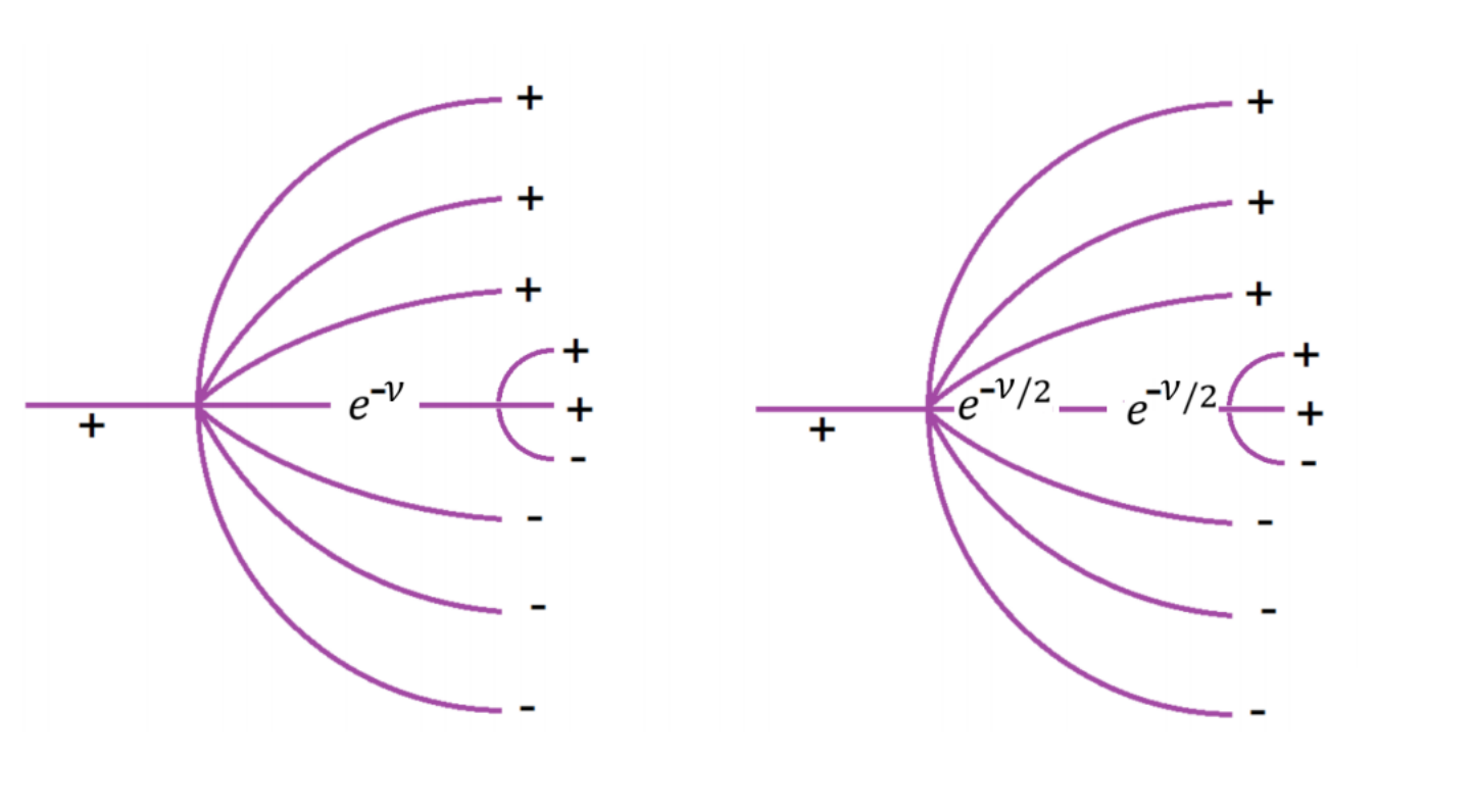
It is convenient to redistribute these factors by splitting each $e^{\pm\nu/2}$ into two factors $e^{\pm\nu/4}e^{\pm\nu/4}$ and bringing them to the vertices as in figure 6. when this is done each vertex with an incoming $\pm$ line will be weighted with a factor $e^{\pm\nu/2}.$ In addition the entire graph will have an overall factor $e^{\nu/2}$ which does not depend on the graph. The coupling ${\cal{J}}$ governing the strength of each vertex is thereby “renormalized ” from ${\cal{J}}$ to $e^{\pm\nu/2}{\cal{J}}.$ This is indicated in figure 5.

The factors $e^{\pm\nu/2}$ occur in amplitudes—roughly speaking, the amplitude that the initial fermionic perturbation evolves to a given number of positive and negative constituents—but the rate equations in the next section are about probabilities. This means that in the weighting of each graph the factors $e^{\pm\nu/2}$ must be squared to give a weight $e^{\pm\nu}$ to each vertex.

Equation 5.3 is the simplest possible rate equation that one can write down. In the case of $U(1)$-SYK the equations are similar but more complicated since one has to keep track of two species of fermions—those with positive charge and those with negative charge.

Define the partial sizes $n_{\pm}$ to be the average number of $\pm$ charged fermions in an operator. The total size $(n_{+}+n_{-})$ will again be denoted ${\cal{C}}.$ If the process is initiated by a $\pm$ charged fermion operator, then the size after circuit time $\tau$ will be denoted by ${\cal{C}}(\tau)_{\pm}$. Specifically the size of $\psi^{{\dagger}}(\tau)$ is ${\cal{C}}(\tau)_{+}$ and similarly the size of $\psi(\tau)$ is ${\cal{C}}(\tau)_{-}$.

The rate equations for the tree-like graphs that dominate the large $q$ model should have several properties:

1. 1.

   They should be linear. Once a splitting has occurred the different branches do not interact.

2. 2.

   For reasons explained above, the splitting of a $\pm$ fermion should be weighted by a probability $e^{\mp\nu.}$ This is indicated in figure 5.

3. 3.

   The equations should conserve the value of $(n_{+}-n_{-}).$ This is to insure charge conservation.

The most general rate equation with these properties is,

The eigenvalues and eigenvectors⁷⁷ 7 The ket-like notation here does not indicate a quantum state, but only the real column vector whose entries are $n_{+},n_{-}.$ of the matrix in 6.16 are,

We will be interested in solutions of the rate equations in which the initial state is either one positive or one negative fermion. We denote these initial states by $|\psi(0))_{\pm}.$ By definition,

The solution of the rate equations with these initial conditions is,

and finally,

In general when we compare with the GR calculation the presence of a chemical potential will back-react and influence the metric, but by working to lowest order in in $\nu$ back-reaction can be ignored. Thus from now on we will work to linear order in $\nu,$

This is the total size for an initial state with one ${\pm}$ fermion.

Using 5.13 we find the sizes as a function of $u$,

For ${\cal{J}}u>1$ the second term may be ignored compared to the first,

As an example consider the size of a positively charged operator ${\cal{C}}_{+}$ assuming the chemical potential is positive. From 6.31 we see that the growth is slowed relative to the case with $\nu=0.$ Since with our convention a positive chemical potential will induce a positive charge, the result implies that like-sign charges retard the operator growth. Similarly opposite charge increases the growth rate. This of course is the holographic equivalent of like-signs repel, unlike signs attract.

The time dependence of size is rigorously quantified by the evolution of the 4-point out-of-order-correlator. In SYK these OTOCS are dominated by ladder diagrams which are evaluated by iterating a ladder kernel. The ladders are described by Regge behavior with Regge intercepts given in terms of the eigenvalues of the kernel.

The matrix in the rate equations 6.16 is a simplified version of this kernel. In the limit $\nu\to 0$ the two eigenvalues in 6.23 are $\lambda_{1}=0$ and $\lambda_{2}=1.$ The second is already present in Majorana-SYK and corresponds to the graviton trajectory. The first is a new feature of $U(1)$-SYK and corresponds to the photon trajectory.

In the large $q^{2},$ fixed $\beta{\cal{J}}$ limit the charge of the system and the chemical potential are related by,

Equation 6.32 together with

imply that equation 6.31 can be re-written in terms of the black hole mass and the integer-valued $U(1)$ generator $Q.$

Concerning equation 6.32, it is true in the weak coupling limit and therefore in the limit $q^{2}>>\beta{\cal{J}}.$ It may be derived in the free fermion limit. To see that consider the partition function for a single free fermion mode,

The charge $Q$ to first order in $\nu$ is given by,

Extending this to $N$ fermionic modes gives 6.32.

Equation 6.32 is correct only correct for $q^{2}>>\beta J$ and must be significantly modified in the more interesting limit of fixed $q$ and very large $\beta{\cal{J}}.$ We will discuss this in section 8.

By using the momentum-size correspondence we will compare 6.34 with a general relativity calculation of the motion of charges in a NERN background. For the purpose of that comparison we note that the momentum-size correspondence applied to 6.34 would give,

In equation 6.32 $Q$ is not exactly the electric charge. $Q$ is the difference $(n_{+}-n_{-})$ which we do expect to be proportional to the electric charge, but with a factor of proportionality yet to be determined. Let us call the electric charge $\tilde{Q}.$ It differs from the integer-valued $U(1)$ generator by a factor $|e|$ representing the fundamental unit of charge,

There is something puzzling about equations 3.19 and 3.20 (it puzzled me); namely the presence of the term

in the expression for the gravitational force. Being proportional to the charge it would seem to be part of the electric force, but that would be very odd since the usual expression for electric force involves only the spatial derivative of $A_{u}.$ In fact the term,

was identified as the electric force in 3.27. It is also the term we dropped from 3.32 because it quickly becomes negligible as the particle moves away from the boundary. However, it would be a mistake to ignore it altogether.

The resolution of the puzzle is the following: The particle initially experiences an electric force $-e\partial_{\rho}A_{u}$ as an impulse as it starts out at $\rho=0.$ The impulse, although short-lived, affects the momentum and kinetic energy of the particle. By the time the particle has moved a distance $\sim\mu,$ depending on the relative sign of the particle and black hole, the electric impulse will have resulted in the particle having greater or lesser energy than a corresponding neutral particle. After the initial kick kinetic energy will be $H+eA_{u}.$

On the other hand the gravitational force on the particle is proportional to its kinetic energy, so depending on the sign of the charge, once the particle gets away from the boundary the gravitational force will either be less than or greater than that of the corresponding neutral particle. We see that the origin of the term proportional to $(H+eA_{u})$ is gravitational.

That the electric force $-e\partial_{\rho}A_{u},$ decreases quickly compared to the gravitational force is expected from Regge theory⁸⁸ 8 From the Regge-pole point of view, gravity corresponds to a trajectory with intercept $2$ while electromagnetism corresponds to a trajectory with intercept $1.$ In the current context this implies a dominance of gravitational force over electric force as the particle gains energy in the throat. .

Now we come to the main point: the comparison of the forces and acceleration of charged particles in the throat, and the growth of operator size in $U(1)$-SYK. From the general relativity calculation 7.7 we conclude that the momentum $P$ of an infalling charge is given by 7.8,

On the other hand let us return to the rate equations in section 6. The result was equation 6.34 for the growth of size, and (assuming the momentum-size correspondence) 6.43 for the growth of momentum. It is evident that 7.8 and 6.43 have similar form. Equating them we find,

Equation 7.9 is new information that fixes the fundamental unit electric charge, in other words the charge of a fundamental $U(1)$-SYK fermion. The fact that it is order $1/N$ means that electric forces are $1/N$ effects which may seem surprising. In the next section we will see that this has a simple explanation.

While 7.9 may seem surprising it is in fact entirely natural. What it suggests is that the $U(1)$-SYK system is a realization of Kaluza-Klein theory with a compactification scale which we might have guessed.

Let us add an additional compact KK direction so that the geometry becomes $AdS(2)\times U(1),$ with the compact circle having radius $R_{k}.$ The unit of electric charge in such a theory would be given by,

From 4.8 we see that

Comparing this with 7.9 we find,

The scaling of $R_{k}$ with $1/{\cal{J}}$ is hardly surprising since ${\cal{J}}^{-1}$ is the only length scale that appears in SYK. In principle $R_{k}$ might have had some uncancelled $N$ dependence, but that did not happen. The lack of $q$ dependence in $R_{k}$ is also interesting. We may compare 7.12 with 4.12,

We see that $R_{k}$ grows relative to the $AdS(2)$ length scale as $q$ increases. The significance of this is not entirely clear and one might wonder if it is an artifact of weak coupling, not to be trusted for fixed $q$ and large $\beta{\cal{J}}.$ In the next section⁹⁹ 9 The argument of section 7.4 is due to Henry Lin and Geoff Penington. evidence will be given that 7.13 is robust in the strong coupling limit $1<<q^{2}<<\beta{\cal{J}}.$

The arguments of the previous sections were derived from the weak coupling limit in which $\beta{\cal{J}}$ is held fixed and $q^{2}\to\infty.$ Nevertheless I believe the results—in particular the scaling of the KK radius 7.12—may be extrapolated to the strong coupling limit in which $q^{2}$ is held fixed and $\beta{\cal{J}}\to\infty.$

A method which is valid at strong coupling is the boundary particle description [10]. In this section we will use the boundary particle description to compute $R_{k}$ and see that it is indeed given by 7.12.

In the Majorana case the boundary particle has a single degree of freedom, i.e., its proper distance from the horizon. It moves nonrelativistically with a large mass, $M=N{\cal{J}}q^{2}$ (see 4.24-d). In $U(1)$-SYK the particle has a second $U(1)$ angular degree of freedom. The radial direction is frozen by a potential but the angular direction is a zero-mode. The quantized momentum conjugate to the angular coordinate is the integer-valued charge $Q.$

Because of the large mass of the boundary particle the Hamiltonian for the angular motion is non-relativistic,

We consider the thermal ensemble,

Completing the square and integrating over $n$ gives a partition function,

The charge $Q$ is given by,

References

- [1] D. A. Roberts, D. Stanford and A. Streicher, “Operator growth in the SYK model,” JHEP 06, 122 (2018) doi:10.1007/JHEP06(2018)122 [arXiv:1802.02633 [hep-th]].
- [2] S. Xu, L. Susskind, Y. Su and B. Swingle, “A Sparse Model of Quantum Holography,” [arXiv:2008.02303 [cond-mat.str-el]].
- [3] L. Susskind, “Why do Things Fall?,” [arXiv:1802.01198 [hep-th]].
- [4] A. R. Brown, H. Gharibyan, A. Streicher, L. Susskind, L. Thorlacius and Y. Zhao, “Falling Toward Charged Black Holes,” Phys. Rev. D 98, no.12, 126016 (2018) doi:10.1103/PhysRevD.98.126016 [arXiv:1804.04156 [hep-th]].
- [5] L. Susskind, “Complexity and Newton’s Laws,” Front. in Phys. 8, 262 (2020) doi:10.3389/fphy.2020.00262 [arXiv:1904.12819 [hep-th]].
- [6] H. W. Lin, J. Maldacena and Y. Zhao, “Symmetries Near the Horizon,” JHEP 08, 049 (2019) doi:10.1007/JHEP08(2019)049 [arXiv:1904.12820 [hep-th]].
- [7] R. A. Davison, W. Fu, A. Georges, Y. Gu, K. Jensen and S. Sachdev, “Thermoelectric transport in disordered metals without quasiparticles: The Sachdev-Ye-Kitaev models and holography,” Phys. Rev. B 95, no.15, 155131 (2017) doi:10.1103/PhysRevB.95.155131 [arXiv:1612.00849 [cond-mat.str-el]].
- [8] Y. Gu, A. Kitaev, S. Sachdev and G. Tarnopolsky, “Notes on the complex Sachdev-Ye-Kitaev model,” JHEP 02, 157 (2020) doi:10.1007/JHEP02(2020)157 [arXiv:1910.14099 [hep-th]].
- [9] X. L. Qi and A. Streicher, “Quantum Epidemiology: Operator Growth, Thermal Effects, and SYK,” JHEP 08, 012 (2019) doi:10.1007/JHEP08(2019)012 [arXiv:1810.11958 [hep-th]].
- [10] J. Maldacena, D. Stanford and Z. Yang, “Conformal symmetry and its breaking in two dimensional Nearly Anti-de-Sitter space,” PTEP 2016, no.12, 12C104 (2016) doi:10.1093/ptep/ptw124 [arXiv:1606.01857 [hep-th]].
- [11] J. Maldacena and D. Stanford, “Remarks on the Sachdev-Ye-Kitaev model,” Phys. Rev. D 94, no.10, 106002 (2016) doi:10.1103/PhysRevD.94.106002 [arXiv:1604.07818 [hep-th]].
- [12] L. Susskind and Y. Zhao, “Switchbacks and the Bridge to Nowhere,” [arXiv:1408.2823 [hep-th]].