Inversion of coherent backscattering with interacting Bose–Einstein condensates in two–dimensional disorder : a Truncated Wigner approachPreprint: APS/123-QED
Abstract
We theoretically study the propagation of an interacting Bose-Einstein condensate in a two-dimensional disorder potential, following the principle of an atom laser. The constructive interference between time–reversed scattering paths gives rise to coherent backscattering, which may be observed under the form of a sharp cone in the disorder–averaged angular backscattered current. As is found by the numerical integration of the Gross-Pitaevskii equation, this coherent backscattering cone is inversed when a non–vanishing interaction strength is present, indicating a crossover from constructive to destructive interferences. Numerical simulations based on the Truncated Wigner method allow one to go beyond the mean–field approach and show that dephasing renders this signature of antilocalisation hidden behind a structureless and dominant incoherent contribution as the interaction strength is increased and the injected density decreased, in a regime of parameters far away from the mean–field limit. However, despite a partial dephasing, we observe that this weak antilocalisation scenario prevails for finite interaction strengths, opening the way for an experimental observation with 87Rb atoms.
pacs
Valid PACS appear hereI Introduction
The phenomenon of coherent backscattering (CBS) Wolf and Maret 1985; Wolf, P.E. et al. 1988; Akkermans, E. et al. 1988; Van Albada and Lagendijk 1985 lies at the heart of various interference effects in mesoscopic transport physics. CBS arises due to constructive interferences between a path and its time–reversed counterpart in the backscattered direction that survive ensemble averaging. It is observed in a very wide variety of situations, ranging from the explanation that Saturn’s rings are twice brighter Hapke 2002 in the backscattered direction to the probing of deep underground to search for oil Margerin et al. 2009. It has been experimentally verified by illuminating a powder with light Van Albada and Lagendijk 1985; Wolf and Maret 1985; Wolf, P.E. et al. 1988; Wiersma et al. 1995 or for elastic de Rosny et al. 2000 and acoustic waves Tourin et al. 1997 and most recently with Bose-Einstein condensates in the presence of a two–dimensional disorder, when time–of–flight imaging has shown that the condensate, initially well–prepared in a momentum state , experiences a momentum redistribution over with a notable peak in backward direction Jendrzejewski et al. 2012. In the context of electronic transport, coherent backscattering gives rise to weak localisation Altshuler et al. 1980; Bergmann 1984. It also inhibits thermalisation and quantum ergodicity Engl et al. 2014 in closed many–body systems and can give rise to many–body spin echoes Engl et al. 2018. CBS is seen as a precursor of strong (Anderson) localisation Anderson 1958; Vollhardt and Wölfle 1980 for which coherent forward scattering Karpiuk et al. 2012; Ghosh et al. 2014; Lee et al. 2014; Micklitz et al. 2014; Valdes and Wellens 2016 has been recently identified as a key indicator.
Weak localisation and coherent backscattering may be affected by nonlinearities Wellens and Grémaud 2008. Such nonlinearities arise for example in the context of light within nonlinear media Finlayson and Stegeman 1990; Hennig and Tsironis 1999. In the presence of a nonlinearity, the angular profile of light scattering by a disordered opaque medium displays a narrow dip in the backscattered direction Agranovich and Kravtsov 1991. In the context of ultracold atoms, the mean–field description of the atomic gas accounts for the presence of atom–atom interaction via the nonlinear Gross–Pitaevskii equation. Mean–field studies Hartung et al. 2008; Hartmann et al. 2012 have indeed shown that in a quasi–steady context, the coherent backscattering peak can be inverted, as a result of the presence of a nonlinearity in the wave equation describing the quantum transport of matter wave towards a disordered region (see also Ref. Agranovich and Kravtsov 1991). Similar results have been obtained with Aharonov–Bohm rings in the presence of disorder, where the presence of a nonlinearity gives rise to an inversion of Al’tshuler–Aronov-Spivak oscillations Chrétien et al. 2019.
A natural question that arises in this context is to what extent the mean–field approximation remains valid, particularly concerning the peak inversion. A study based on diagrammatic many–body techniques Geiger et al. 2013 predicts that a dephasing effect in the presence of strong interaction is expected. Indeed, in the presence of a finite interaction strength, inelastic collision processes that are not described in the mean–field approximation yield an energy redistribution amongst the interacting particles. Owing to that energy redistribution, an incoherent current is produced, which can eclipse the coherent contribution due to interference effects. This was also confirmed by Ref. Scoquart et al. 2020 where it was found that in the non-equilibrium configuration of Ref. Jendrzejewski et al. 2012, CBS is reduced owing to thermalization–induced dephasing.
In order to obtain a complementary point of view to that issue, we use the truncated Wigner method Wigner 1931; Wigner 1932; Moyal 1949; Steel et al. 1998; Sinatra et al. 2002; Polkovnikov 2003 which is a quasiclassical method that allows to go beyond the mean–field regime. The truncated Wigner method takes into account quantum fluctuations by a random sampling of the initial quantum state evolved along Gross–Pitaevskii trajectories. It therefore allows for the description of both coherent and incoherent processes that are not described by the Gross–Pitaevskii equation. Those incoherent processes are of particular relevance in an experimental context, since they can overshadow the interference effect that one wants to highlight in the context of CBS. The truncated Wigner method thus provides a convenient tool to probe in which regime of atom density and interaction dephasing dominates, and can inform about the feasibility of a transport experiment. In this latter context, it was applied to investigate the flow of a Bose–Einstein condensate across obstacles and disorder potentials Scott and Hutchinson 2008, to study atom–laser scenarios Dujardin et al. 2015a; Dujardin et al. 2015b, and it was shown that it provides reliable predictions for average particle densities and currents in disordered systems Dujardin et al. 2016. In the context of disordered Aharonov–Bohm rings, truncated Wigner simulations predict the inversion of Al’tshuler–Aronov–Spivak oscillations in a finite regime of interaction but also the presence of dephasing for stronger interactions Chrétien et al. 2019.
In this paper, we apply the truncated Wigner method in order to study the crossover from constructive to destructive interferences due to the interaction in a 2D Bose–Einstein condensate. For that purpose, we study the same system as in Ref. Hartung et al. 2008, that is, a source of atoms that injects a coherent bosonic matter–wave beam onto a two–dimensional disordered slab of finite width. Our numerical findings confirm the inversion of coherent backscattering within the mean–field regime, and truncated Wigner simulations show that beyond this regime the inversion is partially destroyed, but remains observable in a regime that should be accessible experimentally, before getting hidden by dephasing.
In Sec. II, we start by introducing the physical configuration we study. In view of numerically integrating the equations describing the configuration we study, we discuss in Sec. III the spatial discretisation scheme that we use in this context. We then briefly explain in the numerical methods we use in this paper, namely the numerical integration of the Gross–Pitaevskii equation, as well as the truncated Wigner method. Sec. IV is devoted to the discussion of the numerical results. We study the occurence of coherent backscattering and its inversion in the mean–field regime, as is documented in Hartung et al. 2008. We examine the prevalence of this inversion beyond the mean–field regime with the truncated Wigner method and identify in which regime the inverted CBS peak is still visible.
II Description of the scattering configuration
We consider a Bose–Einstein condensate of particles at zero temperature which is outcoupled from a reservoir with a finite chemical potential , following the principle of an atom laser Bloch et al. 1999; Guerin et al. 2006; Couvert et al. 2008; Gattobigio et al. 2009; Gattobigio et al. 2011; Vermersch et al. 2011; Bolpasi et al. 2014. The outcoupled particles are propagating towards a two–dimensional disorder potential which can be experimentally realised by means of, for instance, optical speckle fields Lye et al. 2005. The confinement to a planar motion in two dimensions can be achieved by superimposing a strong one–dimensional optical lattice in a direction perpendicular to the propagation direction. The incident beam will then be squeezed in a stack of 2D layers and thus propagates quasi two–dimensionally, as is represented in Fig. 1.
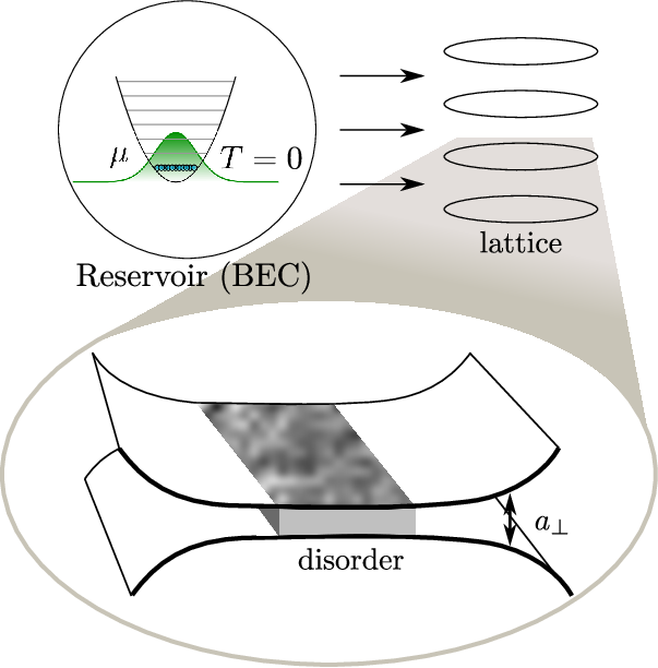
A many–body model for the description of such a quantum transport problem is given by a set of evolution equations for the field operator of the bosons in the scattering region, where is the spatial position, and for the particle annihilation operator of the source , whose evolution equations are given by Chrétien et al. 2019; Ernst et al. 2010
| (1) | ||||
| (2) |
In Eqs. (1) and (2), ) is the two–dimensional single–particle Hamiltonian describing the propagation of particles in the disorder potential , with the reduced Planck constant and the mass of the atoms. We also introduced the position–dependent coupling strength which couples the reservoir to the scattering region and , the effective interaction strength. In the presence of a 2D confinement, it is given by , with the 2D effective dimensionless interaction strength
| (3) |
where is the s–wave scattering length of the atoms under study and the oscillator length associated with the transverse confinement. Due to the spatial dependence of which follows the spatial profile of the confining potential, the interaction strength depends on the longitudinal propagation coordinate. We assume it to be adiabatically and smoothly ramped on from zero at position to a finite value at position and then ramped off from at position to zero at position , using a smooth switching function Hartmann 2014 represented in panel (e) of Fig. 2 whose profile (59) is detailed in Appendix B.
The reservoir is given by a trapped Bose–Einstein condensate filled with atoms. In order to ease the calculations, we choose an idealised profile for the coupling
| (4) |
which acts as a source that injects particles into the scattering plane at position , with a transverse profile that we assume to be homogeneous. The temporal profile of the coupling is adiabatically and smoothly ramped from zero to a constant value (this can be experimentally achieved by varying the intensity of the radio–frequency field in case of outcoupling via a radio–frequency knife Guerin et al. 2006) following the smooth switching function Hartmann 2014 profile (60) described in Appendix B. If this coupling tends to zero in such a manner that the product remains constant Guerin et al. 2006; Riou et al. 2008; Dujardin et al. 2014, then a stationary many–body scattering state can be realised.
The disorder potential we use in this paper is generated by
| (5) |
where the correlator is chosen as a Gaussian white noise satisfying as well as . This potential is such that its probability distribution to obtain a certain value for is given by the gaussian distribution.
| (6) |
The disorder potential in Eq. (5) is such that its average value vanishes (with the random average) and its two–point correlation function
| (7) |
is of Gaussian shape. Note that even though the Gaussian two point correlator is not identical to the one describing an optical speckle field, the predictions obtained with this disorder potential are nevertheless expected to be very similar to the ones that result from a speckle disorder, provided the disorder correlation lengths are identical Paul et al. 2009.
III Numerical methods
III.1 Discretisation procedure
In order to numerically implement the truncated Wigner method, we perform a discretisation of the 2D scattering region of length and width resulting in a series of sites labelled by and and spaced by the grid spacing . As is usually done in that case, we describe the kinetic energy operator in terms of a finite–difference scheme
| (8) | ||||
| (9) |
As a result of the finite–difference scheme discretisation, each site acquires both an on–site energy and a nearest–neighbour hopping term . The Hamiltonian resulting from the discretisation of space reads
| (10) |
where (resp. ) is the creation (resp. annihilation) operator at site and (resp. ) is the creation (resp. annihilation) operator of the source which is maintained at the chemical potential and vanishing temperature . We implement smooth exterior complex scaling in the longitudinal direction in order to absorb outgoing waves Balslev and Combes 1971; Barry 1973; Barry 1979; Junker 1982; Reinhardt 1982; Ho 1983; Löwdin 1988; Rom et al. 1990; Moiseyev 1998; Moiseyev and Cederbaum 2005; Dujardin et al. 2015a; Chrétien et al. 2019 and we consider periodic boundary conditions in the transverse direction.
The on–site interaction parameter is defined as
| (11) |
and is controlled by the dimensionless parameter . As Ref. Rontani et al. 2017 indicates, this choice for the on–site interaction parameter exhibits convergence issues in the formal limit . In Appendix C, we determine the correct scaling of this interaction parameter as a function of and conclude that for the choice we made, corrections to the scaling (11) are negligible.
In order to properly discretise the disorder potential, we discretise the distribution in the two–point correlation function of the correlator, which amounts to generating within the disordered slab complex Gaussian random numbers which fulfil
| (12) |
and satisfy the periodic boundary conditions . One has then to take the convolution product of those numbers with a Gaussian envelope so that the disorder at point is generated by
| (13) |
with the Gaussian weight
| (14) |
where is the disorder strength and its correlation length.
In the Heisenberg picture, the Hamiltonian provided in Eq. (10) yields the evolution of the annihilation operators according to
| (15) | ||||
| (16) |
In the absence of interaction and disorder, a steady many–body scattering state can be achieved. It is characterised by a stationary density and current that are given by Dujardin et al. 2015a; Dujardin et al. 2014; Chrétien et al. 2019
| (17) | ||||
| (18) |
III.2 Mean–field Gross–Pitaevskii approach
In the limit of a large atomic density and small interaction strength, the numerical integration of the Gross–Pitaevskii equation has revealed to provide very satisfactory descriptions in various atom–lasers scenarios Leboeuf and Pavloff 2001; Carusotto 2001; Paul et al. 2005a; Paul et al. 2005b; Paul et al. 2007. The principle of the mean–field approximation lies in the fact that quantum operators can be replaced by c–numbers as long as on-site densities are large and the interaction strength weak. In this approximation, and making the ansätze and , Eqs. (15) and (16) reduce to the discretised Gross–Pitaevskii equation
| (19) | ||||
| (20) |
with the initial conditions and , corresponding to an empty scattering region and a coherent Bose–Einstein condensate within the reservoir of atoms.
Inspecting Eq. (19) and (20), we can deduce that for some finite time interval , implying that in the formal limit where the coupling tends to zero in such a manner that remains constant11 1 This implies in practice that one would consider a large population of reservoir atoms (say, ) and a small outcoupling amplitude (say, in the natural units that we consider here) in such a way that the two compensate each other, giving rise to a finite product ., can be safely assumed to be constant in time, thereby yielding a nonlinear Schrödinger equation with a source term Paul et al. 2005a; Paul et al. 2007; Ernst et al. 2010 given by
| (21) | ||||
Here, an effective hopping term
| (22) |
is introduced to implement complex scaling where, within the scattering region, , leaving the Hamiltonian unchanged, whereas outside the scattering region is smoothly ramped to so that the coordinate is rotated in the complex plane according to , with the rotation angle Balslev and Combes 1971; Barry 1973; Barry 1979; Junker 1982; Reinhardt 1982; Ho 1983; Löwdin 1988; Rom et al. 1990; Moiseyev 1998; Moiseyev and Cederbaum 2005; Dujardin et al. 2015a; Chrétien et al. 2019. This rotation of the coordinate allows to absorb outgoing waves and hence to model open systems.
The approach developed here, which has been used in various situations Leboeuf and Pavloff 2001; Carusotto 2001; Paul et al. 2005a; Paul et al. 2005b; Paul et al. 2007, suffers from a major drawback. Because of two–body scattering Dujardin et al. 2016; Geiger et al. 2012; Geiger et al. 2013, a non–condensed population can be created as a result of a weak atom–atom interaction, particularly in the presence of disordered potentials. Those effects must be tackled by means of a method going beyond the mean–field approach.
III.3 Truncated Wigner method
The drawback related to the effects beyond the mean–field approach can be overcome with the truncated Wigner method Wigner 1931; Wigner 1932; Moyal 1949; Steel et al. 1998; Sinatra et al. 2002; Polkovnikov 2003, which has been successfully used in the context of atom–laser scenarios Dujardin et al. 2015a; Dujardin et al. 2015b. This method consists in finding a map between the von Neumann equation governing the time evolution of the density matrix of the system and the related Wigner function Wigner 1931; Wigner 1932 defined in the phase space spanned with the classical fields at sites . The resulting equation, containing third order derivatives of the classical fields , is practically impossible to integrate because of the prohibitively large dimension of the underlying phase space Dujardin et al. 2015a. The principle of the truncated Wigner method lies in the omission of those third–order derivative terms, hence resulting in a Fokker–Planck equation with a drift term. The former can be mapped to a set of coupled Langevin equations for the time–dependent canonically conjugated variables and , which we refer to as classical field amplitudes. The evolution equation is given by
| (23) |
with the function introduced in Eq. (22) for the implementation of complex scaling. The last line of Eq. (23) describes how the initial vacuum fluctuations outside the scattering region penetrate the system and represent quantum noise that enters the scattering region Dujardin et al. 2015a. It is given by
| (24) | ||||
| (25) |
with and
| (26) |
where are the Bessel functions of the first–kind of order and
| (27) |
We use classical field amplitudes that are randomly chosen to properly sample the initial many–body quantum state of the system. At initial time, the scattering region is fully empty and the corresponding Wigner function is a product of vacuum Wigner functions
| (28) |
The source of atoms is populated with a large number of atoms, which allows one to treat the source as a coherent state whose Wigner function reads
| (29) |
The Wigner function that describes the whole system is simply given by the product of the Wigner functions (28) and (29)
| (30) |
Consequently, the classical field amplitudes are chosen as
| (31) |
where and are real and independent gaussian random variables fulfilling
| (32) | ||||
| (33) | ||||
| (34) |
where denotes an average over the random variables. That choice for the classical field amplitudes implies that a fictious average vacuum population is artificially introduced at the initial time. The computation of the atomic density must therefore include a subtraction of this half fictitious particle per site.
Owing to the large number of atoms that populate the source, we can safely consider that the relative uncertainties of both the amplitude and the phase of the source are negligible. This approximation allows us to treat the source classically and to set . We additionally choose while keeping finite and constant, allowing us to neglect the source depletion and any back–action of the scattering region on the source Dujardin et al. 2015a. In this limit, one can solely focus on the evolution within the scattering region, and the propagation equation for the amplitude of the classical fields on each point of our lattice is therefore given by Eq. (23).
An average performed over the sampling of the initial many–body quantum state gives access to the observables of interest. We demonstrate this for the mode density in the momentum space which is evaluated in a slab of sites in the upstream region. This mode density is yielded as
| (35) |
where the subtraction of compensates for the artificial atom per site in the momentum space, as explained above. The truncated Wigner method allows one, contrarily to a mean–field approach, to access both coherent and incoherent quantities. The coherent contributions to the mode density in momentum space is given by
| (36) |
and the incoherent one is then obtained through
| (37) |
This notion of coherence is meaningful for matter waves and characterizes the capacity of the atom laser to produce superposition and interference effects. Note that the interaction–induced loss of this matter–wave coherence must not be confused with environment–induced decoherence in the many–body Fock space that would arise if the system is coupled to a heat bath.
IV Results
IV.1 Coherent backscattering peak
We first perform a mean–field study. Considering that initially the scattering region, depicted in panel (a) of Fig. 2, is totally empty, i.e. at , we numerically integrate Eq. (21) on the grid depicted in panel (b) of Fig. 2 for various disorder potentials and perform the disorder averages of the observables under study. The scattering geometry can be represented by a region of space where we consider the presence of a smooth gaussian correlated disorder as is described in Eq. (13) surrounded by two regions where , as depicted in panel (c) of Fig. 2. We also consider the presence of an effective interaction strength that is constant and equal to in the disordered region and that is adiabatically ramped from zero to upstream from the disordered slab and from to zero downstream, following the profile (e) of Fig. 2.

Provided the nonlinearity remains sufficiently small in the Gross–Pitaevskii equation (21), there exists a steady stable scattering state Johansson et al. 2009. At higher interaction strengths however, dynamical instabilities can occur Skipetrov and Maynard 2000; Paul et al. 2005b, thus rendering a steady scattering state unreachable because the scattering process remains always time–dependent. Since we want to focus on quasi–steady scattering processes, we have to restrict the interaction strength to very low values.
In the absence of nonlinearity, we can, for each disorder realisation, reach a steady scattering state, one of which being displayed in panel (d) of Fig. 2. Taking the disorder average of these states leads to the coherent mode and to the mean density , depending on whether the disorder average is performed before or after the square modulus. The lower right panel of Fig. 2 shows an average over the direction of and . We observe, as was also found in Hartung et al. 2008, an exponential decay of the coherent mode where is the scattering mean free path. From panel (f) of Fig. 2, we extract , indicating that we are in the so–called weak disorder regime, as well as in the diffusive regime, which is also confirmed by the linear decrease over the longitudinal direction of the density. This allows us to compute the Boltzmann mean free path which is defined as Akkermans and Montambaux 2007
| (38) |
where is the modified Bessel function of order , yielding . We also extract the transport mean free path Freund et al. 1988 using the scaling of the disorder–averaged density and find , indicating that the chosen correlation length yields anisotropic scattering. Finally, the localisation length is provided by Kuhn et al. 2007 and exceeds, by far, the dimension of the scattering region.
The two–dimensional Fourier transform of the wavefunction is taken in an upstream region where both disorder and nonlinearity are equal to zero. The different Fourier modes can hence be associated to outgoing waves in various directions with the wavenumbers , describing the propagation in a spatial direction characterised by the angle , with .

In the absence of interaction, Gross–Pitaevskii simulations show the appearance of coherent backscattering. This is clearly visible in the panel (a) of Fig. 3, where we observe that the modes associated to outgoing waves display similar populations, forming a ridge along the circle , which indicates that all directions of reflection are approximately equivalently populated. The inset of panel (a) of Fig. 3 shows a zoom around , corresponding to the backscattered direction, which highlights a higher population of the mode associated with coherent backscattering, as compared to other scattering directions. Artificial oscillations, which are the result of the periodic boundary conditions, are present for large angles, indicating that a more suitable method to extract and analyse coherent backscattering is required.
The heigth of the CBS peak in Fig. 3(a) is reduced compared to the semiclassical expectation of a factor 2 enhancement. This reduction is due to the presence of short length self–retracing paths, mainly those that feature a backreflection at only a single scattering event within the disordered region. Those paths are identical to their time–reversed counterpart and bring no contribution to CBS. Their relative weight in the sum over all backreflected paths gives therefore rise to a reduction of the CBS enhancement.
It has been argued in Ref. Hartmann et al. 2012 that this reduction of the CBS peak height, induced by self–retracing paths, should be quantitatively identical to the depth of the dip that forms in the presence of mean–field interaction. The occurrence of this dip is shown in Fig. 3(b) which displays that the CBS peak becomes a pronounced dip in the presence of interaction, as was also observed in Refs. Hartung et al. 2008. Beyond the mean–field regime, truncated Wigner simulations depicted in panel (c) indicate that this inversion prevails. It is however partially destroyed due to many–body interaction effects that create incoherent particles, from which results dephasing.
Despite the fact that the Truncated Wigner method accounts for off–shell scattering events between the atoms Dujardin et al. 2015a, which populate states with a kinetic energy different from that of the incident particles, we do not observe a significant broadening of the density distribution about the energy shell in the presence of interaction Geiger et al. 2013. We attribute this to the fact that the atoms do not stay long in the disordered region where they interact. This thermal cloud around the condensate is expected to be more pronounced in a turbulent regime which we do not study here. As a matter of fact, the set of parameters chosen in Fig. 3(c) yields a mostly coherent current, as is confirmed in Fig. 5(c).
IV.2 Angular resolved current
The drawback of the two–dimensional Fourier transform is that it demands a large number of sites to yield a satisfactory resolution. An alternative way to extract the reflected part of the wavefunction is to take the partial Fourier transform of along the y–direction. This new wavefunction contains both the incident part () and the reflected part () and one should get rid of the former. Considering at position and position , we have, introducing , the amplitudes of the incident and reflected waves
| (39) |
whose solution is found to be
| (40) |
This allows us to separate the incoming and reflected components of the wavefunction at position , the latter being given by
| (41) |
The current density in the direction is given by
| (42) |
where we have written and . We finally note that and must be chosen in a region where the interaction (and consequently the disorder) is equal to zero. This allows us to apply the superposition principle and to associate the Fourier modes in Eq. (42) to directions in the two–dimensional space. In the following, we choose and .

The angular resolved current is depicted in Fig. 4 for different values of the interaction strength . In the noninteracting case, we recover the characteristic coherent backscattering peak we already observed in the inset of Fig. 3 (a). For higher interaction strengths, the peak turns to a dip, as was also observed in Ref. Hartung et al. 2008, indicating a crossover from constructive to destructive interferences. Considering a tilt of the source by an angle , which amounts to choosing the tilted profile in Eq. (4), the inset of Fig. 4 shows that the coherent backscattering peak and the related inversion are realised in the exact opposite direction. This confirms the interference effect between scattering paths and their time–reversed counterparts and validates that coherent backscattering is the underlying mechanism.
IV.3 Inversion of coherent backscattering beyond the mean–field regime
While it is already explained in Sec. III.3, namely in Eqs. (35), (36) and (37), how to compute the total, coherent and incoherent mode densities in the momentum space, the procedure for doing so for the current requires further explanations. Depending on whether the average is performed over the wavefunctions (the square modulus being taken on the average wavefunction) or over the square modulus of those, one can define total and coherent current, similarly as for the Gross–Pitaevskii simulations
| (43) | ||||
| (44) |
The incoherent part of the current is obtained by subtracting the coherent contribution from the total one
| (45) |
This allows us to investigate to which extent the inverted structure is due to coherent contribution, and to find out which interaction strength leads to a dephasing between interfering trajectories and finally yields a structureless current, with a dominant incoherent contribution, as was predicted by a nonlinear diagrammatic theory in Geiger et al. 2013 and numerically confirmed in Chrétien et al. 2019 for Al’tshuler–Aronov–Spivak oscillations (see also Ref. Scott and Hutchinson 2008 in this context). The identification of this dephasing regime is fundamental, as it provides information whether the effect is experimentally observable.
We first perform truncated Wigner simulations for the case of a partial inversion of coherent backscattering that corresponds to the red (dark grey) curve of Fig. 4, that is, a scenario with . We vary both the density per unit surface and the interaction strength while maintaining the nonlinearity constant, which allows us to explore the many–body effects beyond the mean–field regime. Fig. 5 shows that a partial inversion of coherent backscattering prevails beyond the mean–field regime. Panel (f) of Fig. 5 indeed indicates that even for densities as low as , the inversion is still preserved, although a certain dephasing has already appeared, thereby partially destroying the effect.
We now evaluate whether this effect is observable with 87Rb. Considering the 2D interaction strength which we can write as
| (46) |
with the oscillator length associated to the confinement frequency of the trap, we can write within the disordered region
| (47) |
In the simulations, we have the chemical potential , corresponding to with the velocity of the injected particles. In the case we investigate here, where , the injected density is found to be
| (48) |
and essentially depends on the s–wave scattering length and the oscillator length which scales as . Considering the s–wave scattering length m of 87Rb and its mass kg, we find that for a confinement frequency of Hz, the injected density reaches . This corresponds to a situation similar as that depicted in the panel (e) of Fig. 5. We therefore believe that such an inversion of coherent backscattering should be observable experimentally.
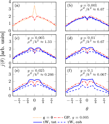
We also note that we have to enforce in order to safely neglect the excitation of the transverse modes of the condensates. With the parameters we used, the choice of a velocity for the injected particles of m/s satisfies this constraint. We should note that one would still be in a supersonic regime with such a velocity. Indeed, the speed of the sound within the condensate is given by , where the factor comes from the transverse wavefunction in its ground state evaluated for and where is the 3D interaction strength. This allows us to rewrite the speed of sound within the condensate as , which yields for parameters used in Fig. 5 and Fig. 6. This confirms that an inversion of coherent backscattering might be observed with 87Rb.
Fig. 6 is dedicated to a truncated Wigner study of the regime corresponding to a full inversion of coherent backscattering. As could be inferred from Fig. 5, the dephasing regime is reached with higher nonlinearities. As panel (f) indicates, the coherent contribution carrying the inverted dip is now hidden behind a flat and structureless incoherent contribution that overshadows the signature of interference and interaction. Conducting the same reasoning as for Fig. 5 with a nonlinearity equal to leads to an injected density , which corresponds to a situation intermediate between those depicted in the panels (d) and (e) of Fig. 6. Pushing the system further in the quantum limit by increasing the interaction strength and decreasing accordingly the injected density induces, however, dephasing, as panel (f) indicates, where the coherent inversion of backscattering is drowned by an incoherent contribution.

V Conclusions
In conclusion, we numerically studied the two–dimensional transport of Bose–Einstein condensates across a disordered region, which gives rise to a weak–localisation scenario that occurs through coherent backscattering. In the mean–field regime, which is studied by means of the Gross–Pitaevskii equation, the presence of an atom–atom interaction gives rise to a crossover around from constructive to destructive interference, the peak in the backscattered current becoming a pronounced dip, thereby reverting weak localisation Hartung et al. 2008; Hartmann et al. 2012. Truncated Wigner simulations show that the coherent backscattering inversion is also encountered when accounting for effects beyond the mean–field approximation. As was observed in Refs. Chrétien et al. 2019; Geiger et al. 2013 when pushing the limit far beyond the mean–field regime, quantum interference effects face dephasing, and the dip structure is completely overshadowed by a dominant incoherent contribution.
We believe that this effect is experimentally observable for 87Rb. We indeed found for experimentally realistic parameters a value for the injected density, namely for which the inversion is predicted to be still observable. Other species, such as 39K, whose s–wave scattering length can be tuned by means of Feshbach resonances to very low values, are also good candidates to realise a full inversion of coherent backscattering.
The present study had a clear focus on the inversion of the CBS peak in the framework of a quasi–stationary 2D propagation of a Bose–Einstein condensate across a disordered region. It thereby left out a number of interesting side investigations that one could have performed in this context with our numerical setup. Among these are the study of wavepacket propagation processes across the disorder potential, in alignement with the experiments of Ref. Jendrzejewski et al. 2012 (see also Valdes and Wellens 2016), as well as coherent forward scattering Karpiuk et al. 2012; Ghosh et al. 2014; Lee et al. 2014; Micklitz et al. 2014; Valdes and Wellens 2016 which is expected to occur in the downstream region behind the disordered slab. A comparison with the study undertaken in Ref. Skipetrov et al. 2008, dedicated to the expansion of a –resolved source where it is argued that as the cloud expands for a sufficiently long time interaction disappears, would also be relevant. Furthermore, this study lacks a quantitative comparison with diagrammatic many–body scattering theory Geiger et al. 2013, which is, however, difficult to carry out because of the inhonomegenous density profile of the Bose–Einstein condensate. In that context, it would therefore be interesting to investigate the transport of Bose–Einstein condensates through 2D billiard potentials Hartmann et al. 2012 or in the non-equilibrium configuration described in Ref. Scoquart et al. 2020, where a homogeneous density profile is expected.
Acknowledgements.
The computational resources have been provided by the Consortium des Equipements de Calcul Intensif (CÉCI), funded by the F.R.S.-FNRS under Grant No. 2.5020.11.Appendix A Numerical scheme
The discretisation scheme of the partial differential equations in terms of finite differences naturally results in a set of ordinary differential equations which we numerically integrate. For that purpose, we use a very general numerical scheme based on the expansion of the solution in a Taylor series Meyer 1986. This method allows in principle to determine the solution of every ordinary differential equation, but requires on the other hand to compute the derivatives up to the desired order, which may be tedious and inefficient in some cases. Automatic differention techniques Wengert 1964; Barton et al. 1971; Bartholomew-Biggs et al. 2000; Bücker et al. 2006; Naumann 2012 may be envisaged to circumvent this major drawback. Knowing the solution of the differential equation at time , it is obtained at time using the expansion
| (49) |
that should be repeated iteratively from until reaching . Following this principle, the discrete wavefunction at site is expanded in Taylor series and is therefore written at time as
| (50) |
and will be propagated from initial time to final time by means of this equation. In Eq. (50), denotes the maximal order considered for the derivative in the Taylor expansion. This expansion requires that we are able to compute the derivatives of up to order which is readily achieved by differentiating the field equations (23) which gives, for instance, for the second time derivative
| (51) |
where denotes the derivatives with respect to and where we have omitted the derivative of the source term because we assume that the coupling varies so slowly that its derivative with respect to is negligible.
While derivatives of the wavefunction are easily found iteratively, the derivatives of the nonlinear term as well as that of the noise terms are more complicated to obtain. Exploiting the property
| (52) |
where is the trinomial coefficient, the derivative of the nonlinear term reads
| (53) |
One also has to compute the derivative of the noise terms in Eqs. (24) and (25). Noting that the writing of those terms suggests that an inverse discrete Fourier transform has been performed, one can compute the time derivative of the Fourier coefficients of the noise term
| (54) |
which turn out to be
| (55) | ||||
| (56) |
once again involving , the trinomial coefficient, as well as time derivatives of in the longitudinal direction and in the transverse direction. In Eq. (55) and (56), denotes the initial condition for the wavefunction, which in the mean–field approximation, is identically equal to zero, thereby yielding , for all . In the truncated Wigner context, however, we have seen that those classical fields are sampled as prescribed in Sec. III.3, with a different sampling from one realisation of the initial condition to another, the convolution kernel remaining unchanged.
Appendix B A smooth switching function
The purpose of this Appendix is to present the smooth switching function that we use in this work, which was derived by Hartmann Hartmann 2014. Considering an interval , we are looking for a function that is exactly zero farther than from the interval and that smoothly reaches over that distance within the interval, as is shown in Fig. 7.

We start by defining the auxiliary test function
| (57) |
where and are numerical parameters that are chosen so that is as smooth as possible. Based on this test function, we build the function which is defined as
| (58) |
The smooth switching function describing describing the spatial profile of the interaction is then defined as
| (59) |
The smooth switching function describing the ramping of the source is given by
| (60) |
Specifically, we choose for a smooth ramping and typically obtain a stationary scattering state after .
Appendix C Effective atom–atom interaction strength on the square lattice
In this appendix we discuss how to properly choose the interaction parameter on the numerical grid that we introduced in order to implement the Truncated Wigner method. As each grid point covers a square of the area , with the lattice spacing, it appears most natural to define the on–site interaction parameter as
| (61) |
where is the effective two-dimensional atom-atom interaction strength, assuming that the atomic cloud is located in the transverse ground state of the 2D confinement, and denotes its dimensionless counterpart defined according to Eq. (3). This naïve choice, which is retained within Eqs. (10), (15), (19) and (23) for the sake of simplicity, is problematic insofar as it exhibits convergence issues in the formal limit , as was discussed in detail in Ref. Rontani et al. 2017.
To determine the correct scaling of the on–site interaction parameter with the grid spacing, it is useful to study a two–body scattering problem on the chosen numerical grid and compare the outcome of this study with the solution of this problem in the continuous 2D space, which was obtained in Refs. Petrov et al. 2000; Petrov and Shlyapnikov 2001. Considering a harmonic confinement potential with the frequency in the transverse direction, the Hamiltonian describing this two–body system in the full three–dimensional space reads
| (62) |
with the position coordinates of the atom no. and the two–body interaction strength. As the latter depends only on the distance between the two atoms, it is useful to separate the center–of–mass and relative coordinates of the two atoms and thereby map the collision process between the two atoms into an effective one–body scattering problem in the relative coordinates. The exact solution of the latter in continuous space can then be compared with the analytic solution of the analogous scattering problem in the presence of a square–lattice discretization of the in–plane relative coordinates.
We should keep in mind, however, that the latter is not exactly equivalent to the original discretization procedure carried out in the individual in–plane coordinates and of the atoms, which is effectively employed for our numerical simulations. Indeed, the conventional transformation to the center–of–mass coordinates and relative coordinates maps squares into non–equilateral rectangles and therefore does not preserve the spacing scales of the discretization procedure. An approximate equivalence of the two square–lattice discretizations can nevertheless be established by redefining the new coordinates and in a more symmetric manner, namely through
| (63) | |||||
| (64) |
which corresponds to a unitary mapping that preserves the shape of the lattice squares resulting from the discretization. We therefore adopt this latter symmetric definition of “center–of–mass” and “relative” coordinates in the following. The Hamiltonian (62) can then be separated as with the Hamiltonians
| (65) | |||||
| (66) |
that govern the dynamics in the center–of–mass and relative coordinates, respectively.
The interaction is modeled via the Fermi–Huang pseudopotential
| (67) |
with
| (68) |
where is the –wave scattering length of the atoms. The expression (67) can be seen as an augmented version of Dirac’s delta distribution which is designed such that it can deal with singularities in the wave function. We can therefore formally express the Hamiltonian (66) describing the relative motion as
| (69) |
where we define by
| (70) |
the noninteracting part of the Hamiltonian and by the projector onto the origin in position space, corresponding to the augmented delta function defined above. Noting that according to Eq. (67), we obtain .
Owing to the rank–one nature of the perturbation operator in the expression (69) for the Hamiltonian, the Lippmann–Schwinger equation describing the scattering process in the relative coordinates can be formally solved in terms of the noninteracting retarded Green operator . More specifically, we obtain for the full retarded Green operator the explicit expression
| (71) |
Its matrix elements in the position representation read
| (72) | ||||
for , , and , where we use the fact that the noninteracting Green function is well–behaved and does not feature any singularity for .
The projection of the matrix elements (72) to the 2D plane to which the atoms are confined gives rise to the equation
| (73) | ||||
where we define by the 2D position eigenstate on the plane, which is anchored on the normalized ground state wavefunction of the transverse confinement potential. Quite straightforwardly, we evaluate
| (74) |
as well as
| (75) |
with the Hankel function of the first kind of order zero and
| (76) |
the in–plane wave number associated with the energy . The denominator appearing on the right–hand side of Eq. (73) was calculated in Refs. Petrov et al. 2000 and Petrov and Shlyapnikov 2001, Assuming that the in–plane kinetic energy of the atoms is much smaller than the transverse confinement energy , such that a population of transversally excited modes is energetically suppressed, this calculation yields
| (77) |
with the numerical constant Petrov and Shlyapnikov 2001. Combining Eqs. (68), (73), (74), (75), and (77), we altogether obtain
| (78) | ||||
for the in–plane position representation of the Green function. Note that this expression is valid in leading order in . Corrections scaling linearly with will arise as soon as the in–plane kinetic energy of the atoms becomes comparable with the transverse excitation energy .
Let us now redo this calculation of the Green function for a square–lattice discretization of the two–dimensional in–plane space with the grid spacing . Using the finite–difference scheme (8) and (9), we model the projection of the noninteracting part (70) of the Hamiltonian to the transverse ground mode as
| (79) |
where we define by the localized lattice site orbitals satisfying and by the characteristic energy scale of the lattice. The interaction operator is modeled by a projector onto the origin site of this lattice according to
| (80) |
represents the interaction parameter that one would use in a square–lattice model for the original two–body Hamiltonian (62) with the same grid spacing , where the interaction operator would read
| (81) |
Since this expression is supposed to model the effect of a two–dimensional
delta function and since, as is seen in Eq. (66), the prefactor
has to accounted for in the argument of this function when
transforming from the original particle coordinates to the symmetric
center–of–mass and relative coordinates (63) and (64),
we obtain the prefactor in the expression (80) for the
interaction operator in the relative coordinates.
Since we can write the total lattice Hamiltonian of the relative motion projected onto the transverse ground mode as
| (82) |
its associated Green operator is, according to Eq. (71), explicitly expressed as
| (83) |
in terms of the noninteracting Green operator . The latter is calculated via a diagonalization of the noninteracting lattice Hamiltonian (79) according to
| (84) |
with the normalized two–dimensional plane–wave eigenstates being defined by
| (85) |
In the continuous limit , which is taken such that is kept finite, we obtain
| (86) |
in perfect analogy with Eq. (74), where we formally define .
The diagonal matrix element of the noninteracting Green operator on the origin site is determined as
| (87) |
Defining
| (88) |
with the property in the continuous limit 22 2 Strictly speaking, this property is not satisfied in the numerical simulations the results of which are presented in this article, where for the sake of numerical efficiency we chose , which would correspond to . Numerical convergence checks were performed through comparisons with some test calculations that were carried out for (slightly) lower values of ., where we use the definition (76) of the in–plane wave number associated with the energy , we obtain through standard residue calculus
| (89) |
Evaluating separately
| (90) | |||||
| (91) |
yields the expression
| (92) |
in the continuous limit.
Inserting this expression and Eq. (86) into the expression (83) for the Green operator yields its matrix elements as
| (93) |
Comparing this expression with the analogous matrix elements (78) of the spatially continuous Green function finally yields the prescription that we have to choose the square–lattice interaction parameter as
| (94) |
as a function of the grid spacing in order to obtain a match between the expressions (78) and (93) for the continuous and discretized Green functions.
In the numerical practice of our calculations, we chose not too fine grids in order to limit the numerical effort. Consequently, the logarithmic correction arising in the denominator of Eq. (94) can safely be neglected. Most specifically, for the choice of the grid spacing and the inverse wave number, we obtain , while we have for 87Rb in the presence of the transverse confinement frequency Hz. This justifies the usage of the “naïve” expression (61) for the interaction parameter in our numerical simulations.
References
- Wolf and Maret (1985) P.-E. Wolf and G. Maret, Phys. Rev. Lett. 55, 2696 (1985).
- Wolf, P.E. et al. (1988) Wolf, P.E., Maret, G., Akkermans, E., and Maynard, R., J. Phys. France 49, 63 (1988).
- Akkermans, E. et al. (1988) Akkermans, E., Wolf, P.E., Maynard, R., and Maret, G., J. Phys. France 49, 77 (1988).
- Van Albada and Lagendijk (1985) M. P. Van Albada and A. Lagendijk, Phys. Rev. Lett. 55, 2692 (1985).
- Hapke (2002) B. Hapke, Icarus 157, 523 (2002).
- Margerin et al. (2009) L. Margerin, M. Campillo, B. A. Van Tiggelen, and R. Hennino, Geophysical Journal International 177, 571 (2009).
- Wiersma et al. (1995) D. S. Wiersma, M. P. van Albada, B. A. van Tiggelen, and A. Lagendijk, Phys. Rev. Lett. 74, 4193 (1995).
- de Rosny et al. (2000) J. de Rosny, A. Tourin, and M. Fink, Phys. Rev. Lett. 84, 1693 (2000).
- Tourin et al. (1997) A. Tourin, A. Derode, P. Roux, B. A. van Tiggelen, and M. Fink, Phys. Rev. Lett. 79, 3637 (1997).
- Jendrzejewski et al. (2012) F. Jendrzejewski, K. Müller, J. Richard, A. Date, T. Plisson, P. Bouyer, A. Aspect, and V. Josse, Phys. Rev. Lett. 109, 195302 (2012).
- Altshuler et al. (1980) B. L. Altshuler, D. Khmel’nitzkii, A. I. Larkin, and P. A. Lee, Phys. Rev. B 22, 5142 (1980).
- Bergmann (1984) G. Bergmann, Physics Reports 107, 1 (1984).
- Engl et al. (2014) T. Engl, J. Dujardin, A. Argüelles, P. Schlagheck, K. Richter, and J.-D. Urbina, Phys. Rev. Lett. 112, 140403 (2014).
- Engl et al. (2018) T. Engl, J. D. Urbina, K. Richter, and P. Schlagheck, Phys. Rev. A 98, 013630 (2018).
- Anderson (1958) P. W. Anderson, Phys. Rev. 109, 1492 (1958).
- Vollhardt and Wölfle (1980) D. Vollhardt and P. Wölfle, Phys. Rev. B 22, 4666 (1980).
- Karpiuk et al. (2012) T. Karpiuk, N. Cherroret, K. L. Lee, B. Grémaud, C. A. Müller, and C. Miniatura, Phys. Rev. Lett. 109, 190601 (2012).
- Ghosh et al. (2014) S. Ghosh, N. Cherroret, B. Grémaud, C. Miniatura, and D. Delande, Phys. Rev. A 90, 063602 (2014).
- Lee et al. (2014) K. L. Lee, B. Grémaud, and C. Miniatura, Phys. Rev. A 90, 043605 (2014).
- Micklitz et al. (2014) T. Micklitz, C. A. Müller, and A. Altland, Phys. Rev. Lett. 112, 110602 (2014).
- Valdes and Wellens (2016) J. P. R. Valdes and T. Wellens, Phys. Rev. A 93, 063634 (2016).
- Wellens and Grémaud (2008) T. Wellens and B. Grémaud, Phys. Rev. Lett. 100, 033902 (2008).
- Finlayson and Stegeman (1990) N. Finlayson and G. I. Stegeman, Appl. Phys. Lett. 56, 2276 (1990).
- Hennig and Tsironis (1999) D. Hennig and G. Tsironis, Physics Reports 307, 333 (1999).
- Agranovich and Kravtsov (1991) V. M. Agranovich and V. E. Kravtsov, Phys. Rev. B 43, 13691 (1991).
- Hartung et al. (2008) M. Hartung, T. Wellens, C. A. Müller, K. Richter, and P. Schlagheck, Phys. Rev. Lett. 101, 020603 (2008).
- Hartmann et al. (2012) T. Hartmann, J. Michl, C. Petitjean, T. Wellens, J.-D. Urbina, K. Richter, and P. Schlagheck, Ann. Phys. 327, 1998 (2012).
- Chrétien et al. (2019) R. Chrétien, J. Rammensee, J. Dujardin, C. Petitjean, and P. Schlagheck, Phys. Rev. A 100, 033606 (2019).
- Geiger et al. (2013) T. Geiger, A. Buchleitner, and T. Wellens, New J. Phys. 15, 115015 (2013).
- Scoquart et al. (2020) T. Scoquart, T. Wellens, D. Delande, and N. Cherroret, Phys. Rev. Research 2, 033349 (2020).
- Wigner (1931) E. Wigner, Gruppentheorie und ihre Anwendung auf die Quantenmechanik der Atomspektren (Vieweg+Teubner Verlag, Wiesbaden, 1931).
- Wigner (1932) E. Wigner, Phys. Rev. 40, 749 (1932).
- Moyal (1949) J. E. Moyal, Proc. Cambridge Phil. Soc. 45, 99 (1949).
- Steel et al. (1998) M. J. Steel, M. K. Olsen, L. I. Plimak, P. D. Drummond, S. M. Tan, M. J. Collett, D. F. Walls, and R. Graham, Phys. Rev. A 58, 4824 (1998).
- Sinatra et al. (2002) A. Sinatra, C. Lobo, and Y. Castin, J. Phys. B 35, 3599 (2002).
- Polkovnikov (2003) A. Polkovnikov, Phys. Rev. A 68, 053604 (2003).
- Scott and Hutchinson (2008) R. G. Scott and D. A. W. Hutchinson, Phys. Rev. A 78, 063614 (2008).
- Dujardin et al. (2015a) J. Dujardin, A. Argüelles, and P. Schlagheck, Phys. Rev. A 91, 033614 (2015a).
- Dujardin et al. (2015b) J. Dujardin, T. Engl, J. D. Urbina, and P. Schlagheck, Annalen der Physik 527, 629 (2015b).
- Dujardin et al. (2016) J. Dujardin, T. Engl, and P. Schlagheck, Phys. Rev. A 93, 013612 (2016).
- Bloch et al. (1999) I. Bloch, T. W. Hänsch, and T. Esslinger, Phys. Rev. Lett. 82, 3008 (1999).
- Guerin et al. (2006) W. Guerin, J.-F. Riou, J. P. Gaebler, V. Josse, P. Bouyer, and A. Aspect, Phys. Rev. Lett. 97, 200402 (2006).
- Couvert et al. (2008) A. Couvert, M. Jeppesen, T. Kawalec, G. Reinaudi, R. Mathevet, and D. Guéry-Odelin, Europhys. Lett. 83, 50001 (2008), 0802.2601 .
- Gattobigio et al. (2009) G. L. Gattobigio, A. Couvert, M. Jeppesen, R. Mathevet, and D. Guéry-Odelin, Phys. Rev. A 80, 041605 (2009).
- Gattobigio et al. (2011) G. L. Gattobigio, A. Couvert, B. Georgeot, and D. Guéry-Odelin, Phys. Rev. Lett. 107, 254104 (2011).
- Vermersch et al. (2011) F. Vermersch, C. M. Fabre, P. Cheiney, G. L. Gattobigio, R. Mathevet, and D. Guéry-Odelin, Phys. Rev. A 84, 043618 (2011).
- Bolpasi et al. (2014) V. Bolpasi, N. K. Efremidis, M. J. Morrissey, P. C. Condylis, D. Sahagun, M. Baker, and W. von Klitzing, New J. Phys. 16, 033036 (2014).
- Lye et al. (2005) J. E. Lye, L. Fallani, M. Modugno, D. S. Wiersma, C. Fort, and M. Inguscio, Phys. Rev. Lett. 95, 070401 (2005).
- Ernst et al. (2010) T. Ernst, T. Paul, and P. Schlagheck, Phys. Rev. A 81, 013631 (2010).
- Hartmann (2014) T. Hartmann, Transport of Bose-Einstein condensates through two dimensional cavities, Ph.D. thesis, Universität Regensburg (2014).
- Riou et al. (2008) J.-F. Riou, Y. Le Coq, F. Impens, W. Guerin, C. J. Bordé, A. Aspect, and P. Bouyer, Phys. Rev. A 77, 033630 (2008).
- Dujardin et al. (2014) J. Dujardin, A. Saenz, and P. Schlagheck, Appl. Phys. B 117, 765 (2014).
- Paul et al. (2009) T. Paul, M. Albert, P. Schlagheck, P. Leboeuf, and N. Pavloff, Phys. Rev. A 80, 033615 (2009).
- Balslev and Combes (1971) E. Balslev and J. Combes, Commun. Math. Phys. 22, 280 (1971).
- Barry (1973) S. Barry, Ann. Math. 97, 247 (1973).
- Barry (1979) S. Barry, Phys. Lett. A 71, 211 (1979).
- Junker (1982) B. Junker, Adv. Atom. Mol. Phys. 18, 207 (1982).
- Reinhardt (1982) W. P. Reinhardt, Annu. Rev. Phys. Chem. 33, 223 (1982).
- Ho (1983) Y. Ho, Phys. Rep. 99, 1 (1983).
- Löwdin (1988) P.-O. Löwdin, Adv. Quant. Chem. 19, 87 (1988).
- Rom et al. (1990) N. Rom, E. Engdahl, and N. Moiseyev, J. Chem. Phys. 93, 3413 (1990).
- Moiseyev (1998) N. Moiseyev, Phys. Rep. 302, 212 (1998).
- Moiseyev and Cederbaum (2005) N. Moiseyev and L. S. Cederbaum, Phys. Rev. A 72, 33605 (2005).
- Rontani et al. (2017) M. Rontani, G. Eriksson, S. Åberg, and S. M. Reimann, J. Phys. B: At. Mol. Opt. Phys. 50, 065301 (2017).
- Leboeuf and Pavloff (2001) P. Leboeuf and N. Pavloff, Phys. Rev. A 64, 033602 (2001).
- Carusotto (2001) I. Carusotto, Phys. Rev. A 63, 023610 (2001).
- Paul et al. (2005a) T. Paul, K. Richter, and P. Schlagheck, Phys. Rev. Lett. 94, 020404 (2005a).
- Paul et al. (2005b) T. Paul, P. Leboeuf, N. Pavloff, K. Richter, and P. Schlagheck, Phys. Rev. A 72, 063621 (2005b).
- Paul et al. (2007) T. Paul, M. Hartung, K. Richter, and P. Schlagheck, Phys. Rev. A 76, 063605 (2007).
- (70) This implies in practice that one would consider a large population of reservoir atoms (say, ) and a small outcoupling amplitude (say, in the natural units that we consider here) in such a way that the two compensate each other, giving rise to a finite product .
- Geiger et al. (2012) T. Geiger, T. Wellens, and A. Buchleitner, Phys. Rev. Lett. 109, 030601 (2012).
- Johansson et al. (2009) M. Johansson, G. Kopidakis, S. Lepri, and S. Aubry, EPL (Europhysics Letters) 86, 10009 (2009).
- Skipetrov and Maynard (2000) S. E. Skipetrov and R. Maynard, Phys. Rev. Lett. 85, 736 (2000).
- Akkermans and Montambaux (2007) E. Akkermans and G. Montambaux, Mesoscopic Physics of Electrons and Photons (Cambridge University Press, 2007).
- Freund et al. (1988) I. Freund, M. Rosenbluh, R. Berkovits, and M. Kaveh, Phys. Rev. Lett. 61, 1214 (1988).
- Kuhn et al. (2007) R. C. Kuhn, O. Sigwarth, C. Miniatura, D. Delande, and C. A. Müller, New Journal of Physics 9, 161 (2007).
- Skipetrov et al. (2008) S. E. Skipetrov, A. Minguzzi, B. A. van Tiggelen, and B. Shapiro, Phys. Rev. Lett. 100, 165301 (2008).
- Meyer (1986) H.-D. Meyer, The Journal of Chemical Physics 84, 3147 (1986).
- Wengert (1964) R. E. Wengert, Commun. ACM 7, 463–464 (1964).
- Barton et al. (1971) D. Barton, I. M. Willers, and R. V. M. Zahar, in Mathematical Software, edited by J. Rice (Academic Press, New York, 1971) pp. 369–390.
- Bartholomew-Biggs et al. (2000) M. Bartholomew-Biggs, S. Brown, B. Christianson, and L. Dixon, Journal of Computational and Applied Mathematics 124, 171 (2000), numerical Analysis 2000. Vol. IV: Optimization and Nonlinear Equations.
- Bücker et al. (2006) M. Bücker, G. Corliss, P. Hovland, U. Naumann, and B. Norris, Automatic Differentiation: Applications, Theory, and Implementations (Lecture Notes in Computational Science and Engineering) (Springer-Verlag, Berlin, Heidelberg, 2006).
- Naumann (2012) U. Naumann, The Art of Differentiating Computer Programs: An Introduction to Algorithmic Differentiation (Society for Industrial and Applied Mathematics, USA, 2012).
- Petrov et al. (2000) D. S. Petrov, M. Holzmann, and G. V. Shlyapnikov, Phys. Rev. Lett. 84, 2551 (2000).
- Petrov and Shlyapnikov (2001) D. S. Petrov and G. V. Shlyapnikov, Phys. Rev. A 64, 012706 (2001).
- (86) Strictly speaking, this property is not satisfied in the numerical simulations the results of which are presented in this article, where for the sake of numerical efficiency we chose , which would correspond to . Numerical convergence checks were performed through comparisons with some test calculations that were carried out for (slightly) lower values of .