Skew-symmetric endomorphisms in : A unified canonical form with applications to conformal geometry
Abstract
We show the existence of families of orthonormal, future directed bases which allow to cast every skew-symmetric endomorphism of () in a single canonical form depending on a minimal number of parameters. This canonical form is shared by every pair of elements in differing by an orthochronous Lorentz transformation, i.e. it defines the orbits of the orthochronous Lorentz group under the adjoint action on its algebra. Using this form, we obtain the quotient topology of . From known relations between and the conformal Killing vector fields (CKVFs) of the sphere , a canonical form for CKVFs follows immediately. This form is used to find adapted coordinates to an arbitrary CKVF that covers all cases at the same time. We do the calculation for even and obtain the case of odd as a consequence. Finally, we employ the adapted coordinates to obtain a wide class of TT-tensors for , which provide Cauchy data at conformally flat null infinity . Specifically, this class of data is characterized for generating -vacuum spacetimes with two-symmetries, one of which axial, admitting a conformally flat . The class of data is infinite dimensional, depending on two arbitrary functions of one variable as well as a number of constants. Moreover, it contains the data for the Kerr-de Sitter spacetime, which we explicitly identify within.
1 Introduction
Having a Lie group acting on a space respresenting a set of physical quantities is always a desirable feature in a physical problem, as Lie groups represent symmetries (either global or gauge) and their presence is often translated into a simplification of the formal aspects of the problem. Roughly speaking, in this situation the “relevant” part for the physics effectively happens in the quotient space . For the study of these quotient spaces, one may be interested in obtaining a unified form to give a representative for every orbit in , i.e. a canonical form (also known as normal form). A particularly relevant case is when is a Lie algebra and its Lie group acting by the adjoint action, in which case the orbits are also called conjugacy classes of (see e.g. [5]). In the first part of this paper, we study the conjugacy classes of the pseudo-orthogonal group (or Lorentz group), for which we will obtain a canonical form. Our main interest on this, addressed in the second part of the paper, lies in its relation with the Cauchy problem of general relativity (GR) (cf. [11] and e.g. [7], [14]) and more precisely, its formulation at null infinity for the case of positive cosmological constant (cf. [12], [13]). In the remainder of this introduction we summarize our ideas and results, and we will also briefly review some results on conjugacy classes of Lie groups related to our case, as well as the Cauchy problem of GR with positive .
A typical example of a canonical form in the context described above, is the well-known Jordan form, which represents the conjugacy classes of (where is usually or the quaternions ). Besides this example, the problem of finding a canonical representative for the conjugacy classes of a Lie group has been adressed numerous times in the literature. The reader may find a list of canonical forms for algebras whose groups leave invariant a non-degenerate bilinear form in [9] (this includes symmetric, skew-symmetric and simplectic algebras over and ) as well as the study of the affine orthogonal group (or Poincaré group) in [8] or [19]. Notice that these works deal, either directly or indirectly, with our case of interest , whose algebra will be represented in this paper as skew-symmetric endomorphisms of Minkowski spacetime . When giving a canonical form, it is usual to base it on criteria of irreducibility rather than uniformity (e.g. [8], [9], [19]). This is similar to what is done when the Darboux decomposition is applied to two-forms (i.e. elements of ), for example in [23] or for the low dimensional case (e.g. [18], [29]). As a consequence, all canonical forms found for the case of require two different types of matrices to represent all orbits, one and only one fitting a given element. Our first aim in this paper is to give a unique matrix form which represents each element , depending on a minimal number of parameters that allows one to easily determine its orbit under the adjoint action of . This is obviously achieved by loosing explicit irreducibility in the form. However, this canonical form will be proven to be fruitful by giving several applications. This same issue has also been adressed in [24] for the case of low dimensions, i.e. and , where in addition, several applications are worked out. The present work constitutes a natural generalization of the results in [24] to arbitrary dimensions.
The Lorentz group is well-known to be of particular interest in physics, as for example, it is the group of isotropies of the special theory of relativity and the Lorentz-Maxwell electrodynamics (e.g. [22], [27], [29]). Its study in arbitrary dimensions have received renewed interest with theories of high energy physics such as conformal field theories [28] or string theories [19]. Related to the former and for our purposes here, a fact of special relevance is that the orthochronous component is homomorphic to the group of conformal transformations of the -sphere, . The conformal structure of happens to be fundamental for the Cauchy problem at null infinity of GR for spacetimes with positive , as it is the gauge group for the set of initial data. Such a set consists of a manifold endowed with a (riemannian) conformal structure , representing the geometry of null infinity , together with the conformal class of a transverse (i.e. zero divergence), traceless, symmetric tensor (TT-tensor) of . If the spacetime generated by the data is to have a Killing vector field, the TT-tensor must satisfy a conformally covariant equation depending on a conformal Killing vector field (CKVF) of , the so-called Killing Initial Data (KID) equation [25].
The class of data in which contains a constant curvature metric (or alternatively the locally conformally flat case) includes the family of Kerr-de Sitter black holes and its study could be a possible route towards a characterization result for this family of spacetimes. Even in this particular (conformally flat) case, it is difficult to give a complete list of TT-tensors. An example can be found in [3], where the author gives a class of solutions with a direct and elegant method, but the solution is restricted in the sense that global topological conditions are imposed on . Namely, the solutions obtained by this method must be globally regular on and hence cannot contain the family of Kerr-de Sitter, which is known (see e.g. [23]) to have with topology minus two points, which correspond with the loci where the Killing horizons “touch” . The local problem for TT tensors is much more difficult to solve with generality, so our idea is to simplify it by imposing two KID equations to the data, so that the corresponding spacetimes have at least two symmetries. Using the homomorphism between and , we induce a canonical form for CKVFs from the canonical form obtained for . Since this form covers all orbits of CKVFs under the adjoint action of , our adapted coordinates fit every CKVF and in addition, since the KID equation is conformally covariant, we can choose a conformal gauge where this CKVF is a Killing vector field, which makes the KID equation trivial. Hence, a remarkable feature from our method is that by solving one simple equation, we are solving many cases at once. This has already been done in the case of in [24] and here we extend it to the more interesting and difficult case of (open domains of) .
Specifically, we obtain the most general class of TT-tensors on a conformally flat such that the -vacuum four-dimensional spacetime generated by these data admits two local isometries, one of them axial. It is worth highlighting that this is a broad class (of infinite dimensions as it depends on functions) of TT-tensors and it contains the Kerr-de Sitter Cauchy data at . This provides a potentially interesting ”sandbox“ to try the consistence of possible definitions of (global) mass and angular momentum (see [30] for a review on the state of the art). Recall that symmetries are well-known to be related to conserved quantities, in particular, axial symmetry is related to conservation of angular momentum and time symmetry to conservation of energy. Moreover, for a spacetime to have constant mass, one may require no radiation escaping from or coming within the spacetime, a condition which, following the criterion of [10], is guaranteed by conformal the flatness of . Finally, the presence of the Kerr-de Sitter data within the set of TT-tensors contributes to its physical relevance and furnishes the possibility of looking for new characterization results for this family of spacetimes.
As an additional sidenote concerning our results, notice that both the canonical form of CKVFs as well as the adapted coordinates are obtained in arbitrary dimensions, so similar applications may be worked out in arbitrary dimensions which, needless to say, is a considerable harder problem. On the possible extension to more dimensions of this type of TT-tensors, one should mention that the Cauchy problem at for positive cosmological constant is known to be well-posed in arbitrary even dimensions [2]. However the KID equations are only known to be a necessary consequence of having symmetries, but sufficiency is an open problem in spacetime dimensions higher than four.
The paper is organized as follows. In order to properly define the canonical form, in Section 2 we rederive a classification result for skew-symmetric endomorphisms (cf. Theorem 2.6), employing only elementary linear algebra methods. The results of this section are known (see e.g. [16], [17], [20]), but the method is original and we believe more direct than other approaches in the literature. We also include the derivations in order to make the paper self-contained. Section 2 leads to the definition of canonical form in Section 3. Section 4 deals with a particular type of skew-symmetric endomorphisms (the so-called simple, i.e. of minimal matrix rank), which will be useful for future sections. In Section 5 we work out some applications of our canonical form: identifying invariants which characterize the conjugacy classes of the orthochronous Lorentz group (cf. Theorem 5.1) and obtaining the topological structure of this quotient space (cf. Section 5.1).
In Section 6 we use the homomorphism between and and apply the canonical form obtained for skew-symmetric endomorphisms to give a canonical form for CKVFs, together with a decomposed form (cf. Proposition 6.1) which analogous to the one given for skew-symmetric endomorphisms. In Section 7, we adapt coordinates to CKVFs in canonical form, first in the even dimensional case, from which the odd dimensional case is obtained as a consequence. Finally, in Section 8 we employ the adapted coordinates to find the most general class of data at corresponding to spacetime dimension four, such that is conformally flat and the -vacuum spacetime they generate admits at least two symmetries, one of which is axial. It is remarkable how easily are these equations solved with all the tools developed so far. With this solution at hand, we are able to identify the Kerr-de Sitter family within.
2 Classification of Skew-symmetric endomorphisms
In this section we derive a classification result for skew-symmetric endomorphisms of Lorentzian vector spaces. Let be a -dimensional vector space endowed with a pseudo-Riemannian metric . If is of signature , then is said to be Lorentzian. Scalar product with is denoted by . An endomorphism is skew-symmetric when it satisfies
| (1) |
We denote this set by . We take, by definition, that eigenvectors of an endomorphism are always non-zero. We use the standard notation for spacelike and timelike vectors as well as for spacelike, timelike and degenerate vector subspaces. In our convention all vectors with vanishing norm are null (in particular, the zero vector is null). We denote and , respectively, to the kernel and image of .
Lemma 2.1.
[Basic facts about skew-symmetric endomorphisms] Let be a skew-symmetric endomorphism in a pseudo-riemannian vector space . Then
- a)
, is perpendicular to , i.e. .
- b)
and .
- c)
If then is null.
- d)
If is a non-null eigenvector of , then its eigenvalue is zero.
- e)
If is an eigenvector of with zero eigenvalue, then all vectors in are orthogonal to , i.e. .
- f)
If restricts to a subspace (i.e. ), then it also restricts to .
Proof.
a) is immediate from . For , let and be of the form for some , then
the last equality following because . is a consequence of because belongs both to and to its orthogonal, so in particular it must be orthogonal to itself, hence null. is immediate from
so if is non-null, its eigenvalue must be zero. is a corollary of because by hypothesis so
the last inclusion being a consequence of the general fact . Finally, is true because for any in a -invariant subspace and
∎
Another well-known property of skew-symmetric endomorphisms that we will use is that is always even. Equivalently, has the same parity than . To see this, consider the 2-form assigned to every by the standard relation
| (2) |
The matrix representing is skew in the usual sense, hence the dimension of (the dual of ) is the rank of that matrix, which is known to be even (see e.g. [15]) and clearly .
The strategy that we will follow to classify skew-symmetric endomorphisms of with Lorentzian is via -invariant spacelike planes. Conditions for -invariance of spacelike planes are stated in the following lemma:
Lemma 2.2.
Let . Then has a -invariant spacelike plane if and only if
| (3) |
for with spacelike, orthogonal, unit and . Moreover, (3) is satisfied for if and only if are eigenvalues of with (null) eigenvectors , for spacelike, orthogonal with the same square norm.
Proof.
If (3) is satisfied for spacelike, orthogonal, unit, then is obviously -invariant spacelike. On the other hand, if is -invariant, then it must hold that
for a pair of orthogonal, unit, spacelike vectors spanning . Using skew-symmetry and the orthogonality and unitarity of , the constants are readily determined: and , which implies (3). This proves the first part of the lemma.
For the second part, it is immediate that if (3) holds with , then are eigenvalues of with respective eigenvectors . The orthogonality of follows from and the equality of norm from skew-symmetry . Assume now that has an eigenvalue with (necessarily null) eigenvector , for . Since is real, neither nor can be zero. From the nullity property , it follows that and . Hence, are orthogonal with the same norm, so they are either null and proportional, which can be discarded because it would imply that (and ) is a real eigenvector with complex eigenvalue; or otherwise are spacelike, thus the lemma follows.
∎
There is an analogous result for -invariant timelike planes:
Lemma 2.3.
Let . Then has a -invariant timelike plane if and only if
| (4) |
for with for timelike unit orthogonal to spacelike, unit and . Moreover, (3) is satisfied for if and only if are eigenvalues of with (null) eigenvectors , for orthogonal, timelike and spacelike respectively with opposite square norm.
Proof.
For the first claim, repeat the first part of the proof of Lemma 2.2 assuming timelike.
For the second claim, assume (3) is satisfied with . Then it is immediate that , hence are orthogonal and by skew-symmetry , i.e. must have opposite square norm. Conversely, let be a pair of eigenvalues with respective null eigenvectors , that w.l.o.g can be chosen future directed. Then and are orthogonal, with opposite square norm , and they satisfy (4). ∎
The -invariant spacelike or timelike planes will be often be refered to as “eigenplanes” and will be denoted as the “eigenvalues” of . Notice that a simple change of order in the vectors switches the sign of the eigenvalue . Thus, unless otherwise stated, we will consider the eigenvalues of eigenplanes (both spacelike and timelike) non-negative by default.
The first question we address here is under which conditions such a plane exists (cf. Proposition 2.1). But before doing so, we need to prove some results first.
Lemma 2.4.
Let be a Lorentzian vector space . Then there exist two vectors , with , such that one of the three following exclusive possibilities hold
- (i)
is a null eigenvector of .
- (ii)
is a non-null eigenvector (with zero eigenvalue).
- (iii)
are orthogonal, spacelike and with the same norm, and define an eigenplane of with non-zero eigenvalue, i.e.
If, instead, is riemannian, only cases (ii) and (iii) can arise.
Proof.
From the Jordan block decomposition theorem we know that there is at least one, possibly complex, eigenvalue with eigenvector , that is, , or equivalently:
| (5) | ||||
| (6) |
This system is invariant under the interchange , so without loss of generality we may assume . The respective scalar products of (5) and (6) with , yield
| (7) |
Observe that if the determinant of the matrix must vanish. i.e. . Hence, we can distinguish the following possibilities:
- (a)
. Then is an eigenvector of with vanishing eigenvalue so we fall into cases or .
- (b)
. From we distinguish two cases:
- (b.1)
- (b.2)
. Then and the matrix problem (7) reduces to
(8) In addition, (5) and (6) imply
But skew-symmetry requires , so and we conclude
Combining with (8) yields
The determinant of this matrix is non-zero which yields a contradiction with . So this case is empty.
To conclude the proof, we must consider the case when the vector space V is riemannian. The proof is identical except from the fact that all cases involving null vectors are imposible from the start.
∎
Remark 2.1.
One may wonder why the lemma includes the possibility of having a spacelike eigenplane (case (iii)), but not a timelike eigenplane. The reason is that invariant timelike planes, which are indeed possible, fall into case (i) by Lemma 2.3, because are null eigenvectors.
In the case of Riemmanian signature, Lemma 2.4 can be reduced to the following single statement:
Corollary 2.4.1.
Let be Riemannian of dimension and . If then and if then there exist two orthogonal and unit vectors satisfying
| (9) |
Proof.
The case is trivial, so let us assume . By the last statement of Lemma 2.4 either there exists an eigenvector with zero eigenvalue or the pair claimed in the corollary exists. In the former case, we consider the vector subspace . Its dimension is at least one and restricts to this space so again either the pair exists or there is satisfying . But then are orthogonal and non-zero. Normalizing we find a pair that satisfies (9) with , ∎
Lemma 2.4 lists a set of cases, one of which must always occur. However, we now show that, if the dimension is sufficiently high, case of that lemma implies one of the other two:
Lemma 2.5.
Let , with Lorentzian of dimension at least four. If has a null eigenvector, then it also has either a spacelike eigenvector or a spacelike eigenplane.
Proof.
Let be a null eigenvector of . The space is a null hyperplane and restricts to . On this space we define the standard equivalence relation iff , . The quotient (which has dimension at least two) inherits a positive definite metric and also descends to the quotient. More precisely, if we denote the equivalence class of any by , then for any and any the expression is well-defined (i.e. independent of the choice of representative ) and hence defines an endomorphism of which, moreover, satisfies
In other words is a skew-symmetric endomorphism in the riemannian vector space . By Corollary 2.4.1 (here we use that the dimension of is at least two) there exists a pair of orthogonal and -unit vectors satisfying
| (10) |
Select representatives and . In terms of , the condition (10) and the fact that is eigenvector require the existence of constants and such that
Whenever the vectors
satisfy and . Since and are spacelike, unit and orthogonal to each other the claim of the proposition follows (with ). If , then either and then are directly the vectors claimed in the proposition (with ), or at least one of the s (say ) is not zero. Then is a spacelike eigenvector of . ∎
Now we have all the ingredients to show one of the main results of this section, that will eventually allow us to classify skew-symmetric endomorphisms of Lorentzian vector spaces.
Proposition 2.1.
Let be a Lorentzian vector space of dimension at least five and . Then, there exists a spacelike eigenplane.
Proof.
We examine each one of the three possibilities described in Lemma 2.4. Case yields the result trivially, so we can assume that has an eigenvector .
If we are in case , the vector is either spacelike or timelike. If it is timelike we consider the riemannian space where restricts. We may apply Corollary 2.4.1 (note that has dimension at least four) and conclude that the vectors exist. So it remains to consider the case when is spacelike and F admits no timelike eigenvectors. We restrict to which is Lorentzian and of dimension at least four. Applying again Lemma 2.4, either there exists a spacelike eigenplane, or a second eigenvector , which can only be spacelike or null. If is spacelike, span a spacelike eigenplane with . If is null, we may apply Lemma 2.5 to to conclude that either a spacelike eigenplane exists, or there is a spacelike eigenvector , so the pair satisfies (3) with . This concludes the proof of case .
In case , i.e. when there is a null eigenvector we can apply Lemma 2.5 and conclude that either exist, or there is a spacelike eigenvector , in which case we are into case , already solved. This completes the proof.
∎
Proposition 2.1 provides the basic tool to classify systematically skew-symmetric endomorphisms if the dimension is at least five. The idea is to start looking for a first spacelike eigenplane . Then, we restrict to , that is Lorentzian of dimension . If , Proposition 2.1 applies again and we can keep on going until we reach a subspace of dimension three if odd or dimension four if even. Therefore, for a complete classification it only remains to solve the problem in three and four dimensions. This has already been done in [24], where a canonical form based on the classification of skew-symmetric endomorphisms is introduced. The results from [24] that we shall need are summarized in Proposition 2.2 and Corollary 2.5.1 and their main consequences in the present context are discussed in Remarks 2.2 and 2.3 below, where we also relate the canonical form with the classification of skew-symmetric endomorphisms. For a proof and extended discussion, we refer the reader to [24]. In the remainder, when we explicitly write a matrix of entries , where α is the row and β the column, we refer to a linear transformation expressed in a vector basis acting on the vectors by
| (11) |
Proposition 2.2.
For every non-zero , with Lorentzian four-dimensional, there exists an orthonormal basis , with timelike future directed, into which is
| (12) |
where and , with . Moreover, if the vector can be taken to be any spacelike unit vector lying in the kernel of .
Corollary 2.5.1.
For every non-zero , with Lorentzian three-dimensional, there exists an orthonormal basis , with timelike future directed, into which is
| (13) |
Remark 2.2.
A classification result follows because only two exclusive possibilities arise:
- 1.
If either or do not vanish, has a timelike eigenplane and an orthogonal spacelike eigenplane with respective eigenvalues
(14) The inverse relation between and is and .
- 2.
Otherwise, if and only if is degenerate two-dimensional. Equivalently, has null eigenvector orthogonal to a spacelike eigenvector both with vanishing eigenvalue.
One can easily check that when , the sign of determines the causal character of , namely if is spacelike, if is degenerate and if is timelike. Obviously, implies . The characteristic polynomial of is directly calculated from (12)
| (15) |
Remark 2.3.
For a classification result in the three dimensional case, one can see by direct calculation that generates and furthermore . Hence, the sign of determines the causal character of , namely it is spacelike if , degenerate if and timelike if . Moreover, when , has an eigenplane with opposite causal character than and eigenvalue . The characteristic polynomial of reads
| (16) |
We have now all the necessary ingredients to give a complete classification of skew-symemtric endomorphisms of Lorentzian vector spaces. In what follows we identify Lorentzian (sub)spaces of -dimension with the Minkowski space . Also, for any real number , denotes its integer part.
Theorem 2.6 (Classification of skew-symmetric endomorphisms in Lorentzian spaces).
Let with Lorentzian of dimension . Then has a set of mutually orthogonal spacelike eigenplanes , , so that admits one of the following decompositions into direct sum of -invariant subspaces:
- a)
If even and either or otherwise one of the following cases holds:
- a.1)
has a spacelike eigenvector orthogonal to a null eigenvector with vanishing eigenvalue and then .
- a.2)
has a spacelike eigenplane (as well as a timelike eigenplane orthogonal to ) and then .
- a.1)
- b)
If odd and either or otherwise one of the following cases holds:
- b.1)
has a spacelike eigenvector and then .
- b.2)
timelike eigenvector and then .
- b.3)
has a null eigenvector with vanishing eigenvalue.
- b.1)
Proof.
The proof is a simple combination of the previous results. First, if , we can apply Proposition 2.1 to obtain the first spacelike eigenplane . Then is Lorentzian of dimension . If , we can apply again Proposition 2.1 to obtain a second eigenplane . Continuing with this process, depending on , two things can happen:
- a)
- b)
If odd, we get spacelike eigenplanes, until we reach a Lorentzian vector subspace of dimension three, . In , either or by Remark 2.3 there exists a unique eigenvector with vanishing eigenvalue. If null, case follows. If it is spacelike , restricts to and follows. If timelike, the same argument applies with and defines the remaining spacelike plane .
∎
3 Canonical form for skew-symmetric endomorphisms
Our aim here is to extend the results in Proposition 2.2 and Corollary 2.5.1 to arbitrary dimensions. To do that, we will employ the classification Theorem 2.6 derived in Section 2, from which it immediately follows a decomposition of any into direct sum of skew-symmetric endomorphisms of the subspaces that restricts to, namely
| (17) | ||||
| (18) |
where are spacelike eigenplanes. In what follows, we will denote
| (19) |
Notice that the blocks and may also admit different subdecompositions depending on the case, but our purpose is to remain as general as possible, so we leave this part unaltered. It will be convenient for the rest of the paper to give a name to the decompositions (17) and (18):
Definition 3.1.
Writing in block form form allows us to work with as a sum of skew-symmetric endomorphisms of riemmanian two-planes plus one skew-symmetric endomorphism of a three or four dimensional Lorentzian vector space. For the latter we will employ the canonical forms in Proposition 2.2 and Corollary 2.5.1, and for the former, it is immediate that in every (suitably oriented) orthonormal basis of
| (20) |
Having defined a canonical form for four, three and two dimensional endomorphisms (i.e. matrices (12), (13) and (20) respectivley), the idea is to extend this result to arbitrary dimensions finding a systematic way to construct a block form (17), (18) such that each of the blocks are in canonical form. This is not immediate, firstly, because the block form does not require the blocks or to be non-zero and secondly, because, unlike in the four and three dimensional cases, the parameters of the four and three dimensional blocks cannot be invariantly defined as, for example, traces of or determinant of . The first of these concerns is easily solved by suitably choosing a block form:
Lemma 3.1.
Let be non-zero for Lorentzian of dimension . Then there exists a block form (17) and (18) such that and are non-zero and they either contain no spacelike eigenplanes or they contain one with largest eigenvalue (among all spacelike eigenplanes of ). In addition, the rest of spacelike eigenplanes are sorted by decreasing value of , i.e. .
Proof.
If is degenerate, it must correspond with cases ( even) or ( odd) of Theorem 2.6. Hence, in any block form the blocks and are non-zero and they do not contain any spacelike eigenplane, as claimed in the lemma. So let us assume that is non-degenerate or zero, which discards cases and of Theorem 2.6. In all possible cases, any block form admits the following splitting in
| (21) |
with spacelike and timelike eigenplanes with (possibly zero) respective eigenvalues and , a timelike or spacelike eigenvector (in ) and an eigenplane with opposite causal character than . If is spacelike, then either is non-zero, in which case and clearly contains no spacelike eigenplanes (which is one of the possibilities in the lemma), or and then , so we can rearrange the decomposition (21) using some timelike vector instead of , i.e. . Hence, in the case of odd, we may assume that is timelike and is a spacelike eigenplane. Let be a spacelike eigenplane of with largest eigenvalue among ( even) or ( odd) and . Then, switching or by we construct
| (22) |
The resulting matrix is still in block form and has non-zero blocks , containing a spacelike eigenplane with largest eigenvalue, which is the other possibility in the lemma. The last claim follows by simply rearranging the remaining spacelike eigenplanes by decreasing order of . ∎
With a skew-symmetric endomorphism in the block form given in Lemma 3.1 we can take each of the blocks to its respective canonical form. Let us denote (if even), (if odd) and when written in the canonical forms (12), (13) and (20) respectively. Consequently
| (23) |
where, notice, each of the blocks is written in an orthonormal basis of the corresponding subspace, which moreover is future directed if the subspace is Lorentzian, i.e. or (c.f. Proposition 2.2 and Corollary 2.5.1). Hence, the form given in (23) corresponds to a future directed, orthonormal basis of .
Our aim now is to give an invariant definition of . A possible way to do this is through the eigenvalues of . One may wonder why not to use directly the eigenvalues of . One reason is that since we are interested in real Lorentzian vector spaces (although, for practical reasons, we may rely on the complexification for some proofs), it is more consistent to give our canonical form in terms of real quantities, while the eigenvalues of may be complex. In addition, the canonical form will require to sort them in some way, for which using real numbers is better suited.
The characteristic polynomial of is known (e.g. [23]) to possess the following parity:
| (24) |
Thus, a simple calculation relates the characteristic polynomials of and
| (25) |
being any of the square roots of in and the identity matrix. We can extract some conclusions from (25):
Lemma 3.2.
Let for Lorentzian of dimension . Then the non-zero eigenvalues of have even multiplicity and the zero eigenvalue has multilplicity with the parity of . In addition, possesses (resp. exaclty one) spacelike (resp. timelike) eigenplanes with eigenvalue if and only if has a negative (resp. positive) non-zero eigenvalue (resp. ) with multiplicity (resp. exactly two).
Proof.
It is an immediate consequence of equation (25) that non-zero eigenvalues of must have even multiplicity . Moreover, since the sum of all multiplicites adds up to the dimension , the multiplicity of the zero has the parity of .
Combining Lemma 2.2 and equation (25), has a spacelike eigenplane with non-zero eigenvalue if and only if has a negative double11 1 We adopt the convention that a root with multiplicity is also double eigenvalue . If , there cannot be any other spacelike eigenplanes in , so applying the same argument to , the multiplicity of must be . If and , then is an eigenvalue of with multiplicity , thus has a second spacelike eigenplane with eigenvalue in . Repeating this argument, has a negative eigenvalue with multilplicity if and only if has spacelike eigenplanes with eigenvalue .
Finally, by Lemma 2.3 and equation (25), has a timelike eigenplane with non-zero eigenvalue if and only if has a positive double eigenvalue . Obviously, the maximum number of timelike eigenplanes that can have is one. Thus, cannot have timelike eigenplanes and hence has no additional positive eigenvalues. Consequently, the multiplicity of is exactly two.
∎
Taking into account Lemma 3.2, we will employ the eigenvalues of rather than those of , so we assign positive eigenvalues of with spacelike eigenplanes and negative eigenvalues to timelike eigenplanes. This amounts to employ the roots of the characteristic polynomial .
We now discuss how to invariantly define the parameters for even and for odd. The result of the argument is formalized below in Definition 3.2. Recall that the characteristic polynomial of a direct sum of two or more endomorphisms is the product of their individual characteristic polynomials, in particular, the characteristic polynomial of equals to the product of the characteristic polynomials of or times those of each (c.f. equation (23)). Let us define:
| (26) |
Starting with even, from formula (23) it is immediate that are double roots of , which by Lemma 3.1 satisfy . On the other hand, let and with , that by Remark 2.2, are roots of , thus roots of . By equation (25), are double roots of . The set are in total elements, each of which is a double root of . In other words, is the set of all roots of the polynomial22 2 is a polynomial because all the roots of are double. . If is degenerate, then is degenerate and by Remark 2.2 it must happen . Hence . Otherwise, also by Remark 2.2, contains a spacelike eigenplane with eigenvalue (which by Lemma 3.1 is the largest) as well as a timelike eigenplane with eigenvalue . In this case .
We next discuss for odd. Again, from (23) we have that are double roots of , which by Lemma 3.1 also satisfy . By Remark 2.3, is a root of , thus a root of , so by formula (25), is a double root of . Also, has at least one zero root and hence, is a polynomial with roots (counting multiplicity). Then, the set are all double roots of , which are elements. Therefore as defined in (26) is also a polynomial and is the set of all its roots. If is timelike, then is timelike, which happens if and only if (c.f. Remark 2.3) and also has a spacelike eigenplane with eigenvalue , that by Lemma 3.1 is the largest eigenvalue among spacelike eigenplanes. Thus . In the case not timelike, the inequalities become .
Summarizing, the paramaters correspond to the set of all roots of sorted in a certain order fully determined by the causal character of . This allows us to put forward the following definition:
Definition 3.2.
Let denote the set of roots of repeated as many times as their multiplicity. Then
- a)
If odd, sorted by if is timelike and otherwise.
- b)
If even, with sorted by if is degenerate and otherwise.
In addition, we also summarize the results concerning the canonical form in the following Theorem:
Theorem 3.3.
Let non-zero, with Lorentzian of dimension and . Then there exists an orthonormal, future oriented basis such that is given (23) where , , are given by (12), (13), (20) respectively and are given in Definition 3.2. In particular, , are non-zero and they either do not contain a spacelike eigenplane or they contain one with maximal eigenvalue (among all spacelike eigenplanes of ) and the eigenvalues are sorted by .
Definition 3.3.
For any , for Lorentzian -dimensional, the form of given in Theorem 3.3 is called canonical form and the basis realizing it is called canonical basis.
The first and obvious reason why the canonical form is useful is that it allows one to work with all elements at once. The fact that we can give a canonical form for every element without splitting into cases is a great strenght, since we can perform a general analysis just in terms of the parameters that define the canonical form. Moreover, as we will show in Section 5, this form is the same for all the elements in the orbit generated by the adjoint action of the orthochronous Lorentz group . Thus, the canonical form is specially suited for problems with invariance (or covariance) which, as discussed in Section 6, is directly related to certain conformally covariant problems in general relativity.
We finish this section with two corollaries that will be useful later. The first one is trivial from the canonical form (23)
Corollary 3.3.1.
The characteristic polynomial of is
| (27) |
where , .
The second gives a formula for the rank of . We base our proof in the canonical form (23) because it is straightforward. However, we remark that this corollary can also be regarded as a consequence of Theorem 2.6.
Corollary 3.3.2.
Let , with Lorentzian of dimension and the multiplicity of the zero eigenvalue. Then, only of the following exclusive cases hold:
- a)
is non-degenerate or zero if and only if .
- b)
is degenerate if and only if and .
Proof.
Consider in canonical form (23) and let be the number of parameters that vanish. For even we have . On the one hand, degenerate implies degenerate, which by Remark 2.2 happens if and only if and in addition . Therefore and by (27), . Thus . On the other hand, non-degenerate if at most one of or vanish. If (so that and ), and . Consequently . If (and , so that exactly one of vanish), by Remark 2.2 and by (27) . Hence and .
For odd, we have , because (c.f. Remark 2.3). is degenerate if and only if is degenerate, which by Remark 2.3 occurs if and only if . Hence, by equation (27), and . For the non-degenerate case, and also by (27) . Therefore .
∎
4 Simple endomorphisms
By simple skew-symmetric endomorphism we mean a satisfying . As usual is the one-form obtained by lowering index to a vector . Then, a simple skew-symmetric endomorphism can be always written as
| (28) |
for two linearly independent vectors and its action on any vector is
Since the two-fom associated to a simple endomorphism is , it follows from elementary algebra that two simple skew-symmetric endomorphisms and are proportional if and only if . This freedom in the pair defining can be used to choose them orthogonal.
Lemma 4.1.
Let be simple. Then there exist two non-zero orthogonal vectors such that with spacelike.
Proof.
By definition for two linearly indepedent vectors . If one of them is non-null, we set and decompose . Thus with and and takes the form , as claimed. If and are both null, consider (we use because this direct sum is not by orthogonal spaces) where is a spacelike complement of . Then we can write , with and non-null. Thus , with non-null and we fall into the previous case. All in all, with orthogonal. Consequently, either one of the vectors is spacelike or both are null and proportional which would imply , against our hypothesis . ∎
The decomposition is not unique even with the restriction of being spacelike unit and orthogonal to . One can easily show that the remaining freedom is given by the transformation , with restricted to . Nevertheless, the square norm is invariant under this change, so the following definition makes sense:
Definition 4.1.
Let be simple, with , orthogonal with spacelike unit. Then is said to be spacelike, timelike or null if the vector is spacelike, timelike or null respectively. In the non-null case, is called spacelike (resp. timelike) unit whenever (resp. ).
By Lemma 4.1, it is immediate that Definition 4.1 comprises any possible simple endomorphism (up to a multiplicative factor).
We next obtain the necessary and sufficient conditions for a simple endomorphism to commute with a given . We first make the simple observation that the composition of a one-form and a skew-symmetric endomorphism satisfies (simply apply for sides to any )
An immediate consequence is that for any pair of vectors and it holds
| (29) |
The following commutation result will be used later.
Lemma 4.2.
Let with simple and as in Definition 4.1. Then if and only if there exist such that:
| (30) |
Proof.
The commutator is
| (31) |
where we have used (29). The “if” part is obtained by direct calculation inserting (30) in (31). To prove the “only if” part, the condition requires the two endomorphisms and to be equal. One such endomorphism is either identically zero or simple. This implies that and are either both one dimensional or both two-dimensional and equal. In the first case, and for , which are determined by skew-symmetry to satisfy , so the lemma follows. The second case is empty, for it is necessary that with , which implies , against the hypothesis of being spacelike. ∎
Corollary 4.2.1.
Let be simple, spacelike and linearly independent. Let , be orthogonal spacelike vectors such that and . Then if and only if are mutually orthogonal.
Proof.
By the previous lemma if and only if there exist such that
| (32) |
If , then and and are proportional, agains hypothesis. Thus, and by (32) the set is mutually orthogonal. ∎
5 -classes
In this section we use the canonical form of Section 3 to characterize skew-symmetric endomorphisms of under the adjoint action of the orthochronous Lorentz group . Recall that this is the subgroup of preserving time orientation. The corresponding classes of skew-symmetric endomorphisms are also known as the adjoint orbits or conjugacy classes and we denote them by for a given element . The charaterization of these orbits by a set of independent invariants is known and it can be found in [23] in terms of two-forms and other references such as [5]. What we do here is, first, to give an alternative way to characterize the orbits by a convenient set of invariants and second, to show that the canonical form is the same for every element in a given orbit. This makes the canonical form specially useful as a tool for problems with invariance.
Although we restrict here to the orthochronous component because of its relation with conformal transformations of the sphere (see Section 6), from this case, the orbits of the full group are easy to determine. Recall that the time-reversing component is one-to-one with . In an orthonormal basis, we can map elements to elements in by e.g. , where is an element in with the same matrix form as the metric. Then
| (33) |
where the last equality follows from skew-symmetry. Hence, the elements and belong to the same orbit under the action of . If we denote the space of orbits of the orthochronous component and full group respectively by and , this is expressed as . This fact is of course well-known and can be inferred from general references e.g. [18].
A consequence of equation (24) is that the characteristic polynomial of must have the form
| (34) |
where we have introduced . The coefficients can be obtained using the Fadeev-LeVerrier algorithm, summarized by the following matrix determinant [15]:
| (35) |
Since the traces of odd powers vanish by skew-symmetry, the coefficients depend on the entries of only through the traces of the squared powers of :
| (36) |
Recall that the adjoint respresentation of a matrix Lie group is a linear representation of on its Lie algebra automorphisms given by
The traces are obviously invariant under the adjoint action of and so are the coefficients . Another invariant that plays an important role in the classification of conjugacy classes is the rank of . Since this is always even, we denote it by
| (37) |
and clearly . From now we say rank parameter to refer to . In the following proposition we show that this set of invariants actually identifies the canonical form.
Proposition 5.1.
Let , for Lorentzian of dimension . Then the invariants and of and respectively are equal if and only if their canonical forms given by Theorem 3.3 are the same.
Proof.
The “if” part () is trivial, because the invariants are independent on the basis, so they can be calculated in a canonical basis. Hence, same canonical form implies same invariants. For the “only if” part (), we notice that if the coefficients and of and are equal, so are their characterisic polynomials, the multiplicities of their zero eigenvalue and the polynomials and (equation (26)). Since , Corollary 3.3.2 implies that and must have the same causal character. The canonical form only depends on the roots and the causal character of through Definition 3.2. Thus, and must have the same canonical form. ∎
We now characterize the classes in terms of the same invariants given in Proposition 5.1. As mentioned above, this result is known [23], but we give here an alternative and very simple proof based on our canonical form:
Theorem 5.1.
[23] Let , for Lorentzian of dimension . Then their invariants and are the same if and only if and are -related.
Proof.
The if () part is immediate, since it is trivial from their definitions that the quantities are Lorentz invariant. To prove the “only if” (), by Proposition 5.1, and have the same canonical form in canonical bases and respectively. By definition (c.f. Theorem 3.3), these bases are unit, future oriented and orthonormal. Thus, the transformation taking to transforms into and both must be -related.
∎
Theorem 5.1 stablishes the necessary and sufficient conditions for two endomorphisms to be -related. Combining this result with Proposition 5.1, we find that the canonical form (hence the parameters or ) totally define the equivalence class of skew-symmetric endomorphisms up to transformations. Moreover, we emphasize that this form is the same for every equivalence class, unlike other canonical (or normal) forms based on the classification of , such as the one in [9], where they seek irreducibility of the blocks, so they must give two different forms to cover every case.
Next, we discuss some facts about the coefficients of the characteristic polynomial, also stated in [23], where the proof is only indicated, and which can now be easily proven using the canonical form.
Lemma 5.2.
Let be non-zero and let . Then if and only if is timelike, null or spacelike (or zero) respectively. Moreover, if , .
Proof.
Taking into account that the parities of and are equal (Lemma 3.2), , so equation (34) can be rewritten
| (38) |
where we have explicitly substituted all zero coefficients by extracting the common factor , thus the remaining coefficients for . By Corollary 3.3.2, degenerate if and only if and , so the sum in (38) runs up to , which means , as stated in the lemma. Also by Corollary 3.3.2, non-degenerate if and only if . In this case, the sum in (38) runs up to , hence and if , the next coefficients vanish . In addition is the independent term in the polynomial in parentheses. Let be all the non-zero parameters among the of the canonical form of given in (23). By equation (27), can be written for odd:
Then, the sign of determines the sign of and, by Remark 2.3, also the causal character of , hence, the causal character of in accordance with the stament of the lemma. For even, also from (27) we have
where the expression for follows because in this case either or (or both) vanish, hence either or and equals in the first situation and in the second. By Remark 2.2, when we have and hence ker F is always spacelike or zero and when , the causal character of (and that of ) is determined by the sign of in accordance with the statement of the lemma.
∎
Remark 5.1.
A converse version of Lemma 5.2 also holds, in the sense that the number of last vanishing coefficients restricts the allowed rank parameters . Let be defined by if and, otherwise, by the largest natural number satisfying . By equation (38) it follows , and since the dimension and have the same parity (cf. Lemma 3.2), which in particular shows that determines uniquely. If , by Corollary 3.3.2 the rank parameter admits two possibilities , each of which determined by the causal character of . If , also by Corollary 3.3.2 the degenerate case cannot occur and is uniquely determined. In particular, if , is always determined by , because happens if and only if and otherwise (unless is identically zero, in which case ).
5.1 Structure of
By Theorem 5.1, the -tuple corresponding to the coefficients of the characteristic polynomial of a skew-symmetric endomorphism, does not suffice to determine a point in the quotient space , since generically two ranks are possible (dimensions three and four are an exception). As dicussed in Remark 5.1, for a number of last vanishing coefficients , the allowed rank parameters are , and is only possible provided (in particular, when then necessarily ). One says that there is a degeneracy for the value of the rank at certain points in the space of coefficients . In the submanifold , the possible rank parameters are . When a boundary point where the number of last vanishing coefficients increases by exactly one is approached, the rank parameter may remain equal to or jump to (note that while the coefficients are continuous functions of , the rank is only lower semicontinuous, e.g. [21]). As we shall see in this section, this behaviour gives rise to special limit points which make the space of parameters defining the canonical form (i.e. the space of conjugacy classes) a non-Hausdorf topological space, when endowed with the natural quotient topology. Let us start by locating these limit points using the canonical form. Degeneracies can only occur in dimensions or larger because in dimension three the rank is two for any non-trivial and in dimension four the rank is uniquely determined by the invariants (c.f. Remark 5.1). We thus consider first the case and then extend to all values . In the space of parameters defining the classes is (see fig. 1 )
| (39) |
Consider a in the region and let be a representative of in a canonical basis , that is
| (40) |
Let us define the functions . Then, the following change of basis to is well defined in :
| (41) |
By direct calculation, is written in basis as
| (42) |
The basis is non-canonical because . However, if we vary the parameters so that (keeping unchanged), the matrix (42) becomes canonical (i.e. of the form (23)) in the limit and the class is given by . On the other hand, in canonical form (40) also admits a limit , which is also canonical and whose representative is given by . Both limits are defined by the same sequence of points, because the transformation (41) is invertible in . However this sequence has two different limit points. As a consequence, the space of canonical matrices, and therefore the quotient space , inherits a non-Hausdorff topology.
Something similar happens in the region . Let be a representative in canonical form of a point in this region. Then, has a timelike eigenplane with eigenvalue (c.f. Remark 2.3), a spacelike eigenvector as well as spacelike eigenplane with eigenvalue . Thus and there exist a (non-canonical) basis adapted to this decomposition, into which takes the form
| (43) |
Keeping unchanged, expression (43) has a limit , which has a spacelike eigenplane of eigenvalue and it is identically zero on . Hence, is timelike and using Definition 3.2, the canonical form of this limit is given by and . Thus is represented by the point . On the other hand, in a canonical basis (40), also admits a limit , whose class is obviously represented by the point .
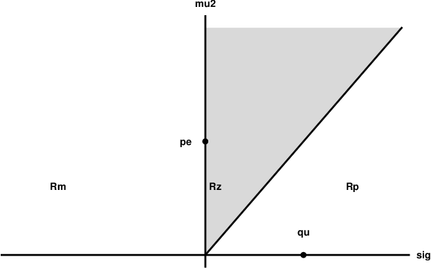
The same reasoning can be carried out to arbitrary odd dimension. First, define the regions
and also the limit regions
Consider representatives and (in canonical form) of points and in the regions and respectively. Then has a spacelike eigenplane with eigenvalue as well as timelike eigenvector and spacelike eigenplane with eigenvalue . Restricting to the subspace we can repeat the procedure followed for the five dimensional case and conclude that has simultaneously limits on the points and . Analogously has a spacelike eigenplane with eigenvalue as well as spacelike eigenvector and timelike eigenplane with eigenvalue . Restricting to the subspace , the above arguments for the five dimensional case show that has simultaneous limits on the points and . Thus the regions and limit simultaneously with and as and tend to zero respectively. Indeed, the same ideas can be applied again to and , so that they also limit simultaneously, as and go to zero respectively, with and . In general, the regions analogously defined, i.e. where gives the number of vanishing parameters and the subindex gives the sign of , have simultaneous limits in and , where the subindex 0 stands for vanishing .
For the even dimensional case (with ), notice that the canonical form (23) with is equivalent to the odd dimensional case direct sum with a one dimensional zero endomorphism (of a Riemannian line). Hence, the previous reasoning for odd dimensions also applies for even dimensions and . For example, consider in dimensions the regions and . Then they both assume limit in and . Notice that if we keep no degenerate limits of this kind occur. This can be justified as follows. Let be defined as in (14). Then, it can be readily checked that , so if , then . If we keep (thus both are different from zero), and make , the limit must have always . Hence, it is not possible that a limit ends at two points with different rank. Similarly, keeping , the limit always has and therefore, limits cannot be degenerate either. The generalization to arbitrary even dimensions with is also straightforward from the odd dimensional case discussed above, which we now summarize in the following remark:
Remark 5.2.
In the case of odd, consider the subset of given by
Define also the subsets of given by
Then in the quotient topology of the sequences of with limit at also have limit at .
In the case of even, first define as in (14) and let be the subspace of given by:
Define also the following subsets of
Then in the quotient topology of the sequences of with limit at also have limit at .
6 Conformal vector fields
One interesting applications of our previous results is based on the relation between skew-symmetric endomorphisms and the set of conformal Killing vector fields (CKVFs) of the -sphere, . These vector fields are the generators of the conformal transformations of the -sphere , i.e. the group of transformations that scale the spherical metric , , where is a smooth positive function of . A standard technique to describe these transformations consists in viewing as the (real) projectivization of the null future cone in , in such a way that is induced from the isometries of . This is discussed in detail for the four dimensional case in [26] and in arbitrary dimensions in [23] and in [28] (the latter considers arbitrary signature and the projectivization of the null ”cone” in , giving ). This procedure stablishes a group homomorphism , which is one-to-one when restricted to the orthochronous component .
The Euclidean space and are well-known to be conformally related via the stereographic projection , where denotes the point w.r.t. which the projection is taken. Observe that the stereographic projection depends not only on the point but also on the (signed) distance between and the plane onto which the projection is performed. We do not reflect this dependence in the notation for simplicity.
Hence, the composition of a transformation with the stereographic projection yields , which is a conformal transformation of . Strictly speaking, these transformations are not diffeomorphisms of , as they require to remove the two points satisfying and , which are the “preimage” and the “image” of infinity under respectively. Nevertheless, since is a group homomorphism, so is as well as the map which assigns . In that sense and are the same. These group homomorphisms, induce Lie algebra homomorphisms between , and (the vector fields generating ). The precise form of these maps depends, firstly, on the representative used to describe the projective cone (i.e. ) and secondly on the point as well as on the signed distance from this point to the plane. In [23], the morphism
| (44) |
is constructed33 3 The method in [23] is based on the unit spacelike hyperboloid in Minkowski instead of on the null cone. However, the two methods are easily seen to be equivalent to the one we describe related to each other using the representative with for the projective cone, where () are Minkowskian coordinates of , is the point with coordinates () and the image plane for the stereographic projection is . The result is a representation of where the vector vector fields are expressed in Cartesian coordinates induced from the Minkowskian coordinates by means of .
Theorem 6.1.
[[23]] Let endowed with Minkowskian coordinates and consider any element written in the basis in the form
| (45) |
where are column vectors, t stands for the transpose and is a skew-symmetric matrix (). Then, in the Cartesian coordinates of defined by the embedding , , the CKVFs of are
| (46) |
Moreover, for every and is a Lie algebra antihomomorphism, i.e. .
Remark 6.1.
For later use, we write explicitly the parameters of the vector field in terms of the entries of the endomorphism :
| (47) | ||||||
where capital Latin indices are lowered with the Kronnecker . Unless otherwise stated, without subindex refers to the map given in (44) while refers to the CKVF which is image under of the skew-symmetric endomorphism .
The freedom of choosing a representative for (as well as the point and the projection stereographic plane) can be also seen in a more “passive” picture. Consider two different sets of Minkowskian coordinates and related by a transformation , . Using Theorem 6.1, we obtain two different embeddings associated to and respectively, for which and , as well as two associated maps . Let , defined by (45) with parameters and in the bases and respectively. Then, can be associated to two vector fields
| (48) | ||||
| (49) |
which are equal in the following sense. If we transform the representative with , we obtain a new representative of the projective cone which in coordinates is precisely . Abusing the notation, the map is such that . Then, considering and as respresentations of the same space in two different global charts and , can be seen as a change of coordinates , with the property that the Euclidean metric in coordinates transforms as
| (50) |
for a smooth positive function . In other words, changing to different Minkowskian coordinates in induces a change of coordinates in in such a way that the form (46) of the map is preserved. Notice that a similar result holds if we change the point w.r.t. which we take the stereographic projection, because any two must be related by a transformation.
Therefore, for the rest of this section, we will often adapt our choice of Minkowskian coordinates of to simplify the problem at hand. With this choice, it comes a corresponding set of cartesian coordinates of such that is given by equation (46) and the Euclidean metric is . Which coordinates are adequate obviously depends on the problem. For example, from the block form (17) and (18) of skew-symmetric endomorphisms, consider each of the blocks as endomorphisms of , extended as the zero map in and respectively, and similarly for each . If we denote by and the corresponding images by , one readily gets following decomposition:
| (51) |
where in terms of , is given by
| (52) |
(because the dimension of the Minkowski space where is defined is , cf. Theorem 6.1). The explicit form of each of the terms in (51) is direct from (47). Namely, the terms and are given by (46) with vanishing parameters for and respectively, and each is proportional to a vector field of the form
| (53) |
with such that . More specifically, , where is given by equation (53) with and if even while if odd. Vector fields of the form (53) will play an important role in the following analysis. They have the form of axial Killing vector fields, although in general they are CKVFs because of the conformal factor in . From the previous discussion, it follows that there exists a conformal transformation such that . Then by the properties of the Lie derivative it is immediate
| (54) |
In other words, is an axial Killing vector of and is an axial Killing vector of . Thus, we define:
Definition 6.1.
A CKVF of an Euclidean metric , , is said to be a conformally axial Killing vector field (CAKVF) if and only if the exist a such that is an axial Killing vector field of . Equivalently, is a CAKVF if and only if it is an axial Killing vector field of .
Remark 6.2.
Using Theorem 6.1, it is immediate to verify that a CKVF is a CAKVF if and only if it is the image under of a simple unit spacelike endomorphism .
Notice that the terms in (51) form a commutative subset of . This is an immediate consequence of the fact that is a Lie algebra antihomomorphism (c.f. Theorem 6.1) and the blocks (resp. ) and are pairwise commuting. In addition, a straightforward calculation shows that they form an orthogonal set
| (55) |
where for even and for odd. In fact, as we show next, orthogonality of two CKVFs implies commutativity provided one of them is a CAKVF. If both are CAKVF, then orthogonality turns out to be equivalent to commutativity.
Lemma 6.2.
Let be non-proportional CAKVFs and a CKVF. Then if and only if there exist cartesian coordinates such that and . Equivalently if and only if . In addition, if .
Proof.
Let be such that . Since and are simple, spacelike and unit (cf. Remark 6.2), we can write and for spacelike, unit vectors , such that . By Corollary 4.2.1, it follows that if and only if are mutually orthogonal. Let us take cartesian coordinates of such that . Then, in the associated coordinates of it follows and . This proves the first part of the lemma. From this result, it is trivial that implies .
To prove that implies (which in particular establishes the converse for CAKVFs), let us take coordinates such that . Then, writing as a general CKVF (46), we obtain by direct calculation:
| (56) |
Therefore must vanish. This implies that the associated endomorphisms and to and adopt a block structure from which it easily follows that and hence . ∎
Definition 6.2.
Let . Then a decomposed form of is for an orthogonal subset , where are CAKVFs, for . A set of cartesian coordinates such that , for for odd and for even, is called a set of decomposed coordinates.
Remark 6.3.
Observe that the is a CKVF. By Lemma 6.2 and its proof, the parameters defining in a set of decomposed coordinates must all vanish except possibly when is even or when is odd. This means that there is a skew-symmetric endomorphism with restricts to ( even) or ( odd) and vanishes identically on their respective orthogonal complements such that . We will exploit this fact in an essential way below.
With the definition of decomposed form of CKVFs, we can reformulate Theorem 2.6 in terms of CKVFs.
Proposition 6.1.
Let . Then there exist an orthogonal set of CAKVFs such that . For every such a set and there exist such that . In addition,with the definition the expression provides a decomposed form of .
Proof.
The existence of commuting CAKVFs is a direct consequence of decompositions (17) and (18) of the associated skew-symmetric endomorphism , for even and odd respectively. Indeed, for each such decomposition of , it follows a set of CAKVFs commuting with . Let us denote any such set. Each is associated to a simple, spacelike unit endomorphism that commutes with . By Lemma 4.2, defines a spacelike eigenplane of . The orthogonality of any two such eigenplanes , is a consequence of Corollary 4.2.1 because . In other words, given a set of CAKVFs commuting with , we have a block form of , thus, defining , it is immediate that is a decomposed form with . ∎
The next step now is to give a definition of canonical form for CKVFs, which we induce from the canonical form of the associated skew-symmetric endomorphism.
Definition 6.3.
A CKVF is in canonical form if it is the image of a skew-symmetric endomorphism in canonical form, i.e. such that is given, in a cartesian set of coordinates denoted canonical coordinates, by the parameters if even and if odd (the non-specified parameters all vanish) and are CAKVFs , for for odd and for even, and where are given by Definition 3.2.
Given a CKVF , the existence of a canonical form and canonical coordinates are guaranteed by Theorem 3.3. By Theorem 6.1, the conformal class of a CKVF is equivalent to the equivalence class of under the adjoint action of , and this is determined by the canonical form of (c.f. Theorem 5.1). This argument together with the results of Section 5 yield the following statement.
Theorem 6.3.
Let be in canonical form. Then its conformal class is determined by if even and if odd. Moreover, the structure of corresponds with that of Remark 5.2.
Given a canonical form the set of vectors are pairwise commuting and linearly independent. As we will next prove, in the case of odd dimension this set is a maximal (linearly independent) pairwise commuting set of CKVFs commuting with (i.e. it is not contained in a larger set of linearly independent vectors commuting with ). In the case of even dimension it is not maximal. By Remark 6.3, , where the right-hand side denotes a CKVF of the form (53) whose parameters vanish, except possibly . As mentioned in the Remar, the corresponding skew-symmetric endomorphism satisfying can be understood as an element , with , that is identically zero in . Fix the orientation in so that the basis is positively oriented. The Hodge star maps two-forms into two-forms. This defines a natural map
| (57) |
From standard properties of two-forms, (see also [24]) it follows that commutes with . We may extend to an endomorphism on that vanishes identically on , just as . It is clear that the commutation property is preserved by this extension. The image of under is the vector field
| (58) |
which by construction commutes with . In the case that is the first element in a decomposed form , it is immediately true that also commutes with all of the CAKVFs . Hence, is a pairwise commuting set, all of them commuting with . This set can be proven to be maximal:
Proposition 6.2.
Let be a CKVF in canonical form. If is odd, is a maximal linearly independent pairwise commuting set of elements that commute with . If is even, is a maximal linearly independent pairwise commuting set of elements that commute with .
Proof.
Suppose that there is an additional CKVF commuting with each element in if odd or if even (in either case clearly commutes with also). Since it commutes with each , by Proposition 6.1, it admits a decomposed form , where is a CKVF orthogonal to each and which must verify . Equivalently, their associated endomorphisms satisfy , where denotes the centralizer of , i.e. the set of all skew-symmetric endomorphisms that commute with . From the results in [24], when is odd and when is even. Here, is the skew-symmetric endomorphim associated with and we restrict to because the action of the endomorphisms is identically zero in . Thus if odd and if even.
∎
7 Adapted coordinates
In the previous section we obtained a canonical form for each CKVF of euclidean space based on the canonical form of skew-symmetric endomorphisms in Section 3. As an application, we consider in this section the problem of adapting coordinates in to a given CKVF . The use of the canonical form will allow us to solve the problem for every possible essentially in one go. Actually it will suffice to consider the case of even dimension and assume that at least one of the parameters in the canonical form of is non-zero. The case where both and vanish will be obtained as a limit (and we will check that this limit does solve the required equations). The case of odd dimension wil be obtained from the even dimensional one by expliting the property that can be viewed as a hyperplane of in such a way that the given CKVF in extends conveniently to . Restricting the adapted coordinates already obtained in the even dimensional case to the appropriate hyperplane we will be able to infer the odd dimensional case. As we will justify the process of adapting coordinates is different for and even. The case has been treated in detail in [24], so it will suffice to consider even here.
Consider endowed with a CKVF . First of all we adapt the Cartesian coordinates of so that takes its canonical form and we fix the metric of to take the explictly flat form in these coordinates. We further assume (for the moment) that is even. For notational reasons it is convenient to rename the canonical coordinates44 4 The fact that we tag the coordinates with lower indices has no particular meaning. It is simply to avoid a notational clash of upper indices and powers that will appear later as and for , where in the even case case (see (52)). By Proposition 6.1, can be decomposed as a sum of CKVFs and and, additionally one can construct canonically yet another CKVF . This collection of CKVFs defines a maximal commutative set. Moreover, are all mutually orthogonal and perpendicular to and . It is therefore most natural to try and find coordinates adapted simultaneously to the whole family . This will lead a (collection of) coordinate systems where the components of are simply constants. From here one can immediately find coordinates that rectify , if necessary. It is important to emphasize that selecting the whole set to adapt coordinates provides enough restrictions so that the coordinate change(s) can be fully determined. Imposing the (much weaker) condition that the system of coordinates rectifies only is just a too poor condition to solve the problem. This is an interesting example where the structure of the canonical decomposition of (or of ) is exploited in full.
By Theorem 6.1, the explicit form of in the canonical coordinates is
| (59) | ||||
| (60) | ||||
| (61) |
We are seeking coordinates adapted to these vector fields, i.e. such that . It is clear that if is an adapted coordinate system, so it is for arbitrary functions , and , where . This will be used to simplify the process of integration. This freedom, may be restored at the end if so desired. Hence
| (62) | ||||||||||
| (63) | ||||||||||
| (64) |
The additional coordinates , will appear through functions of integration. It is clear that the structure of the equations is different for , where there are no , which implies that the process of integration follows a different route. The case has been treated in full detail in [24], where the the complex structure of can be exploited to simplify the problem. Here we adress the problem for which we assume from now on.
We may start by integrating (64). The first pair gives , so that the second pair becomes a harmonic oscillator in , whose solution is
| (65) |
where and are arbitrary functions (depending only on the variables indicated) and is not identically zero.
Inserting (65) in any of the two right-most equations of (62) and (63) and equating terms multiplying and yields:
Thus, is a function only of , which may be absorbed on the coordinate as discussed above. The two first equations imply
for arbitrary (non-zero) functions and . Defining we can write
where , with , form a set of arbitrary (non-zero) functions of such that . The function satisfies
| (66) |
Inserting (66) in the two left-most equations in (62) and (63), with the change of variable , we obtain after some algebra the following covariant system of PDEs (indices refer to )
| (67) |
and where is the Levi-Civita covariant derivative of .
Lemma 7.1.
Up to shifts and , the general solution of (67) with either or non-zero is given by
| (68) |
where is a function of integration (depending on ), and , , with given by (14). The solution (68) admits a limit (i.e. ) provided , which is
| (69) |
Up to shifts and , this function is the general solution of (67) for .
Proof.
The coordinates defined in the lemma diagonalize and simultaneously and yield
| (70) |
From this and equation (67) it follows that or, equivalently, . Substracting the and components of (67) one obtains
| (71) |
for an arbitrary separation function . The general solution is clearly
| (72) |
where are also functions of . Since drops out in we may set w.l.o.g. Inserting (72) in (any of) the diagonal terms of (67) and one simply gets
| (73) |
Hence and we may use the freedom of translating by a function of to write (i.e. ). A similar translation in sets . Rescaling the functions as and we get
| (74) |
It is obvious that . Thus taking as the positive root and adding a multiplicative sign in (74), we obtain (68). To evaluate the convergence as both tend to zero, or equivalently , consider the series expansion
where denotes a sum of homogeneous polynomials in starting at order four, whose coeficients may depend on and . Then, the expansion of is
| (75) |
It is clear that and the rest of the equation converges if and only if in which case the limit is (69). An easy calculation shows that this limit is (up to shifts in ) is the general solution of (67) when . ∎
Having the general general solution (68) of (67) we can give the expression of the adapted coordinates
| (76) | ||||
| (77) | ||||
| (78) |
where no sign of is in principle assumed55 5 The domain of definition of will be later restricted under the condition that the adapted coordinates define a one to one map., except for the case , where must be understood as the limit (with ) (69) and , . This coincides with the limit of the RHS expressions (76), (77), which is
| (79) |
From equations (76), (77) and (78) it is obvious that the sign is not relevant in the definition of the adapted coordinates. This is because the two branches and correspond with and respectively, which in terms of the adapted coordinates, is equivalent to a rotation of in the angles. Hence, w.l.o.g. we consider , i.e. . Also notice that the dependence on the variables appears through the functions and , with . The set define independent arbitrary functions of the variables , so it is natural to use as coordinates themselves, provided they are restricted to satisfy .
We now calculate the region of covered by the adapted coordinates. It is clear that in no case this region can include neither the zeros of the vector fields and and nor the points where these vectors are linearly dependent. We therefore start by locating those points. Denoting the loci of the zeros of and and by , and respectively, a simple calculation gives
| (80) | ||||
| (81) | ||||
These expressions are valid for every value of and imply that in the case , , which is contained in each .
On the other hand, since is an orthogonal set of CKVFs (cf. Lemma 6.2), they are pointwise linearly independent at all points where they do not vanish. Similarly, is also an orthogonal set, so linear independence is guaranteed away from the zero set. Away from this set, the set of vectors is linearly dependent only at points where and are proportional to each other with a non-zero proportionality factor, , . One easily checks that, away from and , the set of point where vanishes is empty except when and . It turns out to be useful to determine the set of points where when at least one of is non-zero. We call this set , and a straightforward analysis gives
Obviously, the two expressions are equivalent when both and are non-zero. The interest of this set is that it happens to always contain and . This, together with the fact that when these sets are contained in the axes will allow us to ignore them altogether.
Lemma 7.2.
Assume that at least one of is non-zero. Then .
Proof.
Let us define the following auxiliary coordinates
| (84) |
Except for the case (which will be analyzed later) the coordinates obviously cover . In terms of the adapted coordinates, they read
| (85) |
Let us analyze the points where (85) fails to be a change of coordinates and hence restrict the domain of definition of . The first thing to notice is that a change of sign in the coordinate is equivalent to a rotation of angle in the coordinate . Moreover, at points where , i.e. the axis of , the coordinate is completely degenerate, which obviously excludes from the region covered by the adapted coordinates. To avoid duplications, we must restrict and or alternatively and . We choose the former for definiteness.
The hypersurface is an dimensional sphere of radius , namely . This gives a straightforward splitting of , with , into , where is foliated by dimensional spheres. The set respects this foliation, so it descends to (the last factor is the radius of the sphere). To avoid extra notation we also use to denote this quotient set. We next show that the adapted coordinates actually cover the largest possible domain, namely . From the previous discussion, this is a consequence of the following result.
Lemma 7.3.
Assume that at least one of is not zero. Then. the transformation
| (86) |
is a diffeomorphism.
Proof.
The determinant of the jacobian of (86) reads
| (87) |
Since is strictly positive (cf. (68) and recall that we chose w.l.o.g.), the conflictive points are . To calculate the locus we obtain the inverse transformation of in terms of by solving (68) and the first two in (85). The result is, after a straightforward computation,
| (88) |
It follows that is equivalent to and . When translated into the original coordinates this set is precisely . Also, from (88) it is obvious that is multivalued, which also implies that is multivalued after substituting as a function of in the first equation in (85)66 6 This was already evident by observing that a change of sing in is cancelled by a rotation of in . We solve this issue by restricting to be strictly positive and let take values in . ∎
We have shown that the adapted coordinates cover all except . The domain of definition of the coordinates depends on and , because . This defines a band , whose width and tilt is determined by through (see figure 2). Nevertheless, the coordinate change is well defined for all values of and and involves only periodic functions of . Thus, we can extend the domain of definition of to all of . This defines a covering of the original space which unwraps completely the orbits of and . It is not the universal covering because it does not unwrap the orbits of the axial vectors. This result is a generalization to higher dimensions of the covering dicussed in detail in [24].
The limit case (that is ) corresponds with a band of infinite width, i.e. . In this case, the adapted coordinates also cover the largest possible set . Recall that in this case the only points where is not a linearly independent set is the union of , and and we have already seen that in this case , for . This limit case is the same result that we would have obtained, had we performed a direct analysis using as given by (69).

Once we have determined the adapted coordinates and the region they cover, we may proceed to calculate the expression of the Euclidean metric
| (89) |
in adapted coordinates. We start with the term , which is straightforward
| (90) |
where in the last equality we used , which follows from and we have defined
| (91) |
The notation is justified because the right-hand side corresponds to the standard unit metric on . This follows because is obviously flat and the restriction defines a unit sphere. We emphasize, however that the notation refers to the quadratic form above, not to the spherical metric in any other coordinate system. Observe also that in (90) should be understood as a short name for the explicit differential of in terms of , . Using (89) and (90), we have
| (92) |
which after a explicit calculation reduces to
| (93) |
Notice that , and . From the expressions in cartesian coordinates it is straightforward to show
| (94) |
where we have used (see (78)). Thus
| (95) |
The remaining terms are rather long to calculate. With the aid of a computer algebra system one gets
| (96) | ||||
| (97) | ||||
| (98) |
Notice that no terms in appear but those in , since neither nor depend on . Putting all these results together we obtain the following expression:
Lemma 7.4.
In adapted coordinates , the Euclidean metric takes the form
| (99) |
We would like to stress the simplicity of this result. Except in the a global conformal factor, the metric does not depend in and (so, both and are Killing vectors of ). The dependence in the coordinate and the conformal class constants is also extremely simple. Even more, the fact that all dependence in arises only in allows us to use any other coordinate system on the unit . Any such coordinate system is still adapted to and but (in general) no longer to . This enlargement to partially adapted coordinates is an interesting consequence of the foliation of by -spheres described above.
We now work out the odd case. As already discussed, we will base the analysis on the even dimensional case by restricting to a suitable a hyperplane. The underlying reason why this is possible is given in the following lemma.
Lemma 7.5.
Fix odd. Let be a CKVF of in canonical form and let be canonical coordinates. Consider the embedding where is identified with the hyperplane , for a cartesian coordinate of . Then extends to a CKVF of with the same value of and .
Proof.
By Remark 6.3 and Theorem 6.1, the expression of in the canonical coordinates is
Define on in cartesian coordinates by where is given by (59) with . It is clear that this vector is a CKVF of written in canonical form, that it is tangent to the hyperplane and that it agrees with on this submanifold. ∎
Consequently, introducing adapted coordinates for the extended CKVF and restricting to will provide adapted coordinates for . The restriction will obviously reduce the domain of definition of the adapted coordinates to a hypersurface. It is straightforward from equation (77) and the second equation in (79) that for the three cases , or , the hyperplane corresponds to . It follows that the remaining coordinates are adapted to and all . Their domain of definition is , , , and the coordinate change is given by (76) (or the first in (79)) together with (78) after setting and . Depending on the sign of one gets for
| (100) |
where
| (101) |
and for all three cases
| (102) |
where we write for the function or according with sign of .
The range of variation of was inferred before from the corresponding range of variation of in . It may happen, however, that when we restrict to the hyperplane , the range gets enlarged and additional points get covered by the adapted coordinate system. The underlying reason is that, in effect, we are no longer adapting coordinates to , so the points on where this vector is linearly dependent to (or zero) are no longer problematic. When , one has
We may ignore the case because . It follows from (80) and (7) that
When , the two sets are the same and no extension of the coordinates is possible. However, when , the set is strictly larger than . From expressions (100) and (102) one checks that corresponds exactly to the value and that is at the limit . Thus, a priori there is the possibility that the adapted coordinates can be extended regularly to when . It follows directly from (100) that this is indeed the case (observe that, to the contrary, the limit in (100) is singular when , in agreement with the previous discussion). Thus, the range of definition of is when . The conclusion is that, irrespectively of the value of , the adapted coordinates cover the largest possible domain of , namely all points where is non-zero away from the axes of .
To obtain the Euclidean metric in for odd in adapted coordiantes we simply restrict (99) (with ) to the hypersurface , and get
| (103) |
where respectively if .
Remark 7.1.
The three odd dimensional cases can be unified into one. The function coincides with the limits of and when . However, the analytical continuation of to negative values of does not directly yield . To solve this we introduce the function
which is analytic in and takes real values for real . We observe that for , () and (). This suggests introducing the coordinate change for and for . From the domain of , it follows that takes values in when and when . In terms of , the three metrics metric take the unified form
The function is the analytic continuation of to negative values of . We could have started with and continued analytically to positive values of . Instead of repeating the argument, we simply introduce a new variable defined by with range of variation for and for . The metric takes the (also unified and even more symmetric) form
The function is again analytic in , takes real values on the real line, and now it extends . More specifically, (), () and ().
Remark 7.1 allows us to work with all the odd dimensional cases at once, which will be useful for Section 8. However, this unified form does not arise naturally when the odd dimensional case is viewed as a consequence of the even dimensional case. So, leaving aside this remark for Section 8, we summarize the results of this section in the following Theorem.
Theorem 7.6.
Given a CKVF of , with even, in canonical form , the coordinates , for and , defined by
| (104) |
with
| (105) |
which admits a limit , furnish adapted coordinates to , which cover the maximal possible domain, namely for , , and . Moreover, the metric , which is flat in canonical cartesian coordinates, is given by
| (106) |
If is odd and is in canonical form, , the coordinates adapted to are given by the case of (even) dimensions, for restricted to (which defines the embedding ) and cover again the maximal possible domain, given by for , , and when and when . Moreover, the metric , which is flat in canonical cartesian coordinates, is given by the pull-back of (106) at after setting . Explicitly is, depending on the sign of , given by (103) with as in (91).
8 TT-Tensors
The adapted coordinates derived in Section 7 provide a useful tool to solve geometric equations involving CKVFs. In this section we give an example of this in the context of -vacuum spacetimes admitting a smooth null conformal infinity.
Recall that for such spacetimes the data at is a conformal class of riemannian metrics and a conformal class of transverse and divergence-free tensors. More specifically, for a representative metric in the conformal class, there is associated a symmetric tensor satisfying (divergence-free) and (transverse). For any other metric in the conformal class, the associated tensor is , which is again a TT tensor with respect to . In dimension , it has been shown in [25] that the spacetime generated by the Cauchy data at admits a Killing vector if and only if the metric admits a CKV (which is the restriction of the Killing vector to ) and satisfies the so-called Killing initial data (KID) equation. This equation admits a natural generalization to arbitrary dimension which is
| (107) |
where is the divergence of . Equation (107) reduces to the KID equation of Paetz in dimension and it is conformally covariant, i.e. if is a solution, then so it is . We emphasize however, that in higher dimension () it is not known whether a spacetime admiting a smooth such that the corresponding data at null infinity solves the KID equation for some CKV , must necessarily admit a Killing vector.
A CKVF satisfying (107) will be called KID vector for short. An important property of KID vectors is that they form a Lie subalgebra of CKVFs, i.e. if are KIDs for a given tensor , then is also a KID for . The problem of obtaining all TT-tensors with generality for a given conformal structure is hard, even in the conformally flat case (see e.g. [3]). In this section we exploit the results above to obtain the general solution of the KID equations in dimension for spacetimes which possess two commuting symmetries, one of which is axial. This case is specially relevant since corresponds to the physical case of four spacetime dimensions and the class necessarily contains the Kerr-de Sitter family of spacetimes, which is a particularly interesting explicit familiy of spacetimes. Our strategy is to take an arbitrary CKVF , derive its canonical form , adapt coordinates to and and impose the KID equations to and . The problem simplifies notably in the conformal gauge to because both and become Killing vector fields. From Remark 7.1, we may treat all cases at the same time by using the form of the metric
| (108) |
We remark that even though we solve the problem by fixing the coordinates and conformal gauge, we shall write the final result in fully covariant form (cf. Theorem 8.2 below).
In the conformal gauge of , the condition that a TT-tensor satisfies KID equations for both and (which is equivalent to imposing that and are KID vectors) is trivial in the adapted coordinates obtained in the previous section:
| (109) |
Thus, are only functions of . The transversality condition is also quite simple in adapted coordinates:
| (110) | ||||
| (111) | ||||
| (112) |
while the traceless condition imposes
| (113) |
There are no equations for so with an arbitrary function. The general solution of equations (111) and (112) is obtained at once and reads
| (114) |
For equations (110) and (113), we let be an arbitrary function and obtain the remaining components
| (115) |
Summarizing
Lemma 8.1.
In the three-dimensional conformally flat class , let be a CKVF. Decompose in canonical form and fix the conformal gauge so that given by (108). Then the most general symmetric TT-tensor satifying the KID equations for and simultaneously is, in adapted coordinates , a combination (with constants) of the following tensors
| (116) | ||||
| (117) |
where and are arbitrary functions of .
Having obtained the general solution in a particular gauge, our next aim is to give a (diffeomorphism and conformal) covariant form of the generators in Lemma 8.1. From [23], we know that, for any CKV of any -dimensional metric (not necessarily conformally flat) the following tensors are TT w.r.t. to and satisfy the KID equation with respect to .
| (118) |
where denotes the norm w.r.t. and the contravariant form of . Thus, we can rewrite as
| (119) |
We now restore the conformal gauge freedom by considering the metric and , for any (positive) conformal factor . Since the tensors are already conformal and diffeomorphism covariant, we must impose their multiplicative factors in to be conformal and diffeomorphism invariant. With the gauge freedom restored, the norms of the CKVFs now are
| (120) |
Then, considering as function of the conformal invariant quantity , one can directly cast in the following form:
| (121) |
which is a conformal and diffeomorphism covariant expression. Notice that the expression is symmetric under the interchange because the coefficient of expressed in the variable is identical in form to the coefficient of .
For the tensor , redifining , it is immediate to write
| (122) |
which is obviously conformal and diffemorphism covariant if and only if is conformal invariant, e.g. considering . We remark that the form (122) already appeared (with different powers due to the different dimension) in the classification [24] of TT tensors in dimension two satisfying the KID equation.
For the remaining tensors and , we define a conformal class of vector fields , which in the original gauge coincides with . This vector is divergence-free , and this equation is conformally invariant provided the conformal weight of is (i.e. for , the corresponding vector is ). We therefore impose this conformal behaviour of .77 7 This choice may appear somewhat ad hoc at this point. However, the condition of vanishing divergence appears naturaly when studying (for more general metrics) under which conditions a tensor is a TT tensor satisfying the KID equation for . We leave this general analysis for a future work. The direction of is fixed by orthogonality to and . The combination of norms that has this conformal weight and recovers the appropriate expression in the gauge of Lemma 8.1 is (note that the orthogonality and norm conditions fix uniquely up to an irrelevant sign in any gauge). Thus, we may write
| (123) |
which are conformally covariant expressions. Therefore, we get to the final result:
Theorem 8.2.
Let be a CKVF of the class of three dimensional conformally flat metrics and let a canonical form. For each conformal gauge, let us define a vector field with norm , orthogonal to and . Then, any TT-tensor satisfying the KID equations (107) for and is a combination (with constants) of the following tensors:
| (124) | ||||||
| (125) |
for arbitrary functions and of .
Remark 8.1.
The vector field defined in this Theorem is divergence-free. This property would have been difficult to guess (and even to prove) in the original Cartesian coordinate system.
Remark 8.2.
A corollary of this theorem is that the general solution of the -vacuum Einstein field equation in four dimensions with a smooth conformally flat null infinity and admitting an axial symmetric and a second commuting Killing vecor can be parametrized by two functions of one variable and two constants. Recall that in the case, the general asympotically flat stationary and axially symmetric solution of the Einstein field equations can be parametrized (in a neighbourhood of spacelike infinity, by two numerable sets of mass and angular multipole moments (satisfying appropriate convergence properties), see [1], [4], [6] for details. There is an intriguing paralelism between the two situations, at least at the level of crude counting of degrees of freedom. This suggests that maybe in the case it is possible to define a set of multipole-type moments that characterizes de data at null infinity (and hence the spacetime), at least in the case of a conformally flat null infinity. This is an interesting problem, but well beyond the scope of the present paper.
Remark 8.3.
It is natural to ask whether Theorem 8.2 is general for TT-tensors admitting two commuting KIDs, , without the condition of being conformally axial. In Appendix of [23] one can explicitly find, for an arbitrary CKVF , the set of elements that commute with . Then, from a case by case analysis, one concludes that except in one special situation, for any linearly independent pair , with it is the case that there is a CAKVF such that . Thus, all these cases are covered by Theorem 8.2. The exceptional case is when are conformal to translations. It is immediate to solve the TT and KID equations for such a case directly in Cartesian coordinates.
The solution given in Theorem 8.2 provides a large class of initial data, which we know must contain the so-called Kerr-de Sitter-like class with conformally flat (see [23] for precise definition and properties of this class), which in turn contains the Kerr-de Sitter family of spacetimes. It is interesting to identify this class within the general solution given in Theorem 8.2. The characterizing property of the Kerr-de Sitter-like class in the conformally flat case is for some CKVF , where moreover, only the conformal class of matters to determine the family associated to the data. Decomposing canonically , a straightforward computation yields
| (126) |
which comparing with Theorem 8.2 yields the following corollary:
Corollary 8.2.1.
The Kerr-de Sitter-like class with conformally flat is determined by the TT-tensor with
| (127) |
It is also of interest to identify the the Kerr-de Sitter family. To that aim we combine the results in [23] to those in the present paper to show that this family corresponds to . The classification of conformal classes of in [23] is done in terms of the invariants and together with the rank parameter , where and are the coefficients of the characteristic polynomial of the skew-symmetric endomorphism associated to . In terms of these objects, it is shown in [23] that the Kerr-de Sitter family corresponds to either and , or and , the latter defining the Schwarzschild-de Sitter family. It is immediate to verify that, since (cf. Corollary 3.3.1) and , then and (the condition implies and implies ). Thus, in terms of the classification developed in this paper, the Kerr-de Sitter family corresponds to . It is interesting that in the present scheme we no longer need to specify the rank parameter to identify the Kerr-de Sitter family (unlike in [23]) and that the whole family is represented by an open domain. We emphazise that the dependence in in the solutions given in Theorem 8.2 and Corollary 8.2.1 is implicit through the norm of .
Acknowledgements
The authors acknowledge financial support under the projects PGC2018-096038-B-I00 (Spanish Ministerio de Ciencia, Innovación y Universidades and FEDER) and SA083P17 (JCyL). C. Peón-Nieto also acknowledges the Ph.D. grant BES-2016-078094 (Spanish Ministerio de Ciencia, Innovación y Universidades).
References
- [1] A. E. Aceña. Convergent null data expansions at space-like infinity of stationary vacuum solutions. Annales Henri Poincaré, 10, 275–337, 2009.
- [2] M. T. Anderson. Existence and stability of even-dimensional asymptotically de Sitter spaces. Annales Henri Poincaré, 6, 801–820, 2005.
- [3] R. Beig. TT-tensors and conformally flat structures on 3-manifolds. Banach Center Publications, 41, 109–118, 1997.
- [4] R. Beig and B. G. Schmidt. Time independent gravitational fields. Lect. Notes Phys., 540, 325–372, 2000.
- [5] N. Burgoyne and R. Cushman. Conjugacy classes in linear groups. Journal of Algebra, 44, 339 – 362, 1977.
- [6] T. Bäckdahl. Axisymmetric stationary solutions with arbitrary multipole moments. Classical and Quantum Gravity, 24, 2205–2215, 2007.
- [7] Y. Choquet-Bruhat. General Relativity and the Einstein Equations. Oxford Mathematical Monographs. OUP Oxford, 2008.
- [8] R. Cushman and W. van der Kallen. Adjoint and coadjoint orbits of the poincaré group. Acta Applicandae Mathematicae, 90, 65–89, 2006.
- [9] D. Z. Djoković, J. Patera, P. Winternitz, and H. Zassenhaus. Normal forms of elements of classical real and complex lie and jordan algebras. Journal of Mathematical Physics, 24, 1363–1374, 1983.
- [10] F. Fernández-Álvarez and J. M. M. Senovilla. Gravitational radiation condition at infinity with a positive cosmological constant. Phys. Rev. D, 102, 101502, 2020.
- [11] Y. Fourès-Bruhat. Théorème d’existence pour certains systèmes d’équations aux dérivées partielles non linéaires. Acta Math., 88, 141–225, 1952.
- [12] H. Friedrich. Existence and structure of past asymptotically simple solutions of Einstein’s field equations with positive cosmological constant. Journal of Geometry and Physics, 3, 101 – 117, 1986.
- [13] H. Friedrich. Conformal Einstein Evolution. Springer Berlin Heidelberg, Berlin, Heidelberg, 2002.
- [14] H. Friedrich and A. Rendall. The cauchy problem for the einstein equations. In Bernd G. Schmidt, editor, Einstein’s Field Equations and Their Physical Implications, Berlin, Heidelberg, 2000. Springer Berlin Heidelberg.
- [15] F.R. Gantmacher. The theory of matrices. Vol. 1 The Theory of Matrices. Chelsea Pub. Co., 1960.
- [16] R. Goodman and N.R. Wallach. Symmetry, Representations, and Invariants. Graduate Texts in Mathematics. Springer New York, 2009.
- [17] B.C. Hall. Lie Groups, Lie Algebras, and Representations: An Elementary Introduction. Graduate Texts in Mathematics. Springer, 2003.
- [18] G. S. Hall. Symmetries And Curvature Structure In General Relativity. World Scientific Lecture Notes In Physics. World Scientific Publishing Company, 2004.
- [19] D. Ida. Complete integrability of cohomogeneity-one strings in and canonical form of Killing vector algebra. Journal of Mathematical Physics, 61, 082501, 2020.
- [20] A.W. Knapp. Lie Groups Beyond an Introduction. Progress in Mathematics. Birkhäuser Boston, 2002.
- [21] K. Lange. Optimization. Springer Texts in Statistics. Springer New York, 2013.
- [22] A. Lichnerowicz. Théories relativistes de la gravitation et de l’électromagnétisme: relativité générale et théories unitaires. Collection d’ouvrages de mathématiques à l’usage des physiciens. Masson, 1955.
- [23] M. Mars, T-T Paetz, and J. M. M. Senovilla. Classification of Kerr–de Sitter-like spacetimes with conformally flat . Classical and Quantum Gravity, 34, 095010, 2017.
- [24] M. Mars and C. Peón-Nieto. Skew-symmetric endomorphisms in : A unified canonical form with applications to conformal geometry. Classical and Quantum Gravity, 2020. DOI: 10.1088/1361-6382/abc18a
- [25] T-T Paetz. Killing Initial Data on spacelike conformal boundaries. Journal of Geometry and Physics, 106, 51 – 69, 2016.
- [26] R. Penrose and W. Rindler. Spinors and Space-Time: Volume 1, Two-Spinor Calculus and Relativistic Fields. Cambridge Monographs on Mathematical Physics. Cambridge University Press, 1984.
- [27] G. Y. Rainich. Electrodynamics in the general relativity theory. Proceedings of the National Academy of Sciences, 10, 124–127, 1924.
- [28] M. Schottenloher. A Mathematical Introduction to Conformal Field Theory. Lecture Notes in Physics. Springer Berlin Heidelberg, 2008.
- [29] J.L. Synge. Relativity: The Special Theory. Series in physics. North-Holland Publishing Company, 1956.
- [30] L. B. Szabados and P. Tod. A review of total energy–momenta in gr with a positive cosmological constant. International Journal of Modern Physics D, 28, 1930003, 2019.