On the identification of piecewise constant coefficients in optical diffusion tomography by level set

J. P. Agnelli Thanks: FaMAF-CIEM, Universidad Nacional de Córdoba, Medina Allende s/n 5000, Córdoba, Argentina. (agnelli@famaf.unc.edu.ar). A. De Cezaro Thanks: Institute of Mathematics Statistics and Physics, Federal University of Rio Grande, Av. Italia km 8, 96201-900 Rio Grande, Brazil (decezaromtm@gmail.com). A. Leitão Thanks: Department of Mathematics, Federal University of St. Catarina, P.O. Box 476, 88040-900 Florianópolis, Brazil (aleitao@mtm.ufsc.br). M. Marques Alves Thanks: Department of Mathematics, Federal University of St. Catarina, 88040-900 Florianópolis, Brazil (maicon.alves@ufsc.br).

August 11, 2026

Abstract

In this paper, we propose a level set regularization approach combined with a split strategy for the simultaneous identification of piecewise constant diffusion and absorption coefficients from a finite set of optical tomography data (Neumann-to-Dirichlet data). This problem is a high nonlinear inverse problem combining together the exponential and mildly ill-posedness of diffusion and absorption coefficients, respectively. We prove that the parameter-to-measurement map satisfies sufficient conditions (continuity in the $L^{1}$ topology) to guarantee regularization properties of the proposed level set approach. On the other hand, numerical tests considering different configurations bring new ideas on how to propose a convergent split strategy for the simultaneous identification of the coefficients. The behavior and performance of the proposed numerical strategy is illustrated with some numerical examples.

2000 Mathematics Subject Classification: 49N45, 65N21, 74J25.

Key words: Optical Tomography, Parameter Identification, Level Set Regularization, Numerical Strategy .

1 Introduction

Optical tomography has demonstrated to be a powerful technique to obtain relevant physiological information of tissues in a non-invasive manner. The technique relies on the object under study being at least partially light-transmitting or translucent, so it works best on soft tissues such as breast and brain tissue [24, 19]. By monitoring spatial-temporal variations in the light absorption and scattering properties of tissue, regional variations in hemoglobin concentration or blood oxygen saturation can be calculated. For a complete overview on optical tomography modalities the reader can consult the topical reviews [1, 17] and references therein.

A full description of light propagation in tissue is provided by the radiative transport equation. However, in this contribution we are interested in the so called static diffuse optical tomography (DOT). In DOT, light in the near infrared spectral region is used to measure the optical properties of physiological tissue. In this case, denoting the photon density by $u$ , the equation to consider is the following:

	$\displaystyle-\nabla\cdot(a(x)\nabla u)+c(x)u$	$\displaystyle=0\quad\mbox{in}\,\,\Omega$		(1)
	$\displaystyle a(x)\frac{\partial u}{\partial\nu}$	$\displaystyle=g\quad\mbox{on}\,\,\Gamma\,,$		(2)

where $\Omega\subset\mathbb{R}^{N}$ , $N\in\{2,3,4\}$ , is open, bounded and connected with Lipschitz boundary denoted by $\Gamma$ , the diffusion and absorption coefficients $a(x)$ and $c(x)$ , respectively, are measurable real-valued functions and $\nu$ is the outer-pointing normal vector. Moreover, $g\in H^{-1/2}(\Gamma)$ is the Neumann boundary data. Such boundary condition can be interpreted as the exitance on $\Gamma$ .

It is worth mentioning that equation (2) is a simplified way of modeling light fluence boundary condition in diffuse optical tomography, since a more realistic description is to consider a Robin boundary condition [28, 27]. However, we believe that our simplified boundary model already contains the essential aspects for the theoretical study that we present in this work. Further, this setting agrees with the uniqueness identification result derived by Harrach in [18]. For more details about boundary conditions in light propagation models we recommend to consult [28, 27] and references therein.

Since the optical properties within tissue are determined by the values of the diffusion and absorption coefficients, the problem of interest in DOT is the simultaneous identification of both coefficients from measurements of near-infrared diffusive light along the tissue boundary.

In this contribution, we proposed a level set regularization approach [15, 10, 7, 8] combined with a split strategy for the simultaneous identification of piecewise constant diffusion $a(x)$ and absorption $c(x)$ coefficients in (1)–(2), from a finite set of available measurements of the photon density $h:=u|_{\Gamma}$ , corresponding to inputs $g\in H^{-1/2}(\Gamma)$ in (1)–(2).

Related works: In [22], a Levenberg–Marquardt method for recovering internal boundaries of piecewise constant coefficients of an elliptic PDE as (1) was implemented. The proposed method is based on the series expansion approximation of the smooth boundaries and on the finite element method. However, in [22], there is not a theoretical result that guarantees regularizing properties of the iterated approximated solution. Indeed, as far as the authors are aware, there is not theoretical regularization approaches in the literature for recovering the pair of coefficients $(a,c)$ in (1) from boundary data.

In [31], the authors did a carefully designed experiment aimed to provide solid evidence that both absorption and scattering images of a heterogeneous scattering media can be reconstructed independently from diffuse optical tomography data. The authors also discuss the absorption scattering cross-talk issue.

Although it is well known that the identification of $a$ and $c$ simultaneously is not possible in a general case [2], recently B. Harrach [18] obtained a uniqueness result for the simultaneous recovery of $a$ and $c$ in (1)–(2) assuming that $a\geq a_{0}>0$ is piecewise constant and $c\in L^{\infty}_{+}$ ²² 2 The subscript ${}^{\prime}+^{\prime}$ denotes positive essential infima. is piecewise analytic. Under this condition both parameters are simultaneously uniquely determined by knowledge of all possible pairs of Neumann and Dirichlet boundary values $a\partial_{\nu}u|_{\tilde{\Gamma}}$ and $u|_{\tilde{\Gamma}}$ on an arbitrarily small open set $\tilde{\Gamma}$ of the boundary $\Gamma$ . The difference between the work of B. Harrach [18] and our work is that here we are considering a more practical approach: we only have access to a finite number of Neumann-Dirichlet pairs.

We also remark that the quantitative photoacoustic tomography problem (QPAT), in the diffusive approach, also aims to simultaneous recover $(a,c)$ of an elliptic boundary valued problem. See for example [29] and references therein. However, in the QPAT situation the solution of the “first inverse problem” generate internal data for the reconstruction. In this sense, the QPAT problem is very different to the identification problem that we are facing here.

Novelties: The novelties of this contribution are divided as follow:

•

We prove the continuity of the parameter-to-measurement (forward) map $F$ (defined in (3)) in the $[L^{1}(\Omega)]^{2}$ topology. It is done in Theorem 3 of Section 2, and it is possible thanks to a generalization of Meyers’ Theorem [23] that prove the regularity of the solution of (1)–(2) in $W^{1,p}(\Omega)$ for some $p>2$ (see Theorem 1). The proof of Theorem 1 is presented in detail in the Appendix.

In Section 3, we introduce a level set approach. In contrast to the seminal approach of Santosa on level set for inverse problems [26], our approach consists in a parametrization of the non-smooth admissible set of parameters with a pair of $H^{1}(\Omega)$ functions concatenated with a restriction of the search space using nonlinear constraints. Such approach allows us to enforce the desired additional properties on the pair of parameters $(a,c)$ (namely: $(a,c)$ is a pair of piecewise constant functions describing the high diffusion and absorption contrast between the optical properties of the object) that are not smooth.

Given the continuity of $F$ in the $[L^{1}(\Omega)]^{2}$ topology, it is now a standard result to prove that the level set approach is a regularization method as in the classical theory of regularization [7, 8, 10, 11]. Therefore, we only point out the convergence and stability results without a formal proof in Subsection 3.2.
•

Another contribution of the proposed level set approach is related to the numerical implementation presented in Section 5. It is worth to remind the reader that we aim to simultaneous reconstruct the pair $(a,c)$ of piecewise constant functions from a finite set of optical measurements. With this aim, we first run several numerical experiments in order to recover the absorption coefficient $c$ , based on either total or partial knowledge of $a$ . From this experiments we observed that the level set method for identifying $c$ performs well, even if a good approximation of the exact value of $a$ is not known. This is presented in Subsection 5.1. After that, in Subsection 5.2 we run another set of experiments but now concerning the identification of the diffusion coefficient $a$ , based on either total or partial knowledge of $c$ . In this case, we observed that the level set method for identifying $a$ performs well if a good approximation of the exact value of $c$ is available, but may generate a sequence $a_{k}$ that does not approximate the exact $a$ if the initial guess for the coefficient $c$ is far from its exact value. Such features of the identification problems suggested one of the main results related to the numerical perspective presented in Subsection 5.3. Given a initial guess $(a_{0},c_{0})$ , we adopted the strategy to “freeze” the coefficient $a_{k}=a_{0}$ during the first iterations, and to iterate the algorithm only with respect to the coefficient $c$ . We follow this strategy until the iterated sequence $c_{k}$ stagnates. Then, we freeze the absorption coefficient $c=c_{k}$ and iterate the algorithm only with respect to $a$ until the iterated sequence $a_{k}$ stagnates. Finally, we iterate both coefficients simultaneously. This numerical strategy has not only demonstrated that gives very good results but also reduces significantly the computational effort.

This article is organized as follows. In Section 2 we first introduce the parameter-to-measurement (forward) map F and after that, in Theorem 3, the continuity of this forward map is demonstrated. Then, in Section 3 we present the level set approach, we introduce the concept of generalized minimizers for an appropriate energy functional and we establish the regularization properties. In other words, we prove the well-posedness result and also convergence results for exact and noisy data. In Section 4, we introduce a smooth functional that is used in the numerical examples. We prove that the minimizers of such functional converge to a minimizer of the early energy functional in appropriated topologies. Section 5 is devoted to numerical experiments and a split strategy is developed. We end this contribution in Section 6 with some conclusions and further developments. In the Appendix, we give a proof for a generalization of a Meyers’ type theorem (see Theorem 1) about the regularity of the solution of (1)–(2) that are used in the proof of the continuity of the forward map $F$ .

General Notation. We denote by $\mathbb{R}^{N}$ , $N\geq 2$ , the $N$ -dimensional Euclidean space endowed with the usual scalar product $x\cdot y=\sum_{i=1}^{N}\,x_{i}y_{i}$ and norm $|x|=\sqrt{x\cdot x}$ , where $x=(x_{i})_{i=1}^{N}$ and $y=(y_{i})_{i=1}^{N}$ . Given two normed vector spaces $(\mathcal{X},\|\cdot\|_{\mathcal{X}})$ and $(\mathcal{Y},\|\cdot\|_{\mathcal{Y}})$ we always consider the product space $\mathcal{X}\times\mathcal{Y}$ endowed with the product topology generated by the norm $\|(x,y)\|:=\|x\|_{\mathcal{X}}+\|y\|_{\mathcal{Y}}$ (or the equivalent norms $\left(\|x\|_{\mathcal{X}}^{2}+\|y\|_{\mathcal{Y}}^{2}\right)^{1/2}$ or $\max\{\|x\|_{\mathcal{X}},\|y\|_{\mathcal{Y}}\}$ ), where $(x,y)\in\mathcal{X}\times\mathcal{Y}$ . We also use the short notation $\mathcal{X}^{2}=\mathcal{X}\times\mathcal{X}$ .

2 The Parameter to Measurement Map

We start this section assuming that coefficient $a(x)$ is known for all $x\in\Gamma$ . Then, for each input $g\in H^{-1/2}(\Gamma)$ in (1)–(2), we define the parameter-to-measurement (forward) map

	$\displaystyle F:=F_{g}\,:D(F)\subset L^{1}(\Omega)\times L^{1}(\Omega)$	$\displaystyle\to$	$\displaystyle H^{1/2}(\Gamma)$		(3)
	$\displaystyle(a,c)$	$\displaystyle\mapsto$	$\displaystyle h:=u\|_{\Gamma},$

where $u=u(g)$ is the unique solution of (1)–(2) given the boundary data $g$ and the pair $(a,c)$ in the parameter space $D(F)$ defined as:

Definition 1.

Denote by $D(F)$ the set of pairs of $L^{1}(\Omega)$ functions $(a,c)$ on $\Omega$ satisfying the following condition:

\displaystyle 0<\underline{a}\leq a(x)\leq\overline{a},\quad 0<\underline{c}\leq c(x)\leq\overline{c}\quad\forall x\;\mbox{a.e. in\,}\,\Omega,

(4)

where $\underline{a},\overline{a}$ , c and $\overline{c}$ are known positive real numbers.

We now make some comments about Definition 1 and the definition of the forward map $F$ . First, it is easy to check that $D(F)$ is a convex subset of $[L^{1}(\Omega)]^{2}$ . Second, the forward map $F$ is well-defined because for each $(a,c)\in D(F)$ there exists a unique solution $u\in H^{1}(\Omega)$ of (1)–(2) (see [6]). Third, since $D(F)$ depends on the scalars $\underline{a},\overline{a}$ , c and $\overline{c}$ , it turns out that $F$ also depends on the latter scalars. However, we are assuming that the scalars are known, fixed and independent of each given Neumann data $g$ in (2). Fourth, we are not assuming any smoothness condition on the pair $(a,c)\in D(F)$ . In particular the latter fact allow us to consider solutions of (1)–(2) corresponding to piecewise constant coefficients.

This section is devoted to prove the continuity of the forward map $F$ in the $[L^{1}(\Omega)]^{2}$ topology. In order to make such proof easier to understand we will consider the parameter-to-solution map

	$\displaystyle G:=G_{g}\,:\,D(F)\subset[L^{1}(\Omega)]^{2}$	$\displaystyle\longrightarrow H^{1}(\Omega)$
	$\displaystyle(a,c)$	$\displaystyle\longmapsto G_{g}(a,c):=u\,,$		(5)

where $u=u(g)\in H^{1}(\Omega)$ is the unique solution of (1)–(2) for each input data $g\in H^{-1/2}(\Gamma)$ and parameters $(a,c)\in D(F)$ . Moreover, we will use the fact that any solution of (1)–(2) satisfies the following weak formulation [6]:

\displaystyle\int_{\Omega}\,a\nabla u\cdot\nabla\varphi\,dx+\int_{\Omega}\,cu\varphi\,dx=\int_{\Gamma}g\varphi\,d\sigma\qquad\forall\varphi\in H^{1}(\Omega).

(6)

Remark 1.

Given the definition of the forward map $F$ in (3), and using the map defined in (2), we have that $F$ can be written as

\displaystyle F=\gamma_{0}\circ G,

(7)

where $\gamma_{0}:H^{1}(\Omega)\to H^{1/2}(\Gamma)$ is the trace operator of order zero [6]. Since the operator $\gamma_{0}$ is linear and continuous [6], the continuity of $F$ follows from the continuity of $G$ .

In order to prove the continuity of the operator $G$ defined in (2) in the desired topology, we will use the following generalization of Meyers’ Theorem [16] on the regularity of the solution of (1)–(2). The proof of Theorem 1 is presented in the Appendix.

Theorem 1 (Generalized Meyers’ Theorem).

Let $\Omega\subset\mathbb{R}^{N}$ , $N\in\{2,3,4\}$ , be a connected bounded open set with a Lipschitz boundary $\Gamma$ and let $(a,c)\in D(F)$ . Then, there exists a real number $p_{M}>2$ (depending only on $\Omega$ , $\underline{a},\overline{a},\underline{c}$ and $\overline{c}$ ) such that the following condition hold for every $p\in(2,p_{M})$ : If $g\in W^{1-(1/q),q}(\Gamma)^{\prime}$ , where $q:=p/(p-1)$ , then the unique solution $u$ of (1)–(2) belongs to $W^{1,p}(\Omega)$ .

Next, we present a lemma that is used in the main theorem of this section.

Lemma 2.

Let $h$ be a measurable function such that $|h(x)|\leq M$ for all $x\;\mbox{a.e. in\,}\,\Omega$ , for some constant $M>0$ . Then, $h\in L^{s}(\Omega)$ for all $1\leq s<\infty$ and

\displaystyle{\left\lVert h\right\rVert}_{L^{s}(\Omega)}\leq M^{(s-1)/s}{\left\lVert h\right\rVert}^{1/s}_{L^{1}(\Omega)}.

Proof.

Note that

\displaystyle{\left\lVert h\right\rVert}^{s}_{L^{s}(\Omega)}=\int_{\Omega}|h(x)||h(x)|^{s-1}\,dx\leq M^{s-1}{\left\lVert h\right\rVert}_{L^{1}(\Omega)},

which readily implies the desired result. ∎

In the next theorem we prove the continuity of the parameter-to-solution map $G$ in the $[L^{1}(\Omega)]^{2}$ topology. Then, by Remark 1 we obtain the desired continuity of the parameter-to-measurement map $F$ .

Theorem 3.

Let $p\in(2,p_{M})$ , where $p_{M}>2$ is given by Theorem 1, and let $q:=p/(p-1)$ . Then, for any $g\in W^{1-(1/q),q}(\Gamma)^{\prime}$ the operator $G$ defined in (2) is continuous in the $[L^{1}(\Omega)]^{2}$ topology.

As a consequence, for any $g\in W^{1-(1/q),q}(\Gamma)^{\prime}$ , the forward map $F$ defined in (3) is also continuous in the $[L^{1}(\Omega)]^{2}$ topology.

Proof.

Let $g\in W^{1-(1/q),q}(\Gamma)^{\prime}$ and consider the corresponding solutions $u^{\prime}=u(a^{\prime},c^{\prime})$ and $u=u(a,c)$ of (1)–(2) with parameters $(a^{\prime},c^{\prime}),(a,c)\in D(F)$ , respectively.

Since $(a^{\prime},c^{\prime},u^{\prime})$ and $(a,c,u)$ satisfy the identity (6) for all $\varphi\in H^{1}(\Omega)$ we have

\displaystyle\int_{\Omega}(a\nabla u-a^{\prime}\nabla u^{\prime})\cdot\nabla\varphi\,dx+\int_{\Omega}(cu-c^{\prime}u^{\prime})\varphi\,dx=0\,.

(8)

Defining $w:=u-u^{\prime}\in H^{1}(\Omega)$ and using (8) with $\varphi=w$ we obtain (after some algebraic manipulations)

\displaystyle\int_{\Omega}\big(a-a^{\prime}\big)\nabla u^{\prime}\cdot\nabla w\,dx+\int_{\Omega}a\nabla w\cdot\nabla w\,dx+\int_{\Omega}\big(c-c^{\prime}\big)u^{\prime}w\,dx+\int_{\Omega}cww\,dx=0,

which in turn is equivalent to

\displaystyle\int_{\Omega}a(x)|\nabla w|^{2}\,dx+\int_{\Omega}c(x)|w|^{2}\,dx=\int_{\Omega}\big(a^{\prime}-a\big)\nabla u^{\prime}\cdot\nabla w\,dx+\int_{\Omega}\big(c^{\prime}-c\big)u^{\prime}w\,dx.

(9)

In view of Theorem 1 (for $(a^{\prime},c^{\prime})$ ) we have $u^{\prime}\in W^{1,p}(\Omega)$ . Thus, defining $s:=2p/(p-2)$ , it follows from (9), (4), Lemma 2 and the Hölder inequality (note that $1/s+1/p+1/2=1$ ) that

	$\displaystyle\min\{\underline{a},\underline{c}\}\\|w\\|^{2}_{H^{1}}$	$\displaystyle\leq\\|a^{\prime}-a\\|_{L^{s}}{\left\lVert\nabla u^{\prime}\right\rVert}_{L^{p}}{\left\lVert\nabla w\right\rVert}_{L^{2}}+\\|c^{\prime}-c\\|_{L^{s}}{\left\lVert u^{\prime}\right\rVert}_{L^{p}}{\left\lVert w\right\rVert}_{L^{2}}$
		$\displaystyle\leq\left(\\|a^{\prime}-a\\|_{L^{s}}{\left\lVert\nabla u^{\prime}\right\rVert}_{L^{p}}+\\|c^{\prime}-c\\|_{L^{s}}{\left\lVert u^{\prime}\right\rVert}_{L^{p}}\right){\left\lVert w\right\rVert}_{H^{1}}$
		$\displaystyle\leq 2\left(\max\{\overline{a}-\underline{a},\overline{c}-\underline{c}\}\right)^{(s-1)/s}{\left\lVert u^{\prime}\right\rVert}_{W^{1,p}}\left({\left\lVert a^{\prime}-a\right\rVert}_{L^{1}}+{\left\lVert c^{\prime}-c\right\rVert}_{L^{1}}\right)^{1/s}{\left\lVert w\right\rVert}_{H^{1}}.$

The latter inequality combined with the facts that $G_{g}(a^{\prime},c^{\prime})=u^{\prime}$ , $G_{g}(a,c)=u$ (see (2)) and $w=u-u^{\prime}$ give

\displaystyle{\left\lVert G_{g}(a,c)-G_{g}(a^{\prime},c^{\prime})\right\rVert}_{H^{1}}\leq\widetilde{M}{\left\lVert u^{\prime}\right\rVert}_{W^{1,p}}\left({\left\lVert a-a^{\prime}\right\rVert}_{L^{1}}+{\left\lVert c-c^{\prime}\right\rVert}_{L^{1}}\right)^{1/s},

(10)

which proves the continuity of $G_{g}$ in the $[L^{1}(\Omega)]^{2}$ topology, where $\widetilde{M}:=\dfrac{2\left(\max\{\overline{a}-\underline{a},\overline{c}-\underline{c}\}\right)^{(s-1)/s}}{\min\{\underline{a},\underline{c}\}}$ .

The last statement of the theorem now follows easily from the first one and Remark 1. ∎

We now make a few comments about Theorem 3. First, according to Theorem 1, the real number $p_{M}>2$ depends on $\Omega$ and, in the present setting, on $\underline{a}$ , $\overline{a}$ , $\underline{c}$ and $\overline{c}$ . Second, since $q<2$ , it follows that $W^{1-(1/q),q}(\Gamma)^{\prime}\subset H^{-1/2}(\Gamma)$ . As a consequence of the latter inclusion, we have that the condition on $g$ required in Theorem 3 is stronger than the usual inclusion $g\in H^{-1/2}(\Gamma)$ . Third, condition (10) gives that both operators $G$ and $F$ are (locally) Hölder continuous in the $[L^{1}(\Omega)]^{2}$ topology.

3 The level set framework with a finite number of experiments

It is already known that in diffuse optical tomography the full Neumann-to-Dirichlet map (equivalently, the boundary data $h$ corresponding to the boundary condition $a\frac{\partial u}{\partial\nu}$ on $\Gamma$ ) is required to obtain uniqueness of the parameters $(a,c)$ in (1)–(2) [18]. However, in real applications, only a finite number of observations/measurements are available. Therefore, in this work we consider that we only have access to a quantity $\ell\in\mathbb{N}$ of well-placed experiments. In other words, the inverse problem we tackle consist in given a finite number of inputs $g_{m}=a\frac{\partial u_{m}}{\partial\nu}{|_{\Gamma}}$ and corresponding data $h_{m}=u_{m}{|_{\Gamma}}$ , reconstruct simultaneously the diffusion and absorption coefficients $(a,c)$ . As indicated previously, the photon density $u_{m}$ satisfies

	$\displaystyle\nabla\cdot(a\nabla u_{m})+c\,u_{m}$	$\displaystyle=0\qquad\mbox{in }\Omega,$
	$\displaystyle a\frac{\partial u_{m}}{\partial\nu}$	$\displaystyle=g_{m}\,\quad\mbox{on }\Gamma,\qquad m=1,\ldots,\ell.$

This problem is known in the literature as the inverse problem for the Neumann-to-Dirichlet operator with a finite number of experiments. In this context, the identification problem can be written in terms of the system of nonlinear equations

\displaystyle F_{m}(a,c)=h_{m}\,,\qquad m=1,\ldots,\ell\,,

(11)

where $F_{m}:=F_{g_{m}}$ is defined as in (3), for each $m\in\{1,\ldots,\ell\}$ .

Moreover, given the nature of the measurements, we can not expect that exact data $h_{m}\in H^{1/2}(\Gamma)$ are available. Instead, one disposes only an approximate measured data $h_{m}^{\delta}\in L^{2}(\Gamma)$ satisfying

\displaystyle{\left\lVert h_{m}^{\delta}-h_{m}\right\rVert}_{L^{2}(\Gamma)}\leq\delta\,,\quad\mbox{for }m=1,\ldots,\ell\,

(12)

where $\delta>0$ is the noise level.

Remark 2.

From Theorem 3, we know that each forward map $F_{m}$ in (11) is continuous in the $[L^{1}(\Omega)]^{2}$ topology.

3.1 Modeling the parameter space: The level set framework

In contrast with the previous section, from now on we consider that the pair of parameters $(a,c)$ are piecewise constant function assuming two distinct values, i.e. $a(x)\in\{a^{1},a^{2}\}$ and $c(x)\in\{c^{1},c^{2}\}$ a.e. in $\Omega\subset\mathbb{R}^{N}$ , but we still consider $(a,c)\in D(F)$ . Hence, one can assume the existence of open and mensurable sets $\mathbb{A}_{1}\subset\subset\Omega$ and $\mathbb{C}_{1}\subset\subset\Omega$ with $\mathcal{H}^{1}(\partial\mathbb{A}_{1})<\infty\mbox{ and }\mathcal{H}^{1}(\partial\mathbb{C}_{1})<\infty$ ,³³ 3 Here $\mathcal{H}^{1}(S)$ denotes the one-dimensional Hausdorff-measure of the set $S$ . and such that $a(x)=a^{1}$ if $x\in\mathbb{A}_{1}$ and $a(x)=a^{2}$ if $x\in\mathbb{A}_{2}:=\Omega-\mathbb{A}_{1}$ ; $c(x)=c^{1}$ if $x\in\mathbb{C}_{1}$ and $c(x)=c^{2}$ if $x\in\mathbb{C}_{2}:=\Omega-\mathbb{C}_{1}$ . Consequently, the pair of parameters can be modeled as

(a(x),c(x))=(a^{2}+(a^{1}-a^{2})\chi_{\mathbb{A}_{1}}(x),c^{2}+(c^{1}-c^{2})\chi_{\mathbb{C}_{1}}(x))\,,

where $\chi_{S}$ is the indicator function of the set $S$ .

Level set framework:

In order to model the space of admissible parameters, that is the pair of piecewise constant functions $(a,c)$ , we consider a standard level set (SLS) approach proposed in [15, 7, 8, 10]. In particular, our analysis of a level set approach for piecewise constant parameters follows essentially from the techniques derived in [8]. We notice that many other level set approaches are known in the literature, see for instance [11, 12, 5, 22, 32, 30]. For the case where not only the discontinuities but also the values of $a$ and $c$ are unknown then one can use the ideas of the level set approach presented in [7]. Recently, in [9, 10, 11], piecewise constant level set approaches (PCLS) were derived for identification of piecewise constant parameters. The PCLS approach consists in introducing constraints in the admissible class of level set functions in order to enforce these level set functions to become piecewise constant. In this context, we do not need to introduce the Heaviside projector $H$ (see below) to model the parameter space. However, the introduction of constraints imply different difficulties in the level set regularization analysis [9, 10]. Advantages and disadvantages of SLS and PCLS approaches were discussed in [9, 10].

According to the SLS representation strategy, level set functions ${\phi^{a}},{\phi^{c}}:\Omega\to\mathbb{R}$ , in $H^{1}(\Omega)$ , are chosen in such a way that its zero level set $\Gamma_{\phi^{a}}:=\{x\in\Omega\,;\ {\phi^{a}}(x)=0\}$ and $\Gamma_{\phi^{c}}:=\{x\in\Omega\,;\ {\phi^{c}}(x)=0\}$ define connected curves within $\Omega$ and the discontinuities of the parameters $(a,c)$ are located “along” $\Gamma_{\phi^{a}}$ and $\Gamma_{\phi^{c}}$ , respectively.

Introducing the Heaviside projector

H(t)\ :=\ \begin{cases}1,&{\rm if\ }t>0\\ 0,&{\rm if\ }t\leq 0\end{cases},

the diffusion and absorption parameters can be written as

(a,c)\ =\ \left(a^{2}+(a^{1}-a^{2})H({\phi^{a}}),c^{2}+(c^{1}-c^{2})H({\phi^{c}})\right)\ =:\ P({\phi^{a}},{\phi^{c}}).

(13)

Notice that $(a(x),c(x))=(a^{i},c^{j})$ , $x\in\mathbb{A}_{i}\cap\mathbb{C}_{j}$ for $i,j\in\{1,2\}$ , where the sets $\mathbb{A}_{i}$ and $\mathbb{C}_{j}$ are defined by $\mathbb{A}_{1}=\{x\in\Omega\,:\ {\phi^{a}}(x)\geq 0\}$ , $\mathbb{A}_{2}=\{x\in\Omega\,:\ {\phi^{a}}(x)<0\}$ , $\mathbb{C}_{1}=\{x\in\Omega\,:\ {\phi^{c}}(x)\geq 0\}$ and $\mathbb{C}_{2}=\{x\in\Omega\,:\ {\phi^{c}}(x)<0\}$ . Thus, the operator $P$ establishes a straightforward relation between the level sets of ${\phi^{a}}$ and ${\phi^{c}}$ and the sets $\mathbb{A}_{i}$ and $\mathbb{C}_{j}$ that characterize the coefficients $(a,c)$ .

As already observed in [8], the operator $H$ maps $H^{1}(\Omega)$ into the space

\mathcal{V}_{0,1}\ :=\ \{z\in L^{\infty}(\Omega)\,|\,z=\chi_{S}\,,\ {S}\subset\Omega{\rm\ measurable,\ }\mathcal{H}^{1}(\partial S)<\infty\}\,.

Therefore, the operator $P$ in (13) maps $H^{1}(\Omega)\times H^{1}(\Omega)$ into the admissible class $\mathcal{V}$ defined by

\mathcal{V}\ :=\ \{(z^{1},z^{2})\in[L^{\infty}(\Omega)]^{2}\,|\,(z^{1},z^{2})=(a^{2}+(a^{1}-a^{2})\,\chi_{\mathbb{A}_{1}},c^{2}+(c^{1}-c^{2})\,\chi_{\mathbb{C}_{1}})\,,\mbox{ for some }\ {\mathbb{A}_{1},\mathbb{C}_{1}}\subset\Omega\}\,.

Within this framework, the inverse problem in (11), with data given as in (12), can be written in the form of the operator equation

F_{m}(P({\phi^{a}},{\phi^{c}}))\ =\ h_{m}^{\delta}\qquad m=1,\ldots,\ell.

(14)

Let us make the following general assumption:

(A1) Equation (11) has a solution, i.e. there exists $(a^{*},c^{*})\in L^{\infty}(\Omega)\times L^{\infty}(\Omega)$ satisfying $F(a^{*},c^{*})=h_{m}$ , for $m=1,\ldots,\ell$ . Moreover, there exists a pair of functions $({\phi^{a}}^{*},{\phi^{c}}^{*})\in[H^{1}(\Omega)]^{2}$ satisfying $P({\phi^{a}}^{*},{\phi^{c}}^{*})=(a^{*},c^{*})$ , with $|\nabla{\phi^{a}}^{*}|\neq 0$ and $|\nabla{\phi^{c}}^{*}|\neq 0$ in a neighborhood of $\{{\phi^{a}}^{*}=0\}$ and $\{{\phi^{c}}^{*}=0\}$ respectively and such that $H({\phi^{a}}^{*})\!=\!z^{a}=\!\chi_{\mathbb{A}_{1}}\in L^{\infty}(\Omega)$ , $H({\phi^{c}}^{*})\!=\!z_{c}=\!\chi_{\mathbb{C}_{1}}\in L^{\infty}(\Omega)$ .

3.2 Level set regularization

Since the unknown coefficients $(a,c)$ are piecewise constant functions, a natural alternative to obtain stable solutions of the operator equation (11) is to use a least-square approach combined with a total variation regularization. This corresponds to a Tikhonov-type regularization [7, 8, 10]. Within the level set framework presented above, the Tikhonov-type regularization approach for obtaining a regularized solution to the operator equation (14) is based on the minimization of the energy functional

\displaystyle{\cal F}_{\alpha}({\phi^{a}},{\phi^{c}}):=

\displaystyle\sum_{m=1}^{\ell}\|F_{m}(P({\phi^{a}},{\phi^{c}}))-h_{m}^{\delta}\|^{2}_{L^{2}(\Gamma)}+\alpha R({\phi^{a}},{\phi^{c}})\,,

(15)

where

R({\phi^{a}},{\phi^{c}})=\left(\beta_{a}|H({\phi^{a}})|_{{\tt{BV}}(\Omega)}+\beta_{c}|H({\phi^{c}})|_{{\tt{BV}}(\Omega)}+\|{\phi^{a}}-\phi^{a}_{{0}}\|^{2}_{H^{1}(\Omega)}+\|{\phi^{c}}-\phi^{c}_{{0}}\|^{2}_{H^{1}(\Omega)}\right)\,,

$\alpha>0$ is the unique regularization parameter and the constants $\beta_{j}$ play the role of scaling factors. This approach is based on TV- $H^{1}$ penalization. The $H^{1}$ –terms act as a regularization for the level set functions on the space $H^{1}(\Omega)$ whereas the ${{\tt{BV}}(\Omega)}$ -seminorm terms are well known for penalizing the length of the Hausdorff measure of the boundary of the sets $\{x\in\Omega\,:\,{\phi^{a}}(x)>0\}$ , $\{x\in\Omega\,:\,{\phi^{c}}(x)>0\}$ (see [14]).

In general, variational minimization techniques involve compact embedding arguments on the set of admissible minimizers and continuity of the operator in such set to guarantee the existence of minimizers. The Tikhonov functional in (15) does not allow such characteristic, since the Heaviside operator $H$ and consequently the operator $P$ are discontinuous. Therefore, given a minimizing sequence $(\phi^{a}_{{k}},\phi^{c}_{{k}})$ for ${\cal F}_{\alpha}$ we cannot prove existence of a (weak-*) convergent subsequence. Consequently, we cannot guarantee the existence of a minimizer in $[H^{1}(\Omega)]^{2}$ . In other words, the graph of ${\cal F}_{\alpha}$ is not closed in the desired topology.

To overcome this difficulty in [15, 8] was introduced the concept of generalized minimizers were the graph of ${\cal F}_{\alpha}$ becomes closed. It allow us to guarantee the existence of minimizers of the Tikhonov functional (15). For sake of completeness, we present the concept of generalized minimizers below.

The concept of generalized minimizers:

For each ${\varepsilon}>0$ , we define the smooth approximation to $H$ given by:

H_{\varepsilon}(t):=\left\{\begin{array}[]{rl}1+t/{\varepsilon}&\mbox{ for \ }t\in\left[-{\varepsilon},0\right]\\ H(t)&\mbox{ for \ }t\in\mathbb{R}\backslash\left[-{\varepsilon},0\right]\\ \end{array}\right.

and the corresponding operator

P_{{\varepsilon}}({\phi^{a}},{\phi^{c}})\ :=\ (a^{1}H_{\varepsilon}({\phi^{a}})+a^{2}(1-H_{\varepsilon}({\phi^{a}})),c^{1}H_{\varepsilon}({\phi^{c}})+c^{2}(1-H_{\varepsilon}({\phi^{c}})))\,.

(16)

Definition 2.

Let the operators $H$ , $P$ , $H_{\varepsilon}$ and $P_{{\varepsilon}}$ be defined as above.

(a) A vector $(z^{1},z^{2},{\phi^{a}},{\phi^{c}})\in[L^{\infty}(\Omega)]^{2}\times[H^{1}(\Omega)]^{2}$ is called admissible when there exist sequences $\{\phi^{a}_{{k}}\}$ and $\{\phi^{c}_{{k}}\}$ of $H^{1}(\Omega)$ -functions satisfying

\lim\limits_{k\to\infty}\|\phi^{a}_{{k}}-{\phi^{a}}\|_{L^{2}(\Omega)}=0\,,\quad\lim\limits_{k\to\infty}\|\phi^{c}_{{k}}-{\phi^{c}}\|_{L^{2}(\Omega)}=0,

and there exists a sequence $\{{\varepsilon}_{k}\}\in\mathbb{R}^{+}$ converging to zero such that

\lim\limits_{k\to\infty}\|H_{{\varepsilon}_{k}}(\phi^{a}_{{k}})-z^{1}\|_{L^{1}(\Omega)}=0\,\mbox{ and }\lim\limits_{k\to\infty}\|H_{{\varepsilon}_{k}}(\phi^{c}_{{k}})-z^{2}\|_{L^{1}(\Omega)}=0\,.

(b) A generalized minimizer of the Tikhonov functional $\mathcal{F}_{\alpha}$ in (15) is considered to be any admissible vector $(z^{1},z^{2},{\phi^{a}},{\phi^{c}})$ minimizing

{\cal{{G}}}_{\alpha}(z^{1},z^{2},{\phi^{a}},{\phi^{c}}):=\sum_{m=1}^{\ell}\|F_{m}(Q(z^{1},z^{2}))-h_{m}^{\delta}\|^{2}_{L^{2}(\Omega)}+\alpha R(z^{1},z^{2},{\phi^{a}},{\phi^{c}})

(17)

over the set of admissible vectors, where

Q:[L^{\infty}(\Omega)]^{2}\ni(z^{1},z^{2})\mapsto(a^{1}z^{1}+a^{2}(1-z^{1}),c^{1}z^{2}+c^{2}(1-z^{2}))\in[L^{\infty}(\Omega)]^{2}\,,

and the functional $R$ is defined by

R(z^{1},z^{2},{\phi^{a}},{\phi^{c}})\ :=\ \rho(z^{1},z^{2},{\phi^{a}},{\phi^{c}})\,,

with

\displaystyle\rho(z^{1},z^{2},{\phi^{a}},{\phi^{c}}):=\inf\left\{\liminf_{k\to\infty}\left(\beta_{a}|H_{{\varepsilon}_{k}}(\phi^{a}_{{k}})|_{{\tt{BV}}(\Omega)}+\beta_{c}|H_{{\varepsilon}_{k}}(\phi^{c}_{{k}})|_{{\tt{BV}}(\Omega)}+\|\phi^{a}_{{k}}-\phi^{a}_{{0}}\|^{2}_{H^{1}(\Omega)}+\|\phi^{c}_{{k}}-\phi^{c}_{{0}}\|^{2}_{H^{1}(\Omega)}\right)\right\}\,.

Here the infimum is taken over all sequences $\{{\varepsilon}_{k}\}$ and $\{\phi^{a}_{{k}},\phi^{c}_{{k}}\}$ characterizing $(z^{1},z^{2},{\phi^{a}},{\phi^{c}})$ as an admissible vector.

3.3 Convergence analysis of the level set approach

In this subsection we present the regularization properties of the proposed level set approach to the inverse problem of identifying $(a,c)$ in the diffuse optical tomography model (1)–(2). Since the results follow straightforward arguments presented in [7, 8, 10] we do not present their proofs here.

Theorem 4.

The following assertions hold true.

i) The functional ${\cal G}_{\alpha}$ in (15) attains minimizers on the set of admissible vectors.

ii) [Convergence for exact data] Assume that we have exact data, i.e. $h^{\delta}=h$ . For every $\alpha>0$ denote by $(z^{1}_{\alpha},z^{2}_{\alpha},\phi^{a}_{{\alpha}},\phi^{c}_{{\alpha}})$ a minimizer of ${\cal G}_{\alpha}$ on the set of admissible vectors. Then, for every sequence of positive numbers $\{\alpha_{k}\}$ converging to zero there exists a subsequence, denoted again by $\{\alpha_{k}\}$ , such that $(z^{1}_{\alpha_{k}},z^{2}_{\alpha_{k}},\phi^{a}_{{\alpha_{k}}},\phi^{c}_{{\alpha_{k}}})$ is strongly convergent in $[L^{1}(\Omega)]^{2}\times[L^{2}(\Omega)]^{2}$ . Moreover, the limit is a solution of (11).

iii) [Convergence for noisy data] Let $\alpha=\alpha(\delta)$ be a function satisfying $\lim_{\delta\to 0}$ $\alpha(\delta)=0$ and $\lim_{\delta\to 0}\delta^{2}\alpha(\delta)^{-1}=0$ . Moreover, let $\{\delta_{k}\}$ be a sequence of positive numbers converging to zero and $\{h^{\delta_{k}}\}\in L^{2}(\Gamma)$ be corresponding noisy data satisfying (12). Then, there exists a subsequence, denoted again by $\{\delta_{k}\}$ , and a sequence $\{\alpha_{k}:=\alpha(\delta_{k})\}$ such that $(z^{1}_{\alpha_{k}},z^{2}_{\alpha_{k}},\phi^{a}_{{\alpha_{k}}},\phi^{c}_{{\alpha_{k}}})$ converges in $[L^{1}(\Omega)]^{2}\times[L^{2}(\Omega)]^{2}$ to a solution of (14).

Proof.

The proof follows the arguments presented in [8], Theorem 6, Theorem 8 and Theorem 9 respectively and therefore is omitted. ∎

4 Numerical realization

In this section we introduce the functional ${\cal G}_{{\varepsilon},\alpha}$ , which can be used for the purpose of numerical implementations. This functional is defined in such a way that it’s minimizers are “close” to the generalized minimizers of $\mathcal{F}_{\alpha}$ in a sense that will be clear later (see Proposition 5). For each ${\varepsilon}>0$ we define the functional

\displaystyle{\cal G}_{{\varepsilon},\alpha}({\phi^{a}},{\phi^{c}})\ :=\sum_{m=1}^{\ell}\|F_{m}(P_{\varepsilon}({\phi^{a}},{\phi^{c}}))-h_{m}^{\delta}\|^{2}_{L^{2}(\Gamma)}+\alpha R_{\varepsilon}({\phi^{a}},{\phi^{c}})\;,

(18)

where

\displaystyle R_{\varepsilon}({\phi^{a}},{\phi^{c}}):=\left(\beta_{a}|H_{\varepsilon}({\phi^{a}})|_{{{\tt{BV}}(\Omega)}}+\beta_{c}|H_{{\varepsilon}}({\phi^{c}})|_{{{\tt{BV}}(\Omega)}}+\|{\phi^{a}}-\phi^{a}_{{0}}\|_{H^{1}(\Omega)}^{2}+\|{\phi^{c}}-\phi^{c}_{{0}}\|_{H^{1}(\Omega)}^{2}\right)\,.

(19)

The next result guarantees that for ${\varepsilon}\to 0$ the functional ${\cal G}_{{\varepsilon},\alpha}$ attains a minimizer. Moreover, the minimizers of ${\cal G}_{{\varepsilon},\alpha}$ approximate a generalized minimizer of $\mathcal{F}_{\alpha}$ .

Proposition 5.

i) Given $\alpha$ , $\beta_{j}$ , ${\varepsilon}>0$ and $\phi^{a}_{{0}}$ , $\phi^{c}_{{0}}$ in $H^{1}(\Omega)$ , then the functional ${\cal G}_{{\varepsilon},\alpha}$ in (18) attains a minimizer on $[H^{1}(\Omega)]^{2}$ .
ii) Let $\alpha$ , $\beta_{j}$ be given. For each ${\varepsilon}>0$ denote by $(\phi^{a}_{{{\varepsilon},\alpha}},\phi^{c}_{{{\varepsilon},\alpha}})$ a minimizer of ${\cal G}_{{\varepsilon},\alpha}$ . There exists a sequence of positive numbers $\{{\varepsilon}_{k}\}$ converging to zero such that $(H_{{\varepsilon}_{k}}(\phi^{a}_{{{{\varepsilon}_{k}},\alpha}}),H_{{\varepsilon}_{k}}(\phi^{c}_{{{{\varepsilon}_{k}},\alpha}}),\phi^{a}_{{{{\varepsilon}_{k}},\alpha}},\phi^{c}_{{{{\varepsilon}_{k}},\alpha}})$ converges strongly in $[L^{1}(\Omega)]^{2}\times[L^{2}(\Omega)]^{2}$ and the limit is a generalized minimizer of $\mathcal{F}_{\alpha}$ in the set of admissible vectors.

Proof.

The proof follows from Lemma 10 and Theorem 11 presented in [8]. Therefore, we do not present the details it in this paper. ∎

Proposition 5 justifies the use of functional ${\cal G}_{{\varepsilon},\alpha}$ in order to obtain numerical approximations to the generalized minimizers of $\mathcal{F}_{\alpha}$ . It is worth noticing that, differently from $\mathcal{F}_{\alpha}$ , the minimizers of ${\cal G}_{{\varepsilon},\alpha}$ can be actually computed. In the next subsection we derive the first order optimality conditions for the functional ${\cal G}_{{\varepsilon},\alpha}$ , which will allow us to compute the desired minimizers.

4.1 Optimality conditions for the Tikhonov functional ${\cal G}_{{\varepsilon},\alpha}$

For the numerical purposes we have in mind, it is necessary to derive the first order optimality conditions for a minimizer of the functional ${\cal G}_{{\varepsilon},\alpha}$ . To this end, we consider ${\cal G}_{{\varepsilon},\alpha}$ in (18) and we look for the Gâteaux directional derivatives with respect to ${\phi^{a}}$ , ${\phi^{c}}$ . In order to simplify the presentation, we will assume that the values $a^{1},a^{2},c^{1},c^{2}$ are known. Since $H^{\prime}_{\varepsilon}(\varphi)$ is self-adjoint,⁴⁴ 4 Notice that $H^{\prime}_{\varepsilon}(t)=\begin{cases}1/{\varepsilon}&t\in(-{\varepsilon},0)\\ 0&else\end{cases}$ . the optimality conditions for a minimizer of the functional ${\cal G}_{{\varepsilon},\alpha}$ can be written in the form of the system of equations


	$\displaystyle\alpha(\Delta-I)({\phi^{a}}-\phi^{a}_{{0}})=L_{{\varepsilon},\alpha}^{a}({\phi^{a}},{\phi^{c}})\,,\ \ \ \alpha(\Delta-I)({\phi^{c}}-\phi^{c}_{{0}})=L_{{\varepsilon},\alpha}^{c}({\phi^{a}},{\phi^{c}})\,,\,{\rm in}\ \Omega$		(20a)
	$\displaystyle\frac{\partial}{\partial\nu}({\phi^{a}}-\phi^{a}_{{0}})=0\,,\ \ \ \ \ \ \ \ \ \ \ \ \ \ \ \ \ \ \ \ \ \ \,\frac{\partial}{\partial\nu}({\phi^{c}}-\phi^{c}_{{0}})=0\,,\quad\quad{\rm on}\ \Gamma\ \ \ \ \ \ \ \ \ \,$		(20b)

where $\nu(x)$ is the external unit normal vector at $x\in\Gamma$ and


$\displaystyle L_{{\varepsilon},\alpha}^{a}({\phi^{a}},{\phi^{c}})$	$\displaystyle=$	$\displaystyle(a^{1}-a^{2})\,H^{\prime}_{\varepsilon}({\phi^{a}})\,\left[\sum_{m=1}^{l}\left(\frac{\partial F_{m}(P_{\varepsilon}({\phi^{a}},{\phi^{c}}))}{\partial{\phi^{a}}}\right)^{*}(F_{m}(P_{\varepsilon}({\phi^{a}},{\phi^{c}}))-h_{m}^{\delta})\right]$	(21a)
		$\displaystyle-\alpha\beta_{a}\,\left[H^{\prime}_{\varepsilon}({\phi^{a}})\,\nabla\!\cdot\!\left(\frac{\nabla H_{\varepsilon}({\phi^{a}})}{\|\nabla H_{\varepsilon}({\phi^{a}})\|}\right)\right]$	(21a)
$\displaystyle L_{{\varepsilon},\alpha}^{c}({\phi^{a}},{\phi^{c}})$	$\displaystyle=$	$\displaystyle(c^{1}-c^{2})\,H^{\prime}_{\varepsilon}({\phi^{c}})\,\left[\sum_{m=1}^{l}\left(\frac{\partial F_{m}(P_{\varepsilon}({\phi^{a}},{\phi^{c}}))}{\partial{\phi^{c}}}\right)^{*}(F_{m}(P_{\varepsilon}({\phi^{a}},{\phi^{c}}))-h_{m}^{\delta})\right]$	(21b)
		$\displaystyle-\alpha\beta_{c}\,\left[H^{\prime}_{\varepsilon}({\phi^{c}})\,\nabla\!\cdot\!\left(\frac{\nabla H_{\varepsilon}({\phi^{c}})}{\|\nabla H_{\varepsilon}({\phi^{c}})\|}\right)\right].$	(21b)

Note that, in order to implement the numerical algorithm for solving the optimality conditions, we need to calculate the adjoint of the derivatives $\frac{\partial F_{m}}{\partial{\phi^{a}}}$ and $\frac{\partial F_{m}}{\partial{\phi^{c}}}$ .

Remark 3.

Given the level set functions ${\phi^{a}},{\phi^{c}}\in H^{1}(\Omega)$ and inputs $g_{m}\in H^{1/2}(\Gamma)$ for $m=1,\ldots,\ell$ , denote the residual $r_{m}:=F_{m}(P_{\varepsilon}({\phi^{a}},{\phi^{c}}))-h_{m}^{\delta}\in L^{2}(\Gamma)$ . Then,

\displaystyle\left(\frac{\partial F_{m}(P_{\varepsilon}({\phi^{a}},{\phi^{c}}))}{\partial{\phi^{a}}}\right)^{*}r_{m}=\nabla u_{m}\cdot\nabla w_{m}\,

(22)

and

\displaystyle\left(\frac{\partial F_{m}(P_{\varepsilon}({\phi^{a}},{\phi^{c}}))}{\partial{\phi^{c}}}\right)^{*}r_{m}=-u_{m}\,w_{m}\,

(23)

where $u_{m}$ and $w_{m}$ are the unique solutions of the following elliptic boundary problems

	$\displaystyle-\nabla(a\nabla u_{m})+c\,u_{m}$	$\displaystyle=0\,,\quad\,\,\,\,\mbox{in }\quad\Omega$		(24)
	$\displaystyle a\frac{\partial u_{m}}{\partial\nu}$	$\displaystyle=g_{m}\,,\quad\mbox{on }\quad\Gamma\,,$

	$\displaystyle-\nabla(a\nabla w_{m})+c\,w_{m}$	$\displaystyle=0\,,\quad\,\,\,\,\mbox{in }\quad\Omega$		(25)
	$\displaystyle a\frac{\partial w_{m}}{\partial\nu}$	$\displaystyle=r_{m}\,,\quad\mbox{on }\quad\Gamma\,,$

for $m=1,\ldots,\ell$ respectively.

We have already introduced all the ingredients necessary to implement an algorithm based on the level set regularization approach to solve the identification problem in diffuse optical tomography (see Table 1). The iterative algorithm consists in minimizing, for $k\geq 1$ , the functional

\displaystyle{\cal G}_{{\varepsilon},\alpha}^{(k)}({\phi^{a}},{\phi^{c}})\ :=\sum_{m=1}^{\ell}\|F_{m}(P_{\varepsilon}({\phi^{a}},{\phi^{c}}))-h_{m}^{\delta}\|^{2}_{L^{2}(\Gamma)}+\alpha R^{(k)}_{\varepsilon}({\phi^{a}},{\phi^{c}})\;,

(26)

where $R^{(k)}_{\varepsilon}$ is the functional $R_{\varepsilon}$ defined in (19) with $\phi^{j}_{0}$ replaced by $\phi^{j}_{k-1}$ . The minimizer of each functional can be computed solving the formal optimality conditions (20) with $\phi^{j}_{0}$ replaced by $\phi^{j}_{k-1}$ .

Each iteration of the proposed algorithm consists in the next five steps:

$\bullet$ In the first step the residual vector $[r_{k,m}]_{m=1}^{\ell}\in[L^{2}(\Gamma)]^{\ell}$ , corresponding to the $k$ th iteration $(\phi^{a}_{{k}},\phi^{c}_{{k}})$ , is evaluated. This requires the solution of $\ell$ elliptic BVP’s given by (24).

$\bullet$ The second step consists in computing the adjoint of the partial derivatives of $F_{m}$ applied to the residuals. This is done by solving $\ell$ elliptic BVP given by (25) to get the solutions $[w_{k,m}]_{m=1}^{\ell}\in[H^{1}(\Omega)]^{\ell}$ and then computing the products given by Remark 3.

$\bullet$ In the third step, the terms $L_{{\varepsilon},\alpha}^{a}(\phi^{a}_{{k}},\phi^{c}_{{k}})$ and $L_{{\varepsilon},\alpha}^{c}(\phi^{a}_{{k}},\phi^{c}_{{k}})$ given by equations (21a) and (21b) are calculated.

$\bullet$ The fourth step consists in computing the updates $\delta\phi^{a}_{{k}}$ , $\delta\phi^{c}_{{k}}\in H^{1}(\Omega)$ for the level-set functions $\phi^{a}$ and $\phi^{c}$ . This corresponds to solving two non-coupled elliptic BVP’s, namely (20a) and (20b).

$\bullet$ Finally, update the level set functions and go to step 1 until a stopping criteria is reached.

1. Evaluate the residual $[r_{k,m}]_{m=1}^{\ell}:=[F_{m}(P_{\varepsilon}(\phi^{a}_{{k}},\phi^{c}_{{k}}))-h_{m}^{\delta}]_{m=1}^{\ell}=[u_{k,m}|_{\Gamma}-h_{m}^{\delta}]_{m=1}^{\ell}$ , where $[u_{k,m}]_{m=1}^{\ell}\in[H^{1}(\Omega)]^{\ell}$ and each function solves (24). 2. Evaluate $\left[\left(\frac{\partial F_{m}(P_{\varepsilon}(\phi^{a}_{{k}},\phi^{c}_{{k}}))}{\partial\phi^{a}_{{k}}}\right)^{*}\,r_{k,m}\right]_{m=1}^{\ell}=[\nabla w_{k,m}\cdot\!\nabla u_{k,m}]_{m=1}^{\ell}\in[L^{2}(\Omega)]^{\ell}$ , and $\left[\left(\frac{\partial F_{m}(P_{\varepsilon}(\phi^{a}_{{k}},\phi^{c}_{{k}}))}{\partial\phi^{c}_{{k}}}\right)^{*}\,r_{k,m}\right]_{m=1}^{\ell}=-[w_{k,m}\,u_{k,m}]_{m=1}^{\ell}\in[L^{2}(\Omega)]^{\ell}$ , where $[u_{k,m}]_{m=1}^{\ell}$ are the functions computed in Step 1 and $[w_{k,m}]_{m=1}^{\ell}\in[H^{1}(\Omega)]^{\ell}$ solve (25). 3. Calculate $L^{a}_{{\varepsilon},\alpha}(\phi^{a}_{{k}},\phi^{c}_{{k}})$ and $L^{c}_{{\varepsilon},\alpha}(\phi^{a}_{{k}},\phi^{c}_{{k}})$ given by equations (21a) and (21b). 4. Evaluate the updates $\delta\phi^{a}_{{k}}$ , $\delta\phi^{c}_{{k}}\in H^{1}(\Omega)$ by solving $(\Delta-I)\delta\phi^{j}_{k}=L^{j}_{{\varepsilon},\alpha}(\phi^{a}_{{k}},\phi^{c}_{{k}})\,,\,{\tt in}\ \Omega\,;\quad\frac{\partial\delta\phi^{j}_{k}}{\partial\nu}=0\,,\,{\tt on}\ \Gamma\;.$ 5. Update the level set functions $\phi^{a}_{{k+1}}=\phi^{a}_{{k}}+\frac{1}{\alpha}\;\delta\phi^{a}_{{k}},$ $\phi^{c}_{{k+1}}=\phi^{c}_{{k}}+\frac{1}{\alpha}\;\delta\phi^{c}_{{k}}$ .

Table 1: An explicit algorithm based on the iterative regularization method for solving the identification problem in diffuse optical tomography.

A similar algorithm was successfully implemented in [15, 8] to solve the inverse potential problem under the framework of level sets and multiple level sets respectively. Regarding our coefficient identification problem in diffuse optical tomography the algorithm outlined above also seems to be effective (see next Section), but in this case, it has the disadvantage that in each iteration step one has to solve $2\ell+2$ elliptic BVP’s. Then, if the number $\ell$ of experiments is large the computational cost will be high.

5 Numerical Experiments

In this section we implement a numerical algorithm based on the level set approach derived in the previous sections for identifying the coefficient pair $(a,c)$ in (1)–(2). First, the identification of the absorption coefficient $c$ , based on either total or partial knowledge of $a$ , is considered in Section 5.1. Then, the separate identification of the diffusion coefficient $a$ , based on either total or partial knowledge of $c$ , is considered in Section 5.2. Finally, the simultaneous identification of the pair $(a,c)$ is investigated in Section 5.3.

In all the numerical experiments of this Section we considered $\Omega=(0,1)\times(0,1)$ and four ( $\ell=4$ ) different inputs $g_{m}\in L^{2}{(\Gamma})$ were applied as Neumann boundary conditions in order to compute the corresponding Dirichlet data $h_{m}$ . Each of these functions is supported at one of the four sides of $\Gamma$ , for instance

g_{1}(x)=\left\{\begin{array}[]{rl}1\,,&{if}\,x\,\in\,(\frac{1}{4},\frac{3}{4})\times\{0\}\\ 0\,,&{\rm else}\end{array}\right.,

and $g_{2},g_{3}$ and $g_{4}$ are defined in a similar way. All boundary value problems were solved using a Galerkin Finite Element method in an uniform grid with 50 nodes at each boundary side. We used a custom implementation using MATLAB.

Refer to caption — Figure 1: (a) Exact coefficients for the first experiments in Sections 5.1 and 5.2. (b) Number of iterations needed for the identification of the absorption coefficient $c^{*}$ , starting from distinct initial guesses $c_{0}$ ( $a^{*}$ is given; see Section 5.1). (c) Number of iterations needed for the identification of the diffusion coefficient $a^{*}$ , starting from distinct initial guesses $a_{0}$ ( $c^{*}$ is given; see Section 5.2). (d) Exact coefficients for the second experiments in Sections 5.1 and 5.2.

5.1 Identification of the absorption coefficient

In what follows we consider the identification of the absorption coefficient $c$ , based on either total or partial knowledge of $a$ . The values assumed for these coefficients were (see Figure 1):

a^{*}(x)=\left\{\begin{array}[]{rl}10\,,&{\rm inside\ blue\ inclusion}\\ 1\,,&{\rm elsewhere}\end{array}\right.,\quad c^{*}(x)=\left\{\begin{array}[]{rl}10\,,&{\rm inside\ red\ inclusion}\\ 1\,,&{\rm elsewhere.}\end{array}\right.

As initial guess for the level set method we have chosen distinct piecewise constant functions $c_{0}$ , whose supports are shown in Figure 1 (b). It is worth noting that each $c_{0}$ corresponds to a level set function $\phi^{c}_{{0}}\in H^{1}(\Omega)$ . In all cases the initial level set function $\phi^{c}_{{0}}$ was a paraboloid but with different minima.

The constant values assumed by the exact solution $c^{*}$ are supposed to be known, as well as the exact diffusion coefficient $a^{*}$ . Moreover, exact data was considered for the reconstruction (i.e., $\delta=0$ ) and we tested the iterative level set regularization without the penalizing term $|H_{{\varepsilon}}(\phi^{j})|_{{{\tt{BV}}(\Omega)}}$ , i.e., $\beta_{j}=0$ (see [15, Remark 5.1] ).

In this and in all the following computed experiments of this Section, we considered the operator $P_{{\varepsilon}}$ defined in (16) with ${\varepsilon}=1/10$ . This election was motivated by the fact that as ${\varepsilon}$ increases, the supports of the functions appearing on the right-hand side of (20a) and (20b) become larger (due to the term $H_{{\varepsilon}}$ ). Consequently, the updates $\delta\phi^{a}_{{k}}$ , $\delta\phi^{c}_{{k}}\in H^{1}(\Omega)$ given by these equations have large values. If ${\varepsilon}$ becomes too large, the level set method becomes unstable. Therefore, ${\varepsilon}$ was chosen to match the mesh size considered to solve the boundary problems.

The inverse problem we tackle here reduces to a shape identification problem for the absorption coefficient.

Notice that, for each initial guess $c_{0}$ in Figure 1 (b), a corresponding number of steps is plotted. It stands for the number of iterations needed to compute an approximation of $c^{*}$ (starting from the corresponding $c_{0}$ ) with a precision of $10^{-2}$ in the $L^{2}$ -norm.

This experiment allow us to determine the computational effort necessary for the reconstruction of $c^{*}$ with respect to distinct choices of $c_{0}$ . The identification problem for the absorption coefficient is known to be mildly ill-posed [13, 21]. This fact is in agreement with the values plotted in Figure 1 (b), in the sense that the number of iterations necessary to achieve a good quality reconstruction do not strongly oscillate with the initial guess.

We conduct yet another experiment for identifying only the absorption coefficient. This time, we assume the exact solution of problem (1)–(2) to be given by the coefficient pair $(a^{*},c^{*})$ in Figure 1 (d). The setup of the inverse problem remains the same (domain, available data, parameter to output operator, etc.).
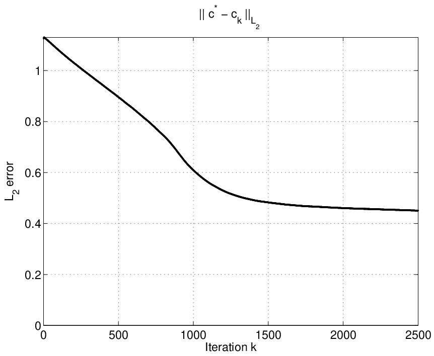
On the first run of the algorithm, see Figure 2 (a)–(c), the diffusion coefficient $a^{*}$ is assumed to be exactly known. In this situation, the level set method is able to identify the absorption coefficient (see Figure 2 (a) for the evolution of the iteration error), and the iteration stagnates after that. The corresponding differences between the exact solution $c^{*}$ and the initial guess $c_{0}$ and between the exact solution $c^{*}$ and the final iterate $c_{2500}$ are plotted in pictures (b) and (c) respectively.
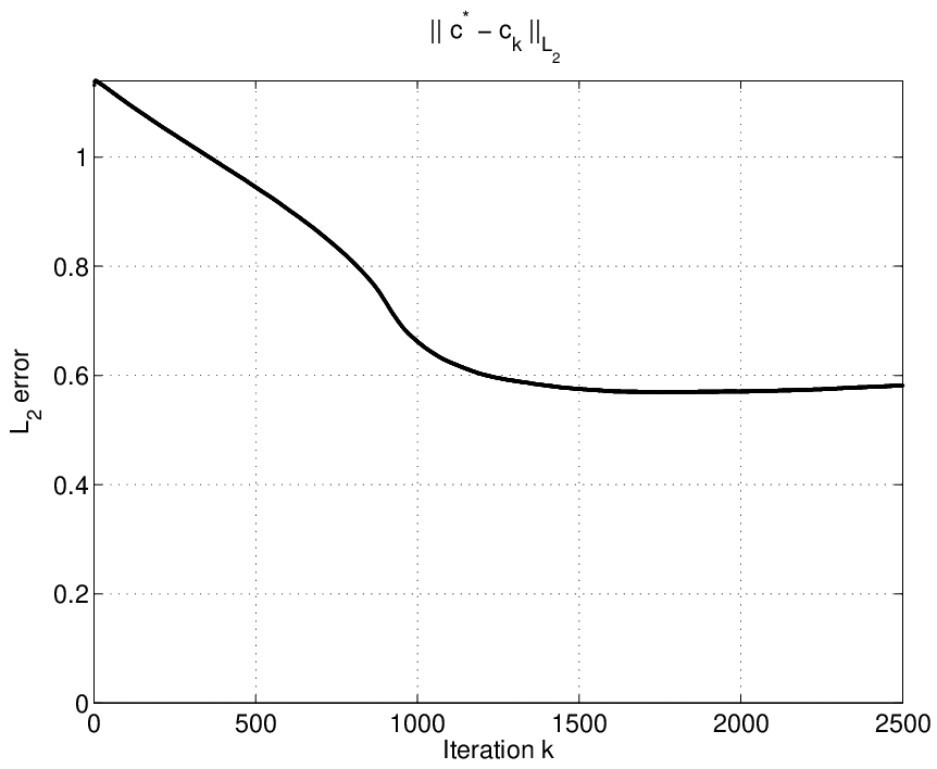
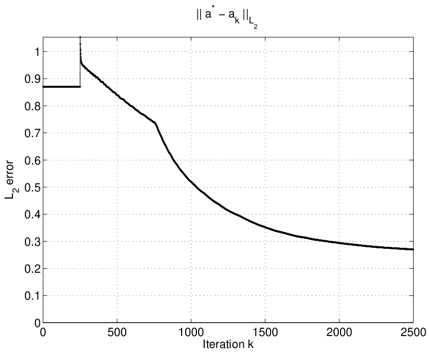
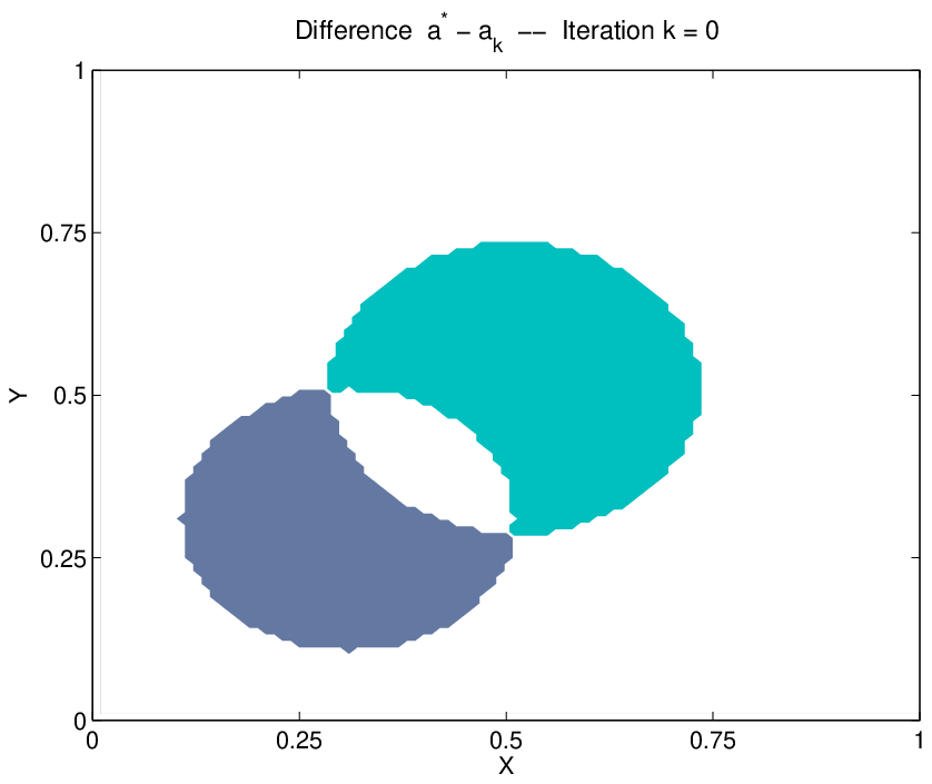
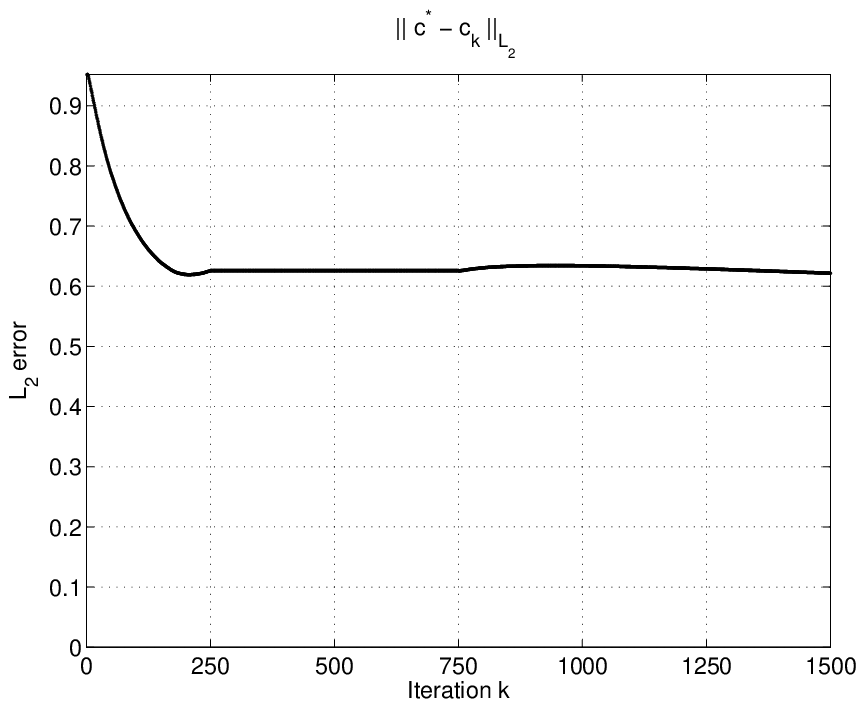
On the second run, see Figure 2 (d)–(f), we use the approximation $a(x)\equiv 1$ for diffusion coefficient $a^{*}$ and iterate to recover $c^{*}$ . In this case, the level set method is still able to identify the absorption coefficient, however with a poorer accuracy. Once again, the iteration stagnates after the numerical convergence is reached (see Figure 2 (d) for the evolution of the error). The corresponding differences for the initial guess $c_{0}$ and for the final iterate $c_{2500}$ are plotted in pictures (e) and (f) respectively.
Notice that the number of iteration steps needed to recover $c^{*}$ (approximately 2000 in both runs) is much larger than in the previous experiment. This can be explained by the complexity of the geometry of the support of $c^{*}$ in this experiment [15]. This complexity and non smooth geometry also influence the quality of the reconstruction.

5.2 Identification of the diffusion coefficient

In what follows we consider the identification of the diffusion coefficient $a$ , based on either total or partial knowledge of $c$ . In the first set of experiments, we consider problem (1)–(2) in the unit square with four pairs of NtD experiments, and the same exact solution $(a^{*},c^{*})$ as in Section 5.1 (see Figure 1 (a)).

As initial guess for the level set method we choose distinct piecewise constant functions $a_{0}$ , whose supports are shown in Figure 1 (c). Analogous as in Section 5.1, the constant values of the exact solution $a^{*}$ are assumed to be known, as well as the exact absorption coefficient $c^{*}$ . Moreover, exact data are used for the reconstruction (i.e., $\delta=0$ ) and the scaling factors $\beta_{j}=0$ .

This time, the inverse problem reduces to a shape identification problem for the diffusion coefficient. Once again we plot, for each initial guess $a_{0}$ , a corresponding number of steps (see Figure 1 (c)). It stands for the number of iterations needed to compute an approximation of $a^{*}$ (starting from the corresponding $a_{0}$ ) with a precision of $10^{-2}$ in the $L^{2}$ -norm.

This experiment allow us to determine the computational effort necessary for the reconstruction of $a^{*}$ with respect to distinct choices of $a_{0}$ . The identification problem for the diffusion coefficient is known to be exponentially ill-posed [13, 20]. This fact is in agreement with the values plotted in Figure 1 (c), meaning that the number of iterations necessary to achieve a good quality reconstruction does strongly oscillate with the initial guess.

We conduct yet another experiment for identifying only the diffusion coefficient. This time, we assume the exact solution of problem (1)–(2) to be given by the coefficient pair $(a^{*},c^{*})$ in Figure 1 (d). The setup of the inverse problem remains the same (domain, available data, parameter to output operator, etc.).
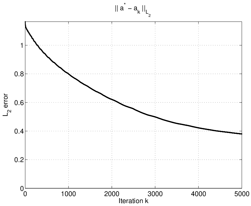
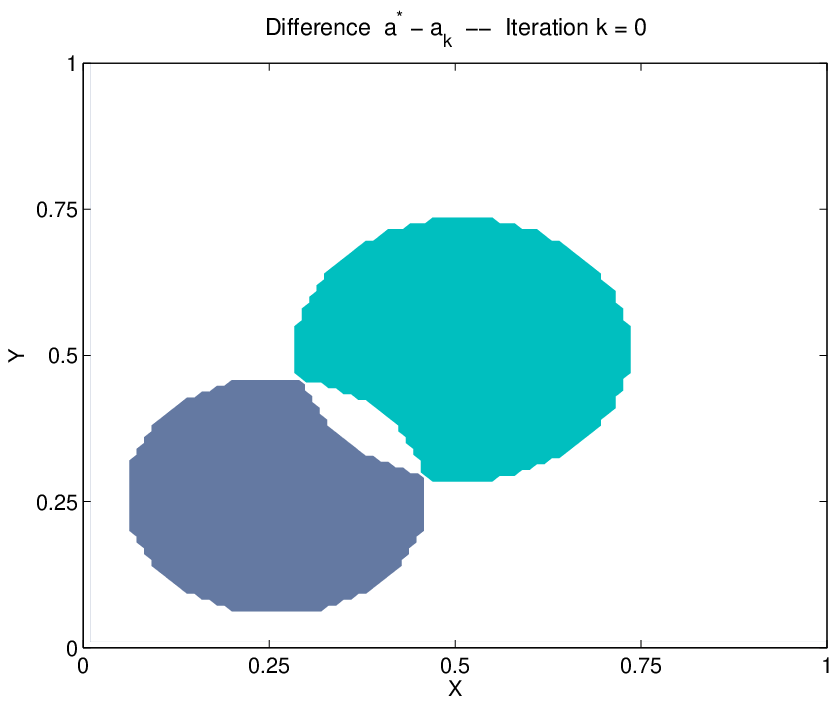
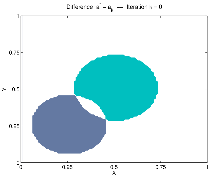
On the first run of the algorithm, see Figure 3 (a)–(c), the absorption coefficient $c^{*}$ is assumed to be exactly known. In this situation, the level set method is able to identify the diffusion coefficient (see Figure 3 (a) for the evolution of the iteration error), and the iteration stagnates after that. The corresponding differences between the exact solution $a^{*}$ and the initial guess $a_{0}$ and between the exact solution $a^{*}$ and the final iterate $a_{5000}$ are plotted in pictures (b) and (c) respectively.
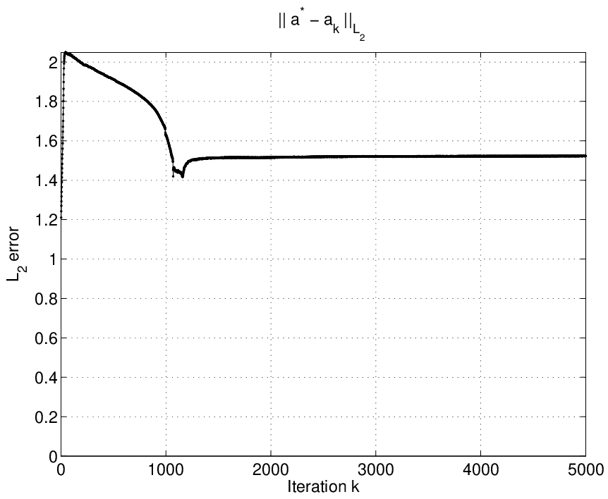
On the second run, see Figure 3 (d)–(f), we considered the approximation $\c{(}x)\equiv 1$ for the absorption coefficient $c^{*}$ and iterate to recover $a^{*}$ . In this case, the level set method is no longer able to identify the diffusion coefficient. The iteration once again stagnates, but this time at some configuration far from the exact solution (see Figure 3 (d) for the evolution of the $L^{2}$ error). The corresponding differences for the initial guess $a_{0}$ and for the final iterate $a_{5000}$ are plotted in pictures (e) and (f) respectively.

5.3 Identification of both diffusion and absorption coefficients

In this last set of experiments we consider the level set algorithm for the simultaneous identification of the coefficient pair $(a,c)$ in (1)–(2). Three examples are considered and the corresponding exact solutions are shown in Figure 4. The setup of the inverse problem is the same as in Sections 5.1 and 5.2 (domain, available data, parameter to output operator, …).

In the first example, the solution pair $(a^{*},c^{*})$ is the one shown in Figure 4 (a). In order to devise an efficient iteration strategy for the simultaneous identification of both coefficients, we must take some facts into account:
F1) From the 2nd example in Section 5.1, we have learned that the method for identifying $c^{*}$ performs well, even if a good approximation for $a^{*}$ is not known (see Figure 2 (d)–(f)).
F2) On the other hand, from the 2nd example in Section 5.2, we have learned that the level set method for identifying $a^{*}$ performs well if a good approximation for $c^{*}$ is available, but may generate a sequence $a_{k}$ that does not approximate $a^{*}$ if a good approximation to $c^{*}$ is not known.
F3) In the first run of the level set algorithm for the simultaneous identification of $(a^{*},c^{*})$ we updated both coefficients $(a_{k},c_{k})$ in every step and observed that the iteration error $\|c_{k}-c^{*}\|$ decreases from the very first iteration. However, the iteration error $\|a_{k}-a^{*}\|$ only starts improving when $\|c_{k}-c^{*}\|$ is sufficiently small.

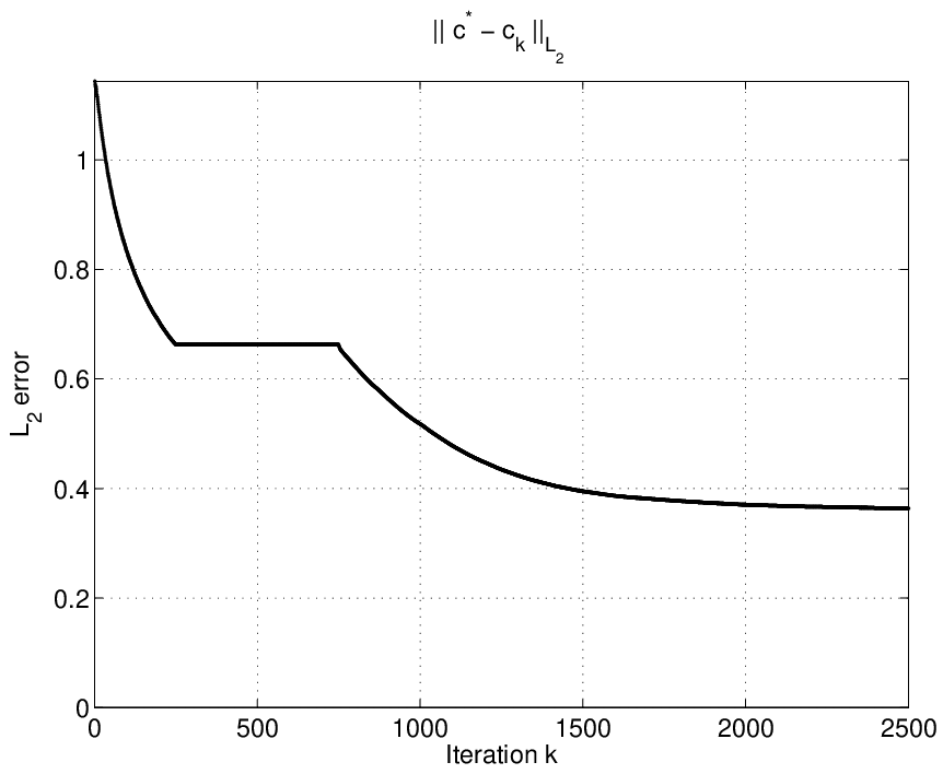
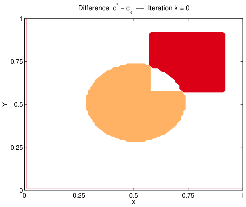
Thus, in order to save computational effort, we adopted the strategy to “freeze” the coefficient $a_{k}(x)=a_{0}(x)\equiv 1$ during the first iterations, and to iterate only with respect to $c_{k}$ . We follow this strategy until the sequence $c_{k}$ stagnates (this is an indication that the iteration error $\|c_{k}-c^{*}\|$ is small). In Figure 5 (a) and (e) this stage corresponds to the first $k_{1}=250$ iterative steps (notice that $\|a_{k}-a^{*}\|$ remains constant for $k=0,\dots,k_{1}$ , while the difference $c_{k_{1}}-c^{*}$ is plotted in (g)).

After this first iteration stage, we freeze $c_{k}=c_{k_{1}}$ and iterate only with respect to $a_{k}$ . This characterizes the second stage of the method. A natural question at this point would be: Why not to iterate with respect to both $(a_{k},c_{k})$ for $k\geq k_{1}$ ? We tried to proceed in this way, but what we observed is that: as long as $\|a_{k}-a^{*}\|$ does not significantly improve, the iterates $c_{k}$ stagnate with $\|c_{k}-c_{k_{1}}\|$ almost constant.
This second stage of the iteration can be observed in Figure 5 (a) and (e). Notice that $\|a_{k}-a^{*}\|$ decreases significantly, while $\|c_{k}-c^{*}\|$ remains constant for $k=k_{1},\dots,k_{2}=750$ (the difference $a_{k_{2}}-a^{*}$ is plotted in Figure 5 (c)).

After the conclusion of the second iteration stage, the pair $(a_{k},c_{k})$ is already a good approximation for $(a^{*},c^{*})$ (see Figure 5 (c) and (g)). As a matter of fact, this approximation is so good that, proceeding with the iteration simultaneously with respect to both $(a_{k},c_{k})$ , the iteration errors $\|a_{k}-a^{*}\|$ and $\|c_{k}-c^{*}\|$ are monotone decreasing. However, having in mind the convergence of the diffusion coefficient $a_{k}$ to the correct solution $a^{*}$ takes more iterations than the absorption coefficient $c_{k}$ , in this third stage we decided that each iteration step consists in one iteration with respect to the absorption coefficient $c_{k}$ and two iterations with respect to the diffusion coefficient $a_{k}$ (see Figure 5 (a) and (e) for $k\geq k_{2}$ ).

The introduction of this 3-stage iteration is motivated by the above mentioned facts (F1) – (F3). The calculation of optimal transition indexes $k_{1}$ , $k_{2}$ between the three stages is a difficult task. However, since the degree of ill-posedness of the separate inverse problems for $a$ and $c$ is very distinct from each other it’s not hard to get approximate values for $k_{1}$ and $k_{2}$ that will lead to a large gain in computational effort by using this 3-stage strategy.

The following second and third examples in this section do belong together. The corresponding exact solutions are shown in Figure 4 (b) and (c) respectively. Our goal is to investigate how the distance between the supports of the exact solution pair $(a^{*},c^{*})$ may interfere with the quality of the reconstruction of each single coefficient. In the second example there is a positive distance between the supports, while in the third example both supports overlap.

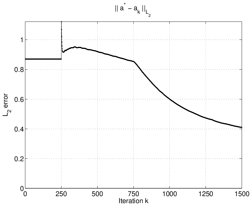
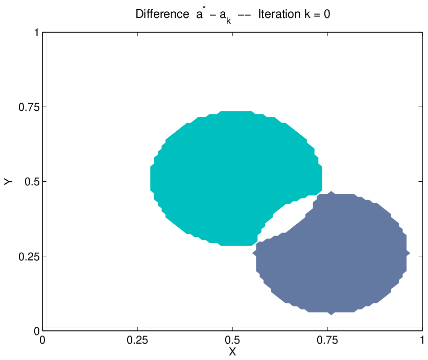
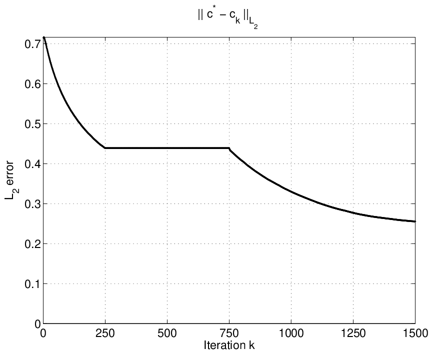
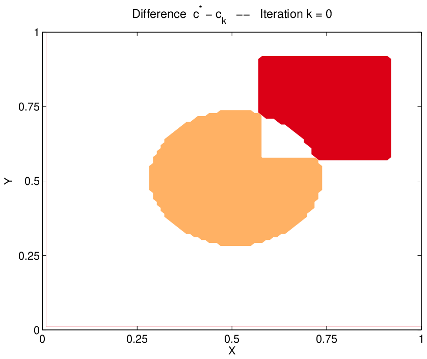
Although the distance between supp $(a^{*})$ and supp $(c^{*})$ in example 2 is smaller than in example 1 above, the 3-stage iteration behaves similarly in both examples. The 1st-stage is ended after $k_{1}=250$ iterations, when the error $\|c_{k}-c^{*}\|$ has decreased considerably (see Figure 6 (e)). The 2nd-stage corresponds to $k_{1}\leq k\leq k_{2}=750$ ; at this point the difference between the exact solution $a^{*}$ and the iteration $a_{750}$ has visibly decreased (see Figure 6 (c)). The 3rd-stage of the iteration corresponds to $k\geq k_{2}$ . In this final stage, each iteration step consists in two iterations with respect to the diffusion coefficient $a_{k}$ and one iteration with respect to the absorption coefficient $c_{k}$ . The final results can be observed in Figure 6 (d) and Figure 6 (h) respectively.

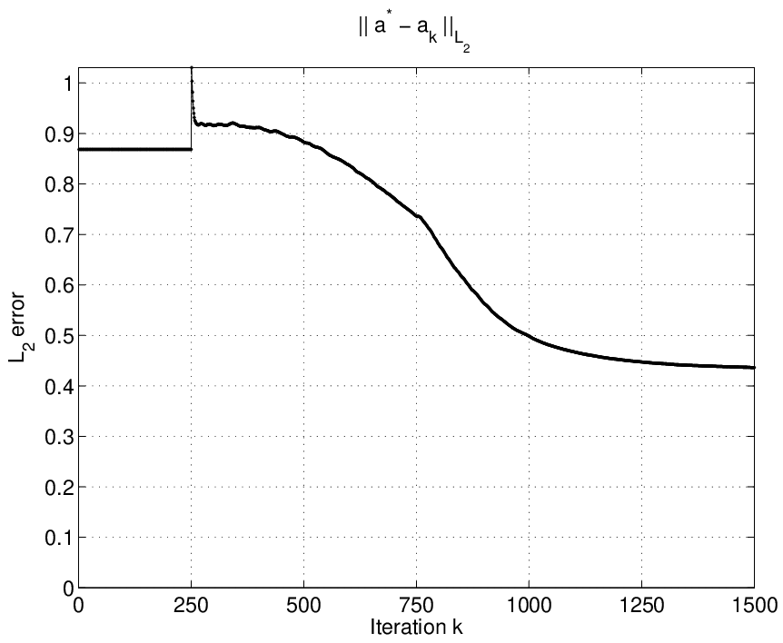
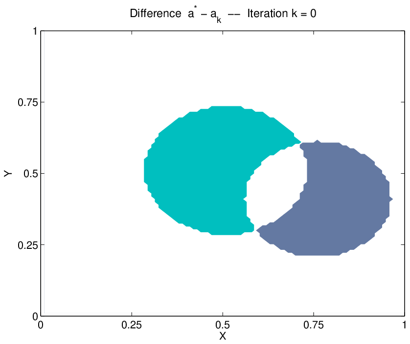
The third and last example reveled itself as the most difficult identification problem among all three considered in this section. The solution pair $(a^{*},c^{*})$ is chosen such that the supports of $a^{*}$ and $c^{*}$ intersect (see Figure 4 (c)). We start the iteration once again keeping $a_{k}$ constant during the first stage. This part of the method is successful, since after $k_{1}=500$ iterations $c_{k_{1}}$ delivers a good approximation for the exact solution $c^{*}$ (Figure 7 (g)). After that, we start iterating with respect to $a_{k}$ . After $k_{2}=750$ iterations we observe that the error $\|a_{k}-a^{*}\|$ has decreased considerably (Figure 7 (a)). Finally, we start with 3rd-stage of the algorithm and this is the point where the difficulties arise. No matter how many iterations we compute with respect to $c_{k}$ , the approximation does not get better than the one plotted in Figure 7 (g), which is computed after $k_{1}=250$ steps. After $1500$ steps, no significant improvement can be observed in the reconstruction of the absorption coefficient (compare Figure 7 (g) and (h)). In this last example, the reconstruction of the diffusion coefficient is very precise, but the approximation obtained for the absorption coefficient is not so good.

It is worth noticing that the poor reconstruction of $c^{*}$ is not due to non-stable behavior of our 3-stage algorithm. The particular exact solution $(a^{*},c^{*})$ in this example (with intersecting supports) leads to a very hard identification problem already reported in [31, 22, 3].

It is worth mentioning that all problems presented in this Section were solved using the standard level set method described in Section 3.2, i.e., updating both $(a_{k},c_{k})$ in every iterative step (and neglecting the 3-stage strategy). The final results of these iterations were basically the same as the ones presented here. However, the computational effort involved in the computation was by far much larger.

6 Conclusions

In this paper, we develop a level set regularization approach for simultaneous reconstruction of the piecewise constant coefficients $(a,c)$ from a finite set of boundary measurements of optical tomography in the diffusive regime. From the theoretical point of view, we prove that the forward map $F$ is continuous in the $[L^{1}(\Omega)]^{2}$ topology. Hence, following standard arguments presented by the authors in previous papers (see [8]) we get that the proposed level set strategy is a regularization method. The main result behind the continuity of $F$ is a generalization of Meyers’ Theorem for our particular case.

On the other hand, we propose a numerical algorithm to reconstruct simultaneously the diffusion and absorption coefficients. Both coefficients are computed by minimizing a regularized energy functional. Motivated by the fact that the reconstruction of the absorption coefficient $c$ is a mildly ill-posed inverse problem whereas the reconstruction of the diffusion coefficient $a$ is exponentially ill-posed, we present a split strategy that consists in freezing $a=a_{0}$ and first iterate with respect to $c$ until the iteration stagnate. Then, keep $c=c_{k}$ and start to iterate with respect to $a$ until stagnation of the iteration. Finally, iterate both coefficient. This numerical strategy has not only demonstrated that gives very good results but also reduces significantly the computational effort.

The situation of non-convergence of the level set algorithm, that is when coefficients $(a,c)$ have a crossing section (as in Subsection 5.3) is not an easy problem and it has already been reported in [31, 22, 3]. We conjecture that the level set algorithm will improve its performance if enough pairs of Neumann-to-Dirichlet data are available. Since the situation with many measurements is numerically demanding, a strategy like the one proposed in [25] could be more appropriated. We let this problem for future and careful investigation.

Acknowledgments

The work of J.P.A. was partially supported by grants from CONICET and SECY-UNC.

A.D. acknowledges support from CNPq - Science Without Border grant 200815/2012-1, ARD-FAPERGS grant 0839 12-3 and CNPq grant 472154/2013-3.

The work of M.M.A. was partially supported by CNPq grants no. 406250/2013-8, 237068/2013-3 and 306317/2014-1.

The authors would like to thanks Prof. Dr. Uri M. Ascher for the all discussions and valuable suggestions.

Appendix A Proof of Theorem 1

The main purpose of this appendix is to show that under mild assumptions on the boundary (Neumann) data $g$ the solution $u$ of (1)–(2) belongs to $W^{1,p}(\Omega)$ for some $p>2$ (therefore better than the standard regularity $u\in H^{1}(\Omega)$ ).

As far as we know, this type of regularity, namely $u\in W^{1,p}(\Omega)$ for $p>2$ , goes back to the pioneering work of Meyers [23], for elliptic BVPs with Dirichlet boundary conditions. Later on, Gallouet and Monier [16] generalized Meyers’ result to Neumann BVPs. However, for the best of the authors knowledge there is no proof of such a result for the problem (1)–(2).

The following proof was suggested by one of the anonymous referees. The authors are grateful to him for this suggestion.

Proof of Theorem 1

Let $u\in H^{1}(\Omega)$ be the unique solution of (1)–(2). It clearly satisfies the weak formulation

\displaystyle\int_{\Omega}a\nabla u\cdot\nabla\varphi dx+\int_{\Omega}cu\varphi dx=\int_{\Gamma}g\varphi d\sigma\qquad\forall\varphi\in H^{1}(\Omega).

(27)

Define now $\tilde{u}:=u-\dfrac{1}{|\Omega|}\int_{\Omega}udx$ , which in particular satisfies the weak formulation (5) in [16], i.e.,

\left\{\begin{aligned} &\tilde{u}\in H^{1}_{*}(\Omega),\\ &\int_{\Omega}a\nabla\tilde{u}\cdot\nabla\varphi dx=\langle f,\varphi\rangle_{(H^{1})^{\prime},H^{1}}\qquad\forall\varphi\in H^{1}(\Omega),\end{aligned}\right.

where $f$ is defined as

\langle f,\varphi\rangle_{(H^{1})^{\prime},H^{1}}:=\int_{\Gamma}g\varphi d\sigma-\int_{\Omega}cu\varphi dx\qquad\forall\varphi\in H^{1}(\Omega).

Note that $f$ naturally satisfies $\langle f,1\rangle_{(H^{1})^{\prime},H^{1}}=0$ . Hence, to finish the proof we only need to apply the regularity result given in [16, Theorem 2]. To this end, it remains to show that the distribution $f$ is in $W^{1,q}(\Omega)^{\prime}$ . As $g$ belongs to $W^{1-1/q,q}(\Gamma)^{\prime}$ the distribution $\varphi\mapsto\int_{\Gamma}g\varphi d\sigma$ is in $W^{1,q}(\Omega)^{\prime}$ thanks to the trace theorem in Sobolev spaces. Next we shall prove that the distribution $h:\varphi\mapsto\int_{\Omega}\,cu\varphi\,dx$ also belongs to $W^{1,q}(\Omega)^{\prime}$ . Consider first the case $N=2$ . In this case, since $q<2$ , we have the continuous embedding [4, Corollary 9.14] $W^{1,q}(\Omega)\hookrightarrow L^{q^{*}}(\Omega)$ , where $q^{*}=2q/(2-q)>2$ . Letting $s:=q^{*}/(q^{*}-1)$ be the conjugate of $q^{*}$ we have $s<2$ (because $q^{*}>2$ ) and, as a consequence, the continuous embedding [4] $H^{1}(\Omega)\hookrightarrow L^{2}(\Omega)\hookrightarrow L^{s}(\Omega)$ . Using the latter inclusions, the fact that $u\in H^{1}(\Omega)$ , the second inequality in (4) and the Hölder’s inequality, we obtain (for all $\varphi\in W^{1,q}(\Omega)$ ):

	$\displaystyle\left\|\langle h,\varphi\rangle\right\|=\left\|\int_{\Omega}\,c(x)u\varphi\,dx\right\|$	$\displaystyle\leq\overline{c}\\|u\\|_{L^{s}}\\|\varphi\\|_{L^{q^{*}}}$
		$\displaystyle\leq\overline{c}\\|u\\|_{L^{s}}\\|\varphi\\|_{W^{1,q}},$		(28)

which proves that $h\in W^{1,q}(\Omega)^{\prime}$ . Consider now the case $N\in\{3,4\}$ and let $q^{*}:=qN/(N-q)>1$ and (as before) $s:=q^{*}/(q^{*}-1)$ its conjugate. In this case, we have also the continuous embeddings [4, Corollary 9.14] $W^{1,q}(\Omega)\hookrightarrow L^{q^{*}}(\Omega)$ and, since $1\leq s\leq 2^{*}:=2N/(N-2)$ , $H^{1}(\Omega)\hookrightarrow L^{s}(\Omega)$ . Using the same reasoning as in the case $N=2$ we find that (28) also holds when $N\in\{3,4\}$ which concludes the proof of the desired regularity to the distribution $h$ . Altogether, we obtain that $f$ is well-defined and belongs to $W^{1,q}(\Omega)^{\prime}$ .

References

[1] S. R. Arridge. Optical tomography in medical imaging. Inverse Problems, 15(2):R41–R93, 1999.
[2] S. R. Arridge and W.R.B. Lionheart. Nonuniqueness in diffusion-based optical tomography. Opt. Lett., 23:882–4, 1998.
[3] S. R. Arridge and M. Schweiger. A general framework for iterative reconstruction algorithms in optical tomography, using a finite element method. In Computational radiology and imaging (Minneapolis, MN, 1997), volume 110 of IMA Vol. Math. Appl., pages 45–70. Springer, New York, 1999.
[4] Haim Brezis. Functional analysis, Sobolev spaces and partial differential equations. Universitext. Springer, New York, 2011.
[5] M. Burger and S. Osher. A survey on level set methods for inverse problems and optimal design. European J. Appl. Math., 16(2):263–301, 2005.
[6] R. Dautray and J.-L. Lions. Mathematical analysis and numerical methods for science and technology. Vol. 2. Springer-Verlag, Berlin, 1988.
[7] A. De Cezaro, A. Leitão, and X.-C. Tai. On level-set type methods for recovering piecewise constant solutions of ill-posed problems. In X.-C. Tai, K. Mørken, K. Lysaker, and K.-A. Lie, editors, Scale Space and Variational Methods in Computer Vision, volume 5667 of Lecture Notes in Comput. Sci., pages 50–62. Springer, Berlin, 2009.
[8] A. De Cezaro, A. Leitão, and X.-C. Tai. On multiple level-set regularization methods for inverse problems. Inverse Problems, 25:035004, 2009.
[9] A. De Cezaro, A. Leitão, and X.-C. Tai. On piecewise constant level-set (pcls) methods for the identication of discontinuous parameters in ill-posed problems. Inverse Problems, 29:015003, 2013.
[10] A. De Cezaro and A. Leitão. Level-set of ${L}^{2}$ type for recovering shape and contrast in inverse problems. Inverse Problems in Science and Enginnering, 20(4):517–587, 2012.
[11] A. De Cezaro and A. Leitão. Corrigendum: Level-set of ${L}^{2}$ type for recovering shape and contrast in inverse problems. Inverse Problems in Science and Enginnering, 21:1–2, 2013.
[12] O. Dorn and D. Lesselier. Level set methods for inverse scattering—some recent developments. Inverse Problems, 25(12):125001, 11, 2009.
[13] H. W. Engl, M. Hanke, and A. Neubauer. Regularization of inverse problems, volume 375 of Mathematics and its Applications. Kluwer Academic Publishers Group, Dordrecht, 1996.
[14] L.C. Evans and R.F. Gariepy. Measure theory and fine properties of functions. Studies in Advanced Mathematics. CRC Press, Boca Raton, FL, 1992.
[15] F. Frühauf, O. Scherzer, and A. Leitão. Analysis of regularization methods for the solution of ill-posed problems involving discontinuous operators. SIAM J. Numer. Anal., 43:767–786, 2005.
[16] T. Gallouet and A. Monier. On the regularity of solutions to elliptic equations. Rend. Mat. Appl. (7), 19(4):471–488 (2000), 1999.
[17] A. P. Gibson, J. C. Hebden, and S. R. Arridge. Recent advances in diffuse optical imaging. Physics in Medicine and Biology, 50(4):R1–R43, 2005.
[18] B. Harrach. On uniqueness in diffuse optical tomography. Inverse Problems, 25(5):055010, 14, 2009.
[19] Jeremy C Hebden, Simon R Arridge, and David T Delpy. Optical imaging in medicine: I. experimental techniques. Physics in Medicine and Biology, 42(5):825, 1997.
[20] V. Isakov. Inverse problems for partial differential equations, volume 127 of Applied Mathematical Sciences. Springer, New York, second edition, 2006.
[21] B. Kaltenbacher, A. Neubauer, and O. Scherzer. Iterative regularization methods for nonlinear ill-posed problems, volume 6 of Radon Series on Computational and Applied Mathematics. Walter de Gruyter GmbH & Co. KG, Berlin, 2008.
[22] V. Kolehmainen, S. R. Arridge, W. R. B. Lionheart, M. Vauhkonen, and J. P. Kaipio. Recovery of region boundaries of piecewise constant coefficients of an elliptic PDE from boundary data. Inverse Problems, 15(5):1375–1391, 1999.
[23] N. G. Meyers. An $L^{p}$ -estimate for the gradient of solutions of second order elliptic divergence equations. Ann. Scuola Norm. Sup. Pisa (3), 17:189–206, 1963.
[24] Vasilis Ntziachristos, XuHui Ma, A. G. Yodh, and Britton Chance. Multichannel photon counting instrument for spatially resolved near infrared spectroscopy. Review of Scientific Instruments, 70(1):193–201, 1999.
[25] F. Roosta-Khorasani, Kees van den Doel, and Uri M. Ascher. Stochastic algorithms for inverse problems involving pdes and many measurements. SIAM J. Scient. Comput., 36:s3–s22, 2014.
[26] F. Santosa. A level-set approach for inverse problems involving obstacles. ESAIM Contrôle Optim. Calc. Var., 1:17–33, 1995/96.
[27] M. Schweiger and S. R. Arridge. Application of temporal filters to time resolved data in optical tomography. Phys Med Biol., 44(7):1699–717, 1999.
[28] M. Schweiger, S. R. Arridge, M. Hiraoka, and D. T. Delpy. The finite element model for the propagation of light in scattering media: boundary and source conditions. Med. Phys., 22(11):1779–1792, 1995.
[29] T. Tarvainen, B.T. Cox, J.P. Kaipo, and S.R. Arridge. Reconstructing absorption and scattering distributions in quantitative photoacoustic tomography. Inverse Problems, 28:084009, 2012.
[30] K. van den Doel and U. M. Ascher. On level set regularization for highly ill-posed distributed parameter estimation problems. J. Comput. Phys., 216(2):707–723, 2006.
[31] Yong Xu, Xuejun Gu, Taufiquar Khan, and Huabei Jiang. Absorption and scattering images of heterogeneous scattering media can be simultaneously reconstructed by use of dc data. Appl. Opt., 41(25):5427–5437, 2002.
[32] A. D. Zacharopoulos, S.R. Arridge, O. Dorn, V. Kolehmainen, and J. Sikora. Three-dimensional reconstruction of shape and piecewise constant region values for optical tomography using spherical harmonic parametrization and a boundary element method. Inverse Problems, 22(5):1509–1532, 2006.

	$\displaystyle\min\{\underline{a},\underline{c}\}\\|w\\|^{2}_{H^{1}}$	$\displaystyle\leq\\|a^{\prime}-a\\|_{L^{s}}{\left\lVert\nabla u^{\prime}\right\rVert}_{L^{p}}{\left\lVert\nabla w\right\rVert}_{L^{2}}+\\|c^{\prime}-c\\|_{L^{s}}{\left\lVert u^{\prime}\right\rVert}_{L^{p}}{\left\lVert w\right\rVert}_{L^{2}}$
		$\displaystyle\leq\left(\\|a^{\prime}-a\\|_{L^{s}}{\left\lVert\nabla u^{\prime}\right\rVert}_{L^{p}}+\\|c^{\prime}-c\\|_{L^{s}}{\left\lVert u^{\prime}\right\rVert}_{L^{p}}\right){\left\lVert w\right\rVert}_{H^{1}}$
		$\displaystyle\leq 2\left(\max\{\overline{a}-\underline{a},\overline{c}-\underline{c}\}\right)^{(s-1)/s}{\left\lVert u^{\prime}\right\rVert}_{W^{1,p}}\left({\left\lVert a^{\prime}-a\right\rVert}_{L^{1}}+{\left\lVert c^{\prime}-c\right\rVert}_{L^{1}}\right)^{1/s}{\left\lVert w\right\rVert}_{H^{1}}.$

	$\displaystyle\left\|\langle h,\varphi\rangle\right\|=\left\|\int_{\Omega}\,c(x)u\varphi\,dx\right\|$	$\displaystyle\leq\overline{c}\\|u\\|_{L^{s}}\\|\varphi\\|_{L^{q^{*}}}$
		$\displaystyle\leq\overline{c}\\|u\\|_{L^{s}}\\|\varphi\\|_{W^{1,q}},$		(28)

On the identification of piecewise constant coefficients in optical diffusion tomography by level set

Abstract

1 Introduction

2 The Parameter to Measurement Map

Definition 1.

Remark 1.

Theorem 1 (Generalized Meyers’ Theorem).

Lemma 2.

Proof.

Theorem 3.

Proof.

3 The level set framework with a finite number of experiments

Remark 2.

3.1 Modeling the parameter space: The level set framework

Level set framework:

3.2 Level set regularization

The concept of generalized minimizers:

Definition 2.

3.3 Convergence analysis of the level set approach

Theorem 4.

Proof.

4 Numerical realization

Proposition 5.

Proof.

4.1 Optimality conditions for the Tikhonov functional 𝒢ε,α{\cal G}_{{\varepsilon},\alpha}

Remark 3.

5 Numerical Experiments

5.1 Identification of the absorption coefficient

5.2 Identification of the diffusion coefficient

5.3 Identification of both diffusion and absorption coefficients

6 Conclusions

Acknowledgments

Appendix A Proof of Theorem 1

Proof of Theorem 1

References

4.1 Optimality conditions for the Tikhonov functional ${\cal G}_{{\varepsilon},\alpha}$