Unambiguous Delay-Doppler Recovery from Random Phase Coded Pulses

In the signal model, a pulse-Doppler radar transceiver transmits a phase-coded pulse train consisting of $P$ equally spaced pulses. For $0\leq t\leq PT_{r}$, this pulse train is given by

where $h(t)$ is the time-limited baseband waveform taking nonzero values in the interval $[0,T_{h})$ (with $T_{h}$ being the pulse width), the pulse-to-pulse delay $T_{r}$ is the PRI, and $f_{c}$ is the carrier frequency. We use $\phi[p]$ to represent the phase shift of the $p$-th pulse, for $p=0,\ldots,P-1$. As opposed to the traditional pulse Doppler radar, where the phase codes are identical, here in the random phase coded pulse radar, $\phi[p]$ is randomly distributed in the interval $[0,2\pi)$ and varies from pulse to pulse. The entire span of the signal in (1) is called the coherent processing interval (CPI). We also assume that $h(t)$ is band-limited, and $B_{h}$ is referred to as the bandwidth of $h(t)$.

Consider that the radar illuminates a point target moving with radial velocity $V$, whose distance to the radar is given by $R(t)=R(0)-Vt$. The echo signal from the target is [20]

where $\tau(t)$ is the round-trip time delay and $\alpha$ is a complex amplitude factor accounting for the antenna gain, the two-way path loss and the target’s RCS. From [20], the time delay can be approximately given by

if $V\ll c$, where $\tau=2R(0)/c$. Combining (2) and (3),

where $\nu=-2Vf_{c}/c$ is defined as the Doppler frequency. In (4), the velocity stretches or compresses the envelop of the pulse train by the factor $1+2V/c$ [20]. When $V\ll c$, this effect is negligible, and the signal after down-conversion is

where $\alpha$ incorporates the factor $e^{-j2\pi f_{c}\tau}$.

Next we consider a target scene with $L$ point targets located within the radar coverage region. The $l$-th target is defined by three parameters: a time delay $\tilde{\tau}_{l}=2R_{l}/c$, where $R_{l}$ is the distance from the radar to the target at $t=0$; a Doppler frequency $\nu_{l}=2V_{l}/\lambda$, where $V_{l}$ is the radial velocity of the target; and a complex amplitude factor of the echo signal $\alpha_{l}$. The targets are assumed to have non-fluctuating RCSs, or have slowly-fluctuating RCSs, e.g. satisfying the Swerling-1 model [21, 10], and hence $\alpha_{l}$ is constant during the CPI. The targets are defined in the radar radial coordinate system and the Doppler frequencies are assumed to lie in the unambiguous frequency region, that is $\nu_{l}\in[0,1/T_{r})$, for $l=0,\ldots,L-1$. As opposed to the common assumption in traditional radars, the time delays $\tilde{\tau}_{l}$ are not assumed to lie in the unambiguous region, namely less than $T_{r}$, but may exceed $T_{r}$, and range ambiguity occurs for a conventional pulse Doppler radar. For convenience, we decompose $\tilde{\tau}_{l}$ into its integer part (the ambiguity order) $q_{l}$ and the fractional part (the folded or reduced delay) $\tau_{l}$ as

where $q_{l}\geq 0$ is an integer and $0\leq\tau_{l}<T_{r}$. Range ambiguity may occur in radars that have wide observation range and transmit pulses with high PRF for considerations such as: (a) avoiding Doppler ambiguity for high frequency radars; (b) increasing the integrated power for low peak power radars [22]; (c) increasing the data rate in joint radar-communication systems [23].

From (5), the received signal after down-converting is written as

where $u(t)$ is additive white Gaussian noise (AWGN) with variance $\sigma^{2}$. Under the reasonable assumption $\max_{l}|\nu_{l}|\ll 1/T_{h}$, $y(t)$ can be approximated as [20]

for $0\leq t\leq PT_{r}$, where $\tilde{\alpha}_{l}={\alpha}_{l}e^{-j2\pi\nu_{l}\tau_{l}}$.

For convenience, we rewrite the overall received signal in (8) with respect to each PRI. Note that in traditional pulse Doppler settings, namely under the assumption that $0\leq\tilde{\tau}_{l}<T_{r}$, the $p$-th pulse reflected from the targets is received in the $p$-th PRI. Here, the $p$-th pulse reflected from the $l$-th target is received in the $(p+q_{l})$-th PRI. Figure 1 illustrates this phenomenon for $q_{l}=1$, in which the $b$-th pulse is received in the $(b+1)$-th PRI. In other words, the $(b-q_{l})$-th pulse reflected from the $l$-th target is received in the $b$-th PRI. Substituting $p=b-q_{l}$, we can rewrite (8) as

for $0\leq t\leq PT_{r}$, where the sequence $\{z[p]\}$ is defined as

From (9), the received signal in the $b$-th PRI is expressed as

for $b=0,1,\dots,P-1$ and $bT_{r}\leq t<(b+1)T_{r}$.

Given the received signal $y_{b}(t)$, $b=0,\ldots,P-1$, our goal is to recover the range and velocity of targets, namely the time delays $\{\tilde{\tau}_{l}\}$ and Dopplers $\{\nu_{l}\}$, $l=0,\ldots,L-1$. To recover these parameters, we first sample the signal, as presented in the next subsection.

To reduce the sampling rates, we apply sub-Nyquist sampling in fast time, namely sampling the signal in each PRI with sampling rate lower than the bandwidth $B_{h}$. Generally, aliasing of frequency bands will occur if the sampling rate is below the signal bandwidth. Nevertheless, the proposed techniques for sub-Nyquist radar [15, 16, 17] can obtain the necessary frequency information to recover target parameters without aliasing, by appropriate analog anti-aliasing filtering before sub-Nyquist sampling.

To see this, we compute the Fourier series representation of the aligned received signal in the $b$-th PRI $y_{b}(t+bT_{r})$ with respect to the period $[0,T_{r})$. This results in [15, 16]

for $m=0,\ldots,N-1$, where $H(\cdot)$ denotes the Fourier transform of $h(t)$, $N=\lfloor B_{h}T_{r}\rfloor$ is the number of Fourier samples, and $\{U_{b}[m]\}$ are the Fourier coefficients of $u_{b}(t+bT_{r})$. Here, $\lfloor\cdot\rfloor$ represents the floor function. For convenience, let

be the normalized Fourier coefficients of the $b$-th PRI, where $\tilde{U}_{b}[m]=T_{r}U_{b}[m]/H(2\pi m/T_{r})$.

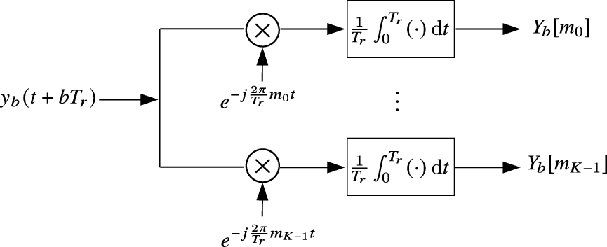
From (13), the target parameters $\{\tau_{l},\nu_{l},q_{l}\}$ are contained in the normalized Fourier coefficients $\tilde{Y}_{b}[k]$. To recover the target parameters, a sub-Nyquist radar obtains the Fourier coefficients from low rate samples of the received signal in each PRI. In this paper, we consider Xampling [24, 25] based sub-Nyquist radar systems. For each PRI, Xampling allows one to generate an arbitrary subset

comprised of $K=|\kappa|$ frequency components, and obtain the corresponding Fourier coefficients $Y_{b}[m_{k}]$, for $k=0,\ldots,K-1$, from $K$ point-wise samples of the received signal $y_{b}(t+bT_{r})$ after appropriate analog pre-processing. The procedure of Xampling is shown in Fig. 2, in which the received signal is split into $K=|\kappa|$ channels. In the $k$-th channel, Xampling obtains $Y_{b}[m_{k}]$ by first mixing $y_{b}(t+bT_{r})$ with the harmonic signal $e^{-j(2\pi/T_{r})m_{k}t}$ and then integrating over the aligned receive window $[0,T_{r})$.

By applying Xampling at radar receivers, we can reduce the sample rate without affecting the range resolution if radar targets can be sparsely represented. Thus, the cost and complexity of the analog to digital converter (ADC) at radar receivers may be reduced, especially for wide-band radars.

After sub-Nyquist sampling, the problem is to recover the targets’ delays $\{\hat{\tau}_{l}\}$ and Dopplers $\{\nu_{l}\}$, from the compressed normalized Fourier series

for $b=0,\ldots,P-1$ and $k=0,\ldots,K-1$. We note that these Fourier series can also be obtained by conventional Nyquist sampling, if we implement the integration in Fig. 2 by performing a discrete Fourier transform to the samples. Therefore, the signal model in (14) holds in both Nyquist and sub-Nyquist regimes. Unlike sub-Nyquist sampling, in Nyquist sampling all the Fourier coefficient are obtained, i.e. $K=N$ and $m_{k}=k$, for $k=0,\ldots,N-1$.

In this subsection, we recast (14) in matrix form. To that aim, we assume that the delays and Dopplers of the $L$ targets lie on the center of delay resolution bins and Doppler resolution bins, respectively. As in traditional pulse Doppler radar, the size of a delay resolution bin is $T_{r}/N$, while that of a Doppler resolution bin is $1/(PT_{r})$. Then the delays and Doppler can be represented by $\tau_{l}=n_{l}T_{r}/N$ and $\nu_{l}=p_{l}/(PT_{r})$, where $n_{l}$ and $p_{l}$ are integers in the intervals $[0,N-1]$ and $[0,P-1]$, respectively, for $l=0,\ldots,L-1$. Under this assumption, (14) becomes

for $b=0,\ldots,P-1$ and $k=0,\ldots,K-1$.

Define the ambiguity factor

When $Q=1$, there is no range ambiguity. In our model, range ambiguity is considered, i.e. $Q>1$. In (15), the target parameters $\{\tilde{\alpha}_{l},n_{l},q_{l},p_{l}\}$ can be characterized by a matrix $\tilde{\bm{X}}\in\mathbb{C}^{N\times PQ}$, which is defined as

In other words, the matrix $\tilde{\bm{X}}$ is an $N\times PQ$ matrix which contains the value $\tilde{\alpha}_{l}$ at the corresponding $L$ indexes $(n_{l},Pq_{l}+p_{l})$, for $l=0,\ldots,L-1$, while the rest of the elements in $\tilde{\bm{X}}$ are all zeros.

We may now reformulate (15) into a matrix observation model

where the $(k,b)$-th entry of $\bm{Y}\in\mathbb{C}^{K\times P}$ is given by $\tilde{Y}_{b}[m_{k}]$, denoting the $k$-th Fourier coefficients of the radar signal received in the $b$-th PRI, for $b=0,\ldots,P-1$ and $k=0,\ldots,K-1$; the partial Fourier matrix $\bm{A}\in\mathbb{C}^{K\times N}$ has the $(k,n)$-th entry given by $W_{N}^{nm_{k}}$, representing the fast-time frequency response from the $n$-th range resolution bin at the frequency point $m_{k}/T_{r}$, for $n=0,\ldots,N-1$ and $k=0,\ldots,K-1$; and $\bm{U}\in\mathbb{C}^{K\times P}$ is the additive noise whose $(k,b)$-th entry is given by $\tilde{U}_{b}[m_{k}]$.

In (18), the matrix $\bm{B}\in\mathbb{C}^{P\times PQ}$ consists of $Q$ blocks. Particularly, $\bm{B}$ is represented by

where $\bm{B}^{(q)}\in\mathbb{C}^{P\times P}$, and the $(b,p)$-th entry of $\bm{B}^{(q)}$ is given by $W_{P}^{bp}z[b-q]$, for $p=0,\ldots,P-1$ and $b=0,\ldots,P-1$. Here, each block $\bm{B}^{(q)}$ represents the slow-time response of the targets with ambiguity order $q$.

From the matrix formation model (18), $\tilde{\bm{X}}$ should be a solution of the following equation

in the noiseless case. The problem is to recover the sparse matrix $\tilde{\bm{X}}$ from the observation $\bm{Y}$ and measurement matrix $\bm{A}$ and $\bm{B}$, by finding the solution of (20). For a Nyquist pulse-Doppler radar without range ambiguity, namely $K=N$ and $Q=1$, $\bm{A}$ and $\bm{B}$ are full-rank square matrices, so the solution to (20) is unique. However, in our setting, namely $K\leq N$ and $Q>1$, due to the rank deficiency of $\bm{A}$ and $\bm{B}$, (20) is an under-determined equation and may not have a unique solution.

Nevertheless, when $L\ll NPQ$, there are only a few nonzero elements in $\tilde{\bm{X}}$, which means that $\tilde{\bm{X}}$ is a sparse matrix. This sparsity of radar targets motivates the use of CS algorithms to solve the under-determined radar observation model. In recent years, CS algorithms have been applied to many fields of radars, such as synthetic aperture radar imaging [26, 27], space-time adaptive processing [28] and randomized stepped frequency radars [29, 30] and exhibit enhanced target reconstruction quality compared to a matched filter on real radar data [31, 30, 27]. In addition, various low complexity methods [32, 31] are proposed for the real-time implementation of CS algorithms on radars. In our problem, CS algorithms may be applicable for ground-to-air radars, where the sparsity of targets holds and the computation complexity of CS algorithms is affordable. We follow the concepts of CS and use sparse matrix recovery to recover $\tilde{\bm{X}}$ from the received signal, as discussed in the following section.

To derive the recovery conditions, we equivalently rewrite $\bm{Y}=\bm{A}\bm{X}\bm{B}^{\mathrm{T}}$ in vector form as [42]

where the operator $\mathrm{vec}(\cdot)$ produces a vector by stacking columns of a given matrix and $\otimes$ represents the Kronecker product. Correspondingly, the $\ell_{0}$ minimization problem (21) becomes

by letting $\bm{x}=\mathrm{vec}(\bm{X})$, $\bm{y}=\mathrm{vec}(\bm{Y})$ and

in (21). Let $\tilde{\bm{x}}=\mathrm{vec}(\tilde{\bm{X}})$. To unambiguously recover $\tilde{\bm{X}}$, we need $\tilde{\bm{x}}$ be the unique optimum of (23).

CS theory provides conditions for recovering $\tilde{\bm{x}}$ with (23) by investigating the spark property of the measurement matrix $\bm{T}$. The spark of $\bm{T}$ is defined as the size of the smallest linearly dependent subset of columns, i.e.

From the definition of spark, $\tilde{\bm{x}}$ is the unique optimum of (23) if $\mathrm{spark}(\bm{T})>2\|\tilde{\bm{x}}\|_{0}$ [43, 44]. From [42], one has that for $\bm{T}$ of (25),

Since $\|\tilde{\bm{x}}\|_{0}=\|\tilde{\bm{X}}\|_{0}=L$, the unambiguous recovery condition becomes

For convenience, let $\beta_{A}=\mathrm{spark}(\bm{A})$ and $\beta_{B}=\mathrm{spark}(\bm{B})$. A naive bound of $\beta_{A}$ is given by

because $\bm{A}$ is a $K\times N$ matrix with $K\leq N$ and any $K+1$ columns of $\bm{A}$ are linearly dependent. We observe that the last block in $\bm{B}$ only has $P-Q+1$ non-zero rows, meaning that any $P-Q+2$ columns from the last block are linearly dependent. As a result,

Since $\bm{A}$ is a partial Fourier matrix generated by selecting $K$ rows from a $N$-dimensional Fourier matrix indexed with the subset $\kappa\subset\left\{0,\ldots,N-1\right\}$, $\beta_{A}$ depends on $\kappa$. From [19, 45, 46], we can easily generate subsets $\kappa$ to ensure that $\bm{A}$ has full spark, i.e. $\beta_{A}=K+1$. We note that when the received signal is sampled at the Nyquist rate, i.e. $K=N$ and $\kappa=\left\{0,\ldots,N-1\right\}$, $\bm{A}$ becomes a full Fourier matrix and the $N$ columns of $\bm{A}$ are linearly independent. In this case, $\beta_{A}=N+1=K+1$.

Next, we note that $\bm{B}$ is a random matrix since each element in $\bm{B}$ includes a random phase item. Thus $\beta_{B}$ is a random variable with respect to $\{z[p]\}$. Under the assumption that the random phase item $\phi[p]$ is generated from a uniform distribution over $[0,2\pi)$, the spark of $\bm{B}$, $\beta_{B}$, almost surely equals $P-Q+2$, as indicated in the following theorem.

Combining the results on $\beta_{A}$ and $\beta_{B}$ with the recovery condition (27), we obtain the following theorem. In (30), $K$ is the number of samples in each PRI, $P$ is the number of transmit pulses and $Q$ is the ambiguity factor defined in (16).

The randomness of the phase codes $\{z[k]\}$ is crucial for the derivation of Theorem 1 and 2. In a pulse-Doppler radar without phase coding in which $z[0]=\cdots=z[P-1]$, it can be validated that

which means there exist $4$ linearly dependent columns in $\bm{B}$. As a consequence, $\beta_{B}\leq 4$ and the number of targets is bounded by $L<2$ from (27).

In the Nyquist regime, $\bm{A}$ is an invertible Fourier matrix. Therefore, (21) becomes

Let $\bm{X}^{\mathrm{T}}=[\bm{x}_{0},\ldots,\bm{x}_{N-1}]$. The problem in (33) can be split into multiple independent sub-problems:

for $n=0,\ldots,N-1$. The corresponding recovery condition for these sub-problems are

The conditions in the Nyquist regime only require that the number of targets within each reduced range resolution bin is bounded by $(P-Q+2)/2$, and is much looser than that in the sub-Nyquist regime, in which the total number of targets is bounded by $(P-Q+2)/2$.

We note that the upper bound on the number of targets in (35) is reduced compared to a conventional pulse Doppler radar. For a Nyquist pulse Doppler radar without range ambiguity, the matrix $\bm{B}$ becomes an invertible Fourier matrix. Thus, the targets can be recovered by directly solving (20) without using CS. Under this circumstance, the number of recoverable targets in each range resolution bin is $P$. In our setting, range ambiguity leads to rank deficiency of $\bm{B}$. As a result, the observation equation is under-determined, and is solved by sparse matrix recovery methods, for which the upper bound of the number of targets is given in (35).

We consider a pulse Doppler radar transmitting a pulse train composed of $P=20$ pulses with PRI $T_{r}=25\mu\mathrm{sec}$ over a CPI of $500\mu\mathrm{sec}$. The carrier frequency is $f_{c}=10\mathrm{GHz}$ and the propagation velocity is $f_{c}=3\times 10^{8}\mathrm{m/s}$. Then we have $R_{\mathrm{max}}=3.75\mathrm{km}$ and $V_{\mathrm{max}}=300\mathrm{m/s}$. The baseband waveform $h(t)$ is a linear frequency modulation pulse with bandwidth $B_{h}=20\mathrm{MHz}$ and pulse width $T_{h}=1\mu\mathrm{sec}$. Specifically, the expression of $h(t)$ is

To extend the maximal unambiguous range, we adopt range phase coding to each pulse, where the phase $\phi[p]$ is uniformly distributed in $[0,2\pi)$, for $p=0,\ldots,P-1$.

The number of Nyquist rate samples in each PRI is $N=T_{r}B_{h}=500$. In the simulations, we investigate sub-Nyquist sampling by reducing the number of samples $K$ in each PRI. We randomly select $K<N$ frequency components and obtain the corresponding compressed Fourier coefficients by the Xampling scheme in Fig. 2. We find that the matrix $\bm{A}$ has full-rank with high probability if the frequency components are selected randomly.

We consider $L$ targets with Doppler frequencies spread uniformly at random in the appropriate unambiguous region $\left[0,1/T_{r}\right)$ and delays spread uniformly at random in the ambiguous region $\left[0,QT_{r}\right)$ for ambiguity factor $Q$. In the simulations, the echoes from all targets have unit amplitude, i.e. $|\alpha_{l}|=1$, for $l=0,\ldots,L-1$.

In the simulations, we produce the received signal $y(t)$ with (7). The received signal is corrupted with AWGN $u(t)$ which has variance $\sigma^{2}$ and is band-limited to $B_{h}$. The total transmit SNR of the transmitted pulse train is

Here, the inter-pulse random phase coding does not affect the SNR after coherent integration.

After $y(t)$ is produced, we compute $Y_{b}[m]$ and $H(2\pi m/T_{r})$ by applying Fourier transform to $y_{b}(t)$ and $h(t)$, respectively. Then the elements of matrix $\bm{Y}$ are computed via (13) and (14), after which the delays and Dopplers of the targets are recovered by solving (21) via matrix OMP. We use a hit-or-miss criterion as a performance metric. A “hit” is defined as a delay-Doppler estimate circumscribed by a rectangles around the true target position in the time-frequency plane. We use rectangles with axes equivalent to $\pm 1$ times the delay and Doppler resolution bins, equal to $1/B_{h}=50\mathrm{nsec}$ and $1/(PT_{r})=2\mathrm{KHz}$, respectively.

We compare our approach to the popular MPRF method of [11] that has been shown to outperform the matching interval scheme based on the Chinese Remainder Theorem. In MPRF, the pulse Doppler radar transmits two pulse trains with baseband signal $h(t)$. The first train is composed of $P_{1}=20$ pulses, with PRI $T_{r,1}=25\mu\mathrm{sec}$ over a CPI of $500\mu\mathrm{sec}$. The second train is composed of $P_{2}=25$ pulses, with PRI $T_{r,2}=20\mu\mathrm{sec}$ over a CPI of $500\mathrm{\mu sec}$. Like the random phase coded pulses, the observation model in (18) still holds for each pulse train in the MPRF scheme, where the measurement matrix $\bm{B}$ is constructed for $Q=1$ and all $z[p]=1$. We use matrix OMP to recover the ambiguous delay-Doppler map from each pulse train. Once the targets’ Doppler frequencies and ambiguous delays are recovered, we apply the clustering method in [11] to estimate the unambiguous delays. The total transmit SNR of the two transmit pulse trains is

In this experiment, the number of targets is $L=5$ and ambiguity factor $Q=4$. Here, we require the Dopplers and delays lie in the center of Doppler and range resolution bins, respectively. Performance of RPPC and MPRF is compared with the same range resolution, Doppler resolution and total transmit SNR so that the comparison is fair.

Figure 3 presents the delay-Doppler recovery performance of both MPRF and RPPC with respect to transmit SNR. The results are obtained in both Nyquist and sub-Nyquist regimes. In the sub-Nyquist regime, we randomly choose $K=250$ and $K=125$ Fourier coefficients in each PRI, leading to a compression ratio of $50\%$ and $25\%$, respectively. As Fig. 3 shows, the hit rate increases with the increase of the total transmit SNR, which is proportional to the SNR after matched filtering in fast and slow time. We observe that our RPPC approach outperforms the MPRF approach in both Nyquist and sub-Nyquist regimes, in terms of the hit rate under the same total transmit SNR. The explanation is that the RPPC approach jointly processes all the received samples, while the MPRF approach processes the received samples of the two pulse trains separately. Therefore, the RPPC approaches can obtain better SNR after fast and slow time matched filter with the same total transmit SNR.

To achieve the same hit rate as MPRF, our RPPC technique requires a lower total transmit SNR, leading to around $3$dB SNR gain. As a result, for a radar transmit system with fixed pulse width, peak power and PRF, RPPC needs a lower number of transmit pulses to achieve a commensurate performance with MPRF, and thus reduces the cost of power and transmit time.

The impact of sub-Nyquist sampling is also demonstrated in Fig. 3. It is observed that the recovery performance in the Nyquist regime is better than that in the sub-Nyquist regime, and the recovery performance in sub-Nyquist regime decreases as the number of samples decreases. This is because sub-Nyquist sampling leads to loss of SNR.

The last experiment was conducted in the on-grid case, namely the delays and Dopplers lie in the center of the resolution bins. In this experiment, we consider a more realistic scene where the delays and Dopplers do not necessarily lie in the center of resolution bins, and examine the performance of matrix OMP in the off-grid case. In particular, there are $L=5$ point targets whose Doppler frequencies and delays can be arbitrary values in the region $\left[0,1/T_{r}\right)$ and $\left[0,QT_{r}\right)$ for $Q=4$, respectively.

In the off-grid case, we directly produce the Fourier coefficients in (12) for convenience. The hit rate of matrix OMP is computed for over-discretization factor $\gamma=1,2,4,16$. When $\gamma=1$, there is no over-discretization, i.e. the range and Doppler grid size are equal to the range and Doppler resolution, respectively. The result for Nyquist and sub-Nyquist sampling is given in Fig. 4 and Fig. 5, respectively. In the sub-Nyquist regime, we randomly choose $K=250$ Fourier coefficients in each PRI, leading to a compression ratio of $50\%$. The hit rate of matrix OMP in the on-grid case is also displayed for comparison. From Fig. 4 and Fig. 5, matrix OMP exhibits a serious performance degradation in the off-grid case compared to the on-grid case, if no over-discretization is performed. It it observed that the hit rate is only around $0.7$ even when the SNR is high enough because of the mismatch of observation model. Nevertheless, the performance degradation can be significantly relieved by over-discretization. When $\gamma\geq 2$, performance of matrix OMP in the off-grid case is still worse than the counterpart in the on-grid case, but the performance gap is not significant, especially when $\gamma$ is large. For a high SNR, the performance loss can be effectively reduced by increasing $\gamma$. The results here indicate that matrix OMP is still applicable in our problem by properly decreasing the grid size.

We also performed simulations to examine the impact of number of targets on the recovery performance. Specifically, the hit rate versus SNR is calculated and demonstrated in Fig. 6 for $L=7,9,11$, in both Nyquist and sub-Nyquist regimes, where $Q=4$ and the targets lie in the center of range-Doppler resolution bins. In the sub-Nyquist regime, we randomly choose $K=250$ Fourier coefficients in each PRI, leading to a compression ratio of $50\%$. It is observed that the recovery performance only slightly decreases as $L$ increases for both Nyquist and sub-Nyquist sampling if $L$ is not very large. Note that from the recovery condition obtained in Sec. IV-A for sub-Nyquist sampling, perfect recovery is guaranteed for arbitrary sparse matrix $\bm{X}$ with $L<9$. That means if $L<9$, the targets can always be recovered in the noise-less case, regardless of their locations and RCSs, while if $L\geq 9$, the targets may not be correctly reconstructed, depending on their parameters. Nevertheless, as shown in Fig. 6, the targets can still be recovered with a high probability when the targets are uniformly distributed, even if $L\geq 9$, namely the sparse recovery condition is not met. This result suggests that the sparsity constraint to radar targets can be relaxed in practical use, extending the application scope of sub-Nyquist sampling.

When the recovery condition is not met, although the ranges and Dopplers of randomly distributed targets may still be recovered with high probability, there should exist some radar target scenes in which recovery fails. Moreover, even if the recovery condition is met, the targets may not be perfectly recovered with practical algorithms like OMP and $\ell_{1}$ norm minimization. To show this, consider the worst case in which all the $L$ targets are located in the same reduced range resolution bin, i.e.

The velocities are uniformly distributed in the unambiguous region $[0,1/T_{r})$. The ambiguity orders can be arbitrary integers in $[0,Q-1]$. The delays and Dopplers of targets lie at the center of the corresponding resolution bins.

From the recovery condition, if $L<(P-Q+2)/2$, the targets can be recovered with probability 1 by finding the sparsest solution of (20). However, as practical algorithms may not find the sparsest solution, the hit rate for them may be less than $1$. Here, we evaluate the impact of the number of users on the hit rate under this target scene for $\ell_{1}$ norm minimization and OMP, under random pulse phase and random locations of targets. The simulation is run in the noiseless case and in the Nyquist regime. In particular, we recover $\bm{X}$ by solving the sub-problems in (34) via $\ell_{1}$ norm minimization and OMP. To reduce the computational complexity, we first detect the reduced range resolution bin where the targets lie, and then solve the sub-problem in the detected reduced range resolution bin.

The hit rate of versus number of users for $\ell_{1}$ norm minimization is given in Fig. 7, for different $Q$ and $P$. In Fig. 7, if $Q=1$, namely there is no range ambiguity, the hit rate is always 1 regardless of the number of targets, since the equation in (20) well-determined. If $Q>1$, the hit rate is close to 1 for small $L$, i.e. range ambiguity can be resolved for sparse targets. When $L$ becomes larger, the targets are not sparse enough and the hit rate can be rather low. From Fig. 7, it is observed that the number of recoverable targets can be increased by transmitting more pulses or reducing the ambiguity order. This observation is also verified by the theoretical bound $(P-Q+2)/2$. It is also observed that, to achieve a hit rate close to 1, the maximal number of recoverable targets with $\ell_{1}$ norm minimization is less than the theoretical bound, indicating the performance gap between $\ell_{1}$ norm minimization and $\ell_{0}$ minimization.

The hit rate of versus number of users for OMP is given in Fig. 8, for different $Q$ and $P$. Comparing Fig. 7 and 8, the recovery performance of OMP is worse than $\ell_{1}$ norm minimization although OMP generally has lower computation load. Nevertheless, OMP still guartantees a high hit rate when the number of targets is small.

In the end, we compare the computation time of matrix OMP under different number of targets. This comparison is performed for different $P$, in both Nyquist and sub-Nyquist regimes. In sub-Nyquist sampling, we randomly choose $K=250$ Fourier coefficients, leading to a compression ratio of $50\%$. The average computation time versus $L$ is shown in Fig. 9. From Fig. 9, we observe that the computation time of matrix OMP approximately grows linearly with $L$ when $L$ is small. When more pulses are transmitted, namely $P$ becomes larger, the computation load becomes higher. The computation time in the sub-Nuquist regime is less than the counterpart in the Nyquist regime, since sub-Nyquist sampling reduces the size of data.

References

- [1] R. J. Doviak and D. S. Zrnić, Doppler Radar and Weather Observations. Academic Press, 2014.
- [2] V. N. Bringi and V. Chandrasekar, Polarimetric Doppler Weather Radar: principles and applications. Cambridge University Press, 2005.
- [3] A. Ferrari, C. Berenguer, and G. Alengrin, “Doppler ambiguity resolution using multiple PRF,” IEEE Transactions on Aerospace and Electronic Systems, vol. 33, no. 3, pp. 738–751, July 1997.
- [4] V. Venkatesh, L. Li, M. McLinden, G. Heymsfield, and M. Coon, “A frequency diversity pulse-pair algorithm for extending Doppler radar velocity Nyquist range,” in 2016 IEEE Radar Conference (RadarConf), May 2016, pp. 1–6.
- [5] A. Ludloff, N. Füchter, F. Hagedorn, M. Minker, and H. Rohling, Doppler Processing, Waveform Design and Performance Measures for Some Pulsed Doppler and MTD-radars, ser. AEG-Telefunken Radaranlagen. AEG-Telefunken, 1981.
- [6] M. Richards, Fundamentals of Radar Signal Processing, ser. Professional Engineering. Mcgraw-hill, 2005.
- [7] G. M. Cleetus, “Properties of staggered PRF radar spectral components,” IEEE Transactions on Aerospace and Electronic Systems, vol. AES-12, no. 6, pp. 800–803, Nov 1976.
- [8] A. Ferrari, G. Alengrin, and C. Theys, “Doppler ambiguity resolution using staggered PRF with a new chirp sweep-rate estimation algorithm,” IEE Proceedings - Radar, Sonar and Navigation, vol. 142, no. 4, pp. 191–194, Aug 1995.
- [9] A. Ludloff and M. Minker, “Reliability of velocity measurement by MTD radar,” IEEE Transactions on Aerospace and Electronic Systems, vol. AES-21, no. 4, pp. 522–528, July 1985.
- [10] M. Skolnik, Radar Handbook, Third Edition. McGraw-Hill Education, 2008.
- [11] G. Trunk and S. Brockett, “Range and velocity ambiguity resolution,” in The Record of the 1993 IEEE National Radar Conference, 1993, pp. 146–149.
- [12] Q. Cao, G. Zhang, R. D. Palmer, and L. Lei, “Detection and mitigation of second-trip echo in polarimetric weather radar employing random phase coding,” IEEE Transactions on Geoscience and Remote Sensing, vol. 50, no. 4, pp. 1240–1253, April 2012.
- [13] T. Wimalajeewa, Y. C. Eldar, and P. K. Varshney, “Recovery of Sparse Matrices via Matrix Sketching,” ArXiv e-prints, Nov. 2013.
- [14] J. A. Tropp and A. C. Gilbert, “Signal recovery from random measurements via orthogonal matching pursuit,” IEEE Transactions on Information Theory, vol. 53, no. 12, pp. 4655–4666, Dec 2007.
- [15] O. Bar-Ilan and Y. C. Eldar, “Sub-Nyquist radar via Doppler focusing,” IEEE Transactions on Signal Processing, vol. 62, no. 7, pp. 1796–1811, April 2014.
- [16] E. Baransky, G. Itzhak, N. Wagner, I. Shmuel, E. Shoshan, and Y. C. Eldar, “Sub-Nyquist radar prototype: hardware and algorithm,” IEEE Transactions on Aerospace and Electronic Systems, vol. 50, no. 2, pp. 809–822, April 2014.
- [17] D. Cohen and Y. C. Eldar, “Sub-Nyquist radar systems: Temporal, spectral, and spatial compression,” IEEE Signal Processing Magazine, vol. 35, no. 6, pp. 35–58, Nov 2018.
- [18] Y. C. Eldar and G. Kutyniok, Compressed Sensing: Theory and Applications. Cambridge University Press, 2012.
- [19] Y. C. Eldar, Sampling Theory: Beyond Bandlimited Systems. Cambridge University Press, 2015.
- [20] F. Bandiera, D. Orlando, and G. Ricci, “Advanced radar detection schemes under mismatched signal models,” Synthesis Lectures on Signal Processing, vol. 4, no. 1, pp. 1–105, 2009. [Online]. Available: https://doi.org/10.2200/S00170ED1V01Y200902SPR008
- [21] P. Swerling, “Probability of detection for fluctuating targets,” IRE Transactions on Information Theory, vol. 6, no. 2, pp. 269–308, 1960.
- [22] N. Levanon, “Mitigating range ambiguity in high prf radar using inter-pulse binary coding,” IEEE Transactions on Aerospace and Electronic Systems, vol. 45, no. 2, pp. 687–697, 2009.
- [23] T. Huang, N. Shlezinger, X. Xu, Y. Liu, and Y. C. Eldar, “Majorcom: A dual-function radar communication system using index modulation,” IEEE Transactions on Signal Processing, vol. 68, pp. 3423–3438, 2020.
- [24] M. Mishali, Y. C. Eldar, and A. J. Elron, “Xampling: Signal acquisition and processing in union of subspaces,” IEEE Transactions on Signal Processing, vol. 59, no. 10, pp. 4719–4734, Oct. 2011.
- [25] M. Mishali, Y. C. Eldar, O. Dounaevsky, and E. Shoshan, “Xampling: Analog to digital at sub-Nyquist rates,” IET Circuits, Devices Systems, vol. 5, no. 1, pp. 8–20, Jan. 2011.
- [26] L. H. Nguyen, T. Tran, and T. Do, “Sparse models and sparse recovery for ultra-wideband sar applications,” IEEE Transactions on Aerospace and Electronic Systems, vol. 50, no. 2, pp. 940–958, 2014.
- [27] H. Bi, D. Zhu, G. Bi, B. Zhang, W. Hong, and Y. Wu, “Fmcw sar sparse imaging based on approximated observation: An overview on current technologies,” IEEE Journal of Selected Topics in Applied Earth Observations and Remote Sensing, vol. 13, pp. 4825–4835, 2020.
- [28] W. Zhang, R. An, N. He, Z. He, and H. Li, “Reduced dimension stap based on sparse recovery in heterogeneous clutter environments,” IEEE Transactions on Aerospace and Electronic Systems, vol. 56, no. 1, pp. 785–795, 2020.
- [29] T. Huang, Y. Liu, X. Xu, Y. C. Eldar, and X. Wang, “Analysis of frequency agile radar via compressed sensing,” IEEE Transactions on Signal Processing, vol. 66, no. 23, pp. 6228–6240, 2018.
- [30] L. Wang, T. Huang, and Y. Liu, “Randomized stepped frequency radars exploiting block sparsity of extended targets: A theoretical analysis,” IEEE Transactions on Signal Processing, vol. 69, pp. 1378–1393, 2021.
- [31] H. Bi, G. Bi, B. Zhang, W. Hong, and Y. Wu, “From theory to application: Real-time sparse sar imaging,” IEEE Transactions on Geoscience and Remote Sensing, vol. 58, no. 4, pp. 2928–2936, 2020.
- [32] C. Hu, L. Wang, Z. Li, and D. Zhu, “Inverse synthetic aperture radar imaging using a fully convolutional neural network,” IEEE Geoscience and Remote Sensing Letters, vol. 17, no. 7, pp. 1203–1207, 2020.
- [33] T. Blumensath and M. E. Davies, “Iterative Thresholding for Sparse Approximations,” Journal of Fourier Analysis and Applications, vol. 14, no. 5, pp. 629–654, Dec. 2008. [Online]. Available: https://doi.org/10.1007/s00041-008-9035-z
- [34] ——, “Iterative hard thresholding for compressed sensing,” Applied and Computational Harmonic Analysis, vol. 27, no. 3, pp. 265–274, 2009. [Online]. Available: https://www.sciencedirect.com/science/article/pii/S1063520309000384
- [35] E. J. Candes and M. B. Wakin, “An introduction to compressive sampling,” IEEE Signal Processing Magazine, vol. 25, no. 2, pp. 21–30, 2008.
- [36] D. Cohen, D. Cohen, Y. C. Eldar, and A. M. Haimovich, “SUMMeR: Sub-Nyquist MIMO radar,” IEEE Transactions on Signal Processing, vol. 66, no. 16, pp. 4315–4330, 2018.
- [37] A. Beck and M. Teboulle, “A fast iterative shrinkage-thresholding algorithm for linear inverse problems,” SIAM Journal on Imaging Sciences, vol. 2, no. 1, pp. 183–202, 2009.
- [38] A. Y. Yang, S. S. Sastry, A. Ganesh, and Y. Ma, “Fast -minimization algorithms and an application in robust face recognition: A review,” in 2010 IEEE International Conference on Image Processing, Sept 2010, pp. 1849–1852.
- [39] G. Tang, B. N. Bhaskar, P. Shah, and B. Recht, “Compressed sensing off the grid,” IEEE Transactions on Information Theory, vol. 59, no. 11, pp. 7465–7490, 2013.
- [40] Y. Chi and M. Ferreira Da Costa, “Harnessing sparsity over the continuum: Atomic norm minimization for superresolution,” IEEE Signal Processing Magazine, vol. 37, no. 2, pp. 39–57, 2020.
- [41] N. Boyd, G. Schiebinger, and B. Recht, “The Alternating Descent Conditional Gradient Method for Sparse Inverse Problems,” SIAM Journal on Optimization, Apr. 2017, publisher: Society for Industrial and Applied Mathematics. [Online]. Available: https://epubs.siam.org/doi/abs/10.1137/15M1035793
- [42] S. Jokar and V. Mehrmann, “Sparse solutions to underdetermined kronecker product systems,” Linear Algebra and its Applications, vol. 431, no. 12, pp. 2437–2447, 2009, special Issue in honor of Shmuel Friedland. [Online]. Available: https://www.sciencedirect.com/science/article/pii/S0024379509004066
- [43] D. L. Donoho and M. Elad, “Optimally sparse representation in general (nonorthogonal) dictionaries via minimization,” Proceedings of the National Academy of Sciences, vol. 100, no. 5, p. 2197, 2003. [Online]. Available: http://www.pnas.org/content/100/5/2197.abstract
- [44] Y. C. Eldar, Sampling Theory: Beyond Bandlimited Systems. Cambridge University Press, 2015.
- [45] B. Alexeev, J. Cahill, and D. G. Mixon, “Full spark frames,” Journal of Fourier Analysis and Applications, vol. 18, no. 6, pp. 1167–1194, Dec. 2012. [Online]. Available: https://doi.org/10.1007/s00041-012-9235-4
- [46] H. K. Achanta, S. Biswas, B. N. Dasgupta, S. Dasgupta, M. Jacob, and R. Mudumbai, “The spark of Fourier matrices: Connections to vanishing sums and coprimeness,” Digital Signal Processing, vol. 61, pp. 76–85, Feb. 2017. [Online]. Available: http://www.sciencedirect.com/science/article/pii/S1051200416300938
- [47] K. Hoffman and R. Kunze, Linear Algebra (2nd Edition). Englewood Cliffs, New Jersey: Prentice-Hall, Inc., 1971.