Time-Optimal Guidance to Intercept Moving Targets by Dubins Vehicles
Abstract
This paper is concerned with a Minimum-Time Intercept Problem (MTIP), for which a Dubins vehicle is guided from a position with a prescribed initial orientation angle to intercept a moving target in minimum time. Some geometric properties for the solution of the MTIP are presented, showing that the solution path must lie in a sufficient family of 4 candidates. In addition, necessary and sufficient conditions for optimality of each candidate are established. When the target’s velocity is constant, by employing the geometric properties, those 4 candidates are transformed to a class of sufficiently smooth real-valued functions. In order to compute all the 4 candidates, an efficient and robust algorithm to find all the zeros of sufficiently smooth real-valued functions is developed. Since the MTIP with a constant target’s velocity is equivalent to the path planning problem of Dubins vehicle in a constant drift field, developing such an algorithm also enables efficiently finding the shortest Dubins path in a constant drift field. Finally, some numerical examples are presented, demonstrating and verifying the developments of the paper.
Keywords Dubins vehicle Minimum-time path Path planning Intercept guidance
1 Introduction
Autonomously guiding a pursuer to intercept a target in minimum time is a fundamental problem in the field of guidance and path planning [1, 2]. In this paper, we study a Minimum-Time Intercept Problem (MTIP), for which the target’s moving strategy is given and the pursuer is considered to be a typical nonholonomic vehicle which moves only forward at a constant speed with a minimum turning radius. Such a nonholonomic vehicle has been commonly dubbed Dubins vehicle in the literature. As the Dubins vehicle provides an ideal kinematic model for a large class of vehicles, such as fixed-wing unmanned aerial vehicles, autonomous underwater vehicles, unmanned ground vehicles, etc., the shortest paths of Dubins vehicle from a fixed initial configuration (a location and a heading orientation angle) to intercept a target have been widely studied in many fields [3, 4]. It should be noted that for a Dubins vehicle the shortest path is equivalent to the minimum-time path as the speed is constant.
Assuming that the target is stationary and considering that the final impact angle is fixed, the MTIP degenerates to the well-known Dubins problem between two configurations. L. E. Dubins used geometric arguments in [5] to show that the shortest Dubins paths between two configurations lie in a sufficient family of candidates. By relaxing the constraint on the final impact angle, the shortest Dubins path from a configuration to a stationary target was studied in [6] and this problem is now called Relaxed Dubins Problem (RDP); the solution of RDP lies in a sufficient family of 4 candidates. With the advent of geometric optimal control theory, the developments in [5, 6] were all verified in [7] by using Pontryagin’s maximum principle [8]. Recently, the shortest path of Dubins vehicle with three consecutive points was studied in [9] by proposing a polynomial method to compute the solution path. The syntheses in [5, 6, 7, 9] allow computing the shortest Dubins paths within a constant time since only a finite number of candidate paths need to be checked. However, if the target is moving, the results developed in [5, 6, 7, 9] do not apply any more for the MTIP.
As a matter of fact, synthesizing the solution of the MTIP with a moving target is fundamentally important in pursuit-evasion engagements [1]. For this reason, some variants of the MTIP have been studied in the literature. Meyer, Isaiah, and Shima are probably the first ones studying the solution of the MTIP [10]. Those authors established some sufficient conditions to ensure that the solution of the MTIP is the same as that of the RDP. Whereas, it is not clear what the solution of the MTIP is if the sufficient conditions are not met. Fixing the final impact angle, the solution of the MTIP was studied under an assumption that the distance between the initial position and the moving target kept at least 4 times longer than the minimum turning radius [11]. This assumption restricted the solution into a family of 4 simple candidate paths, allowing formulating some nonlinear equations so that the optimal path was related to the roots of the nonlinear equations. Those authors proposed using a Newton-type method or a bisection method to find the roots of the nonlinear equations. However, the two numerical methods may not find the desired roots, as shown by the numerical examples in Section 5. More recently, considering that the target moves along a circle, the MTIP was studied in [12, 13]. In both [12] and [13], a strict condition that the initial point of Dubins vehicle is at least 4 times minimum turning radius apart from the target circle was assumed to hold. This strict assumption enables using geometric arguments to synthesize the solution path.
In all the papers cited in the previous paragraph, the target’s velocity can be changing. If the target’s velocity is constant, it can be proven by a simple coordinate transformation that the MTIP is equivalent to planning the shortest Dubins paths from a configuration to a point in a constant drift field [14, 15, 16]. For this reason, studying the MTIP with a constant target’s velocity is quite important in practical scenarios since the motions of fixed-wing unmanned aerial vehicles and autonomous underwater vehicles are usually affected by wind and ocean current, respectively.
Because of the equivalence between the MTIP with a constant target’s velocity and the path planning problem in a constant drift field, the MTIP with a constant target’s velocity was usually studied from the perspective of synthesizing the shortest Dubins paths in a constant drift field. McGee, Spry, and Hedrick in [17] synthesized the shortest Dubins path in wind and an iterative method was proposed to find the shortest Dubins path. Later on, those authors studied the same problem, showing that the solution lies in a sufficiently family of 8 types [16, Theorem 1]. Analogously, a single implicit equation for the minimum intercept time was formulated and an iterative algorithm was proposed to find the optimal solution in [18], where it was assumed that the distance between the pursuer and the target was always greater than 4 times the minimum turning radius. In all [18], [17], and [16], it was proposed to compute the shortest Dubins paths in constant drift field by iteratively finding a specific zero of nonlinear equations. However, as stated in the previous paragraph, it is challenging to find a specific zero of a nonlinear equation. The reasons include that (1) iterative methods may not converge, and (2) a nonlinear equation usually has multiple zeros so that a zero found by an iterative method cannot be guaranteed to be the desired zero, as shown by the numerical examples in Section 5. In addition to [17, 16], the properties of shortest Dubins paths in a constant drift field were synthesized in [15] by using standard optimal control tools and means of discontinuous mapping. More recently, the controllability of Dubins problem in a constant drift field was studied in [19].
Although some variants of the MTIP have been studied in the literature, it is not exaggerate to say that this fundamental problem has not been well addressed, as shown by the counter example presented in [10, Example 1]. From practical point of view, it is often required to compute the solution path of the MTIP in real time or onboard, especially for scenarios when the control decisions have to be made in situ or, if not exactly, at least efficiently. However, to the authors’ best knowledge, an efficient and robust algorithm for computing the solution of the MTIP does not exist in the literature.
Unlike the aforementioned papers, the solution of the MTIP is thoroughly investigated in this paper without any assumption on the distance between the initial point and the target. First, by introducing three functions in terms of the target’s trajectory and studying the continuity properties of the three functions, some geometric properties of the solution path are presented. Using these geometric properties, it is proven that the solution path of the MTIP lies in a sufficient family of 4 candidates, and necessary and sufficient conditions for optimality of each candidate are established. In addition, when considering that the target’s velocity is constant, these geometric properties are used to formulate some nonlinear equations so that the solution of the MTIP is determined by a specific zero of the nonlinear equations.
In general, a nonlinear equation may have multiple zeros but only one specific zero is related to the solution of the MTIP. Since the typical Newton-like iteration method and bisection method proposed in [17, 16] cannot be guaranteed to find a specific zero of a nonlinear equation, a new algorithm is developed in this paper to find all the zeros of a sufficiently smooth real-valued function. Applying this algorithm allows computing the solution of the MTIP within a constant time, which provides a potential for onboard applications. It is worth mentioning that developing such an algorithm also enables computing the shortest Dubins path in a constant drift field, as shown by the last numerical example in Section 5.
The paper is organized as follows. In Section 2 the MTIP is formulated as an optimal control problem and its necessary conditions for optimality are presented according to Pontryagin’s maximum principle. Section 3 is attributed to establishing geometric properties for the solution of the MTIP. Then, a robust and efficient algorithm is designed in Section 4 to find the solution of the MTIP. All the developments are finally demonstrated and verified by numerical examples in Section 5.
2 Preliminary
In this section, the MTIP is formulated as an optimal control problem, and its necessary conditions for optimality are established according to Pontryagin’s maximum principle.
2.1 Problem Formulation
Consider a 2-dimensional engagement involving a pursuer and a moving target. The pursuer is a Dubins vehicle that moves only forward at a constant speed with a minimum turning radius. Denote the state (or configuration) of the pursuer by , which consists of a position vector and a heading orientation angle . Then, by normalizing the position so that the pursuer’s speed is one, the kinematics is expressed as
| (1) |
where denotes time, the dot denotes the differentiation with respect to time, is the minimum turning radius, and is the control input representing the lateral acceleration of the pursuer. Without loss of generality, we assume that the configuration at initial time is
Denote by the velocity of the target. Let the position of the target at initial time be . Then, the position of the target at any time is given by
| (2) |
Throughout the paper, we assume that the target’s moving strategy is given so that the position for any is available to the pursuer.
The MTIP is an optimal control problem defined as below.
Problem 1 (MTIP)
The MTIP consists of finding a minimum time so that the system in Eq. (1) is steered by a measurable control over the interval from a fixed initial configuration at to intercept a moving target at , i.e., .
If , the MTIP degenerates to the well-known RDP [6]. If the velocity is constant, by a simple coordinate transformation, it can be proven that the MTIP is equivalent to planning path for a Dubins vehicle from a fixed configuration to a fixed point [15].
In [20], it was shown that the solution of the MTIP exists when , where the notation denotes the Euclidean norm. In this paper, we assume that the condition stands so that the solution of the MTIP exists.
2.2 Necessary Conditions
Let and be the costate variables of , and , respectively. Then, the Hamiltonian of the MTIP is
| (3) |
According to Pontryagin’s maximum principle [8], we have
| (4) | ||||
| (5) | ||||
| (6) |
It is apparent from Eq. (4) and Eq. (5) that and are constant. By integrating Eq. (6), we have
| (7) |
where is a constant. In view of Eq. (7), if on a nonzero interval, the path of is a straight line segment on this interval. Note that along a straight line. Thus, we have if . As a result, the maximum principle indicates that the optimal control is totally determined by , i.e.,
| (8) |
The path is a circular arc with right (resp. left) turning direction if (resp. ). Therefore, the switching conditions in Eq. (8) imply that the solution path of the MTIP is a concatenation of circular arcs and straight line segments.
2.3 Notations and definitions
Denote by
| (9) |
the minimum time (equivalent to the length of the shortest path since the speed of the pursuer is ) for the pursuer to move from the initial configuration to the point . By definition, it is apparent that the value of denotes the length of the RDP’s path from to . According to [6], the solution of the RDP can be computed in a constant time by checking at most four candidate paths. Thus, given any , the value of is readily available.
Let and be circles of radius , lying on the right and left side of initial configuration , respectively, i.e.,
and
Moreover, set
and
as the regions bounded by and , respectively. Denote by
the centers of and , respectively. We define three subregions , , and in the -dimensional plane as follow:
The geometries for , , , , and are all illustrated in Fig. 1.

Denote by “S” and “C” a straight line segment and a circular arc with radius of , respectively. If a circular arc C has a right (resp. left) turning direction, we represent it by R (resp. L). In addition, we denote by “Sd” a straight line segment with a length of , and denote by “Cα” a circular arc with a radian of . Accordingly, we denote by Lα (resp. Rα) a left-turning (resp. right-turning) circular arc with its radian being .
Definition 1 (Feasible Dubins path)
Given any path in the plane, it is said a feasible Dubins path if the curvature along the path everywhere is not greater than .
As the solution of the RDP is used in the following text, we summarize the solution types of the RDP by the following remark.
Remark 1 (J.-D. Boissonnat and X.-N. Bui [6])
The solution path of the RDP belongs to either CS or CC or substrings thereof, where
- •
CC = {RL, LR}
- •
CS = {RS, LS}
3 Characterizing the solution of the MTIP
In this section, some geometric properties for the solution path of the MTIP will be established by analyzing the function . For simplicity of presentation, all the proofs for the theorems of this section are postponed to Appendix A.
By the following lemma, we first recall from [10] the properties for the solution of the MTIP in the case that is continuous.
Lemma 1 (Meyer, Isaiah, and Shima [10])
If the function is continuous for , then the following two statements hold:
-
(1) The minimum interception time is the minimum fixed point of , i.e.,
-
(2) The solution path of the MTIP is the same as that of the RDP from the initial condition to the interception point .
This lemma presents the relationship between and under the sufficient condition that the function is continuous. However, this sufficient condition may not be met, as shown by the following lemma.
Lemma 2
The function is discontinuous at a time if and only if
By extending Lemma 1, the following lemma presents the solution property of the MTIP without requiring the continuity of .
Lemma 3
No matter the function is continuous or not, if the minimum intercept time is a fixed point of , i.e., , the solution path of the MTIP is the same as that of the RDP from to .
In order to establish necessary and sufficient conditions for , we consider the location of in different subregions of , , and in the sequel.
Theorem 1
If the final point of the MTIP lies in the interior of , i.e., , then the minimum interception time is a fixed point of , i.e., .
Combining Lemma 3 and Theorem 1, we have that, no matter the function is continuous or not, only if , the solution path of the MTIP must be the same as that of the RDP from to . Therefore, according to Remark 1, we immediately have the following result.
Remark 2
If , the solution path of the MTIP belongs to CC or CS or substrings thereof.
Next, we shall establish the geometric properties of the solution of the MTIP for the rest case that . Before proceeding, we present a symmetric property by the following remark.
Remark 3 (Symmetric property [6])
Given any feasible Dubins path from to , there exists a feasible Dubins path from to so that the two feasible Dubins paths are symmetric with respect to the axis.
Thanks to this remark, in the following paragraphs we just consider the solution of the MTIP with the terminal point in the subregion .
Notice that for any point , there exist two circles of radius that not only pass through but also are tangent to , as illustrated in Fig. 2.

Circular arcs on the two circles together with circular arcs on form two feasible Dubins paths of type LR from to , and we denote by LR and LR the types of the two feasible Dubins paths, as shown in Fig. 2.
For any , let denote the angle between the positive -axis and the vector from to , as shown in Fig. 2. It is apparent from Fig. 2 that and [21].
Definition 2
We denote by and the lengths of the feasible Dubins paths from to with types and , respectively.
The following lemma shows the continuity properties of and .
Lemma 4
Let be a time so that . Then, both and are continuous at .
We recall from [21] the relationship of the three functions , , and by the following lemma.
Lemma 5 (Ding, Xin, and Chen [21])
Given any point in , the following three statements hold:
-
(1) .
-
(2) For any in the open interval , there is not a feasible Dubins path with a length of from to .
-
(3) For any in the closed interval or in the semi-open interval , there exists a feasible Dubins path with a length of from to .
This lemma is a direct result of [21, Theorem 2]. Thanks to Lemmas 4 and 5, we have the following result.
Theorem 2
If the minimum-time intercept point between the pursuer and the target occurs in the interior of , i.e., , we then have
| (14) | ||||
It can be seen from Theorem 2 that the minimum intercept time may not be the fixed point of . Up to present, it has not been clear what the solution type of the MTIP is if .
By the following remark, we shall present the solution property of the MTIP for the cases of and .
Remark 4
If the minimum-time intercept point lies in , the following statements hold:
-
(1) If , the solution of the MTIP is of type .
-
(2) If , the solution of the MTIP is of type .
Note that the two types and belong to CC. Thus, combining Remark 2 with Remark 4, we have the following result.
Remark 5
The solution of the MTIP lies in a sufficient family of 4 types in .
Theorems 1 and 2 indicate that finding the minimum intercept time is amount to computing the fixed points of , , and over some specific intervals. Once is found, the final point is available, and we can use the geometric properties in Remarks 2 and 4 to determine the solution path of the MTIP. In the next section, an algorithm will be developed to find those fixed points so that the minimum interception time can be obtained efficiently.
4 Algorithm for the solution of MTIP
In this section, we first present a robust and efficient algorithm to find the zeros of sufficiently smooth real-valued function in Subsection 4.1, which will be employed in Subsection 4.2 to establish numerical methods to find the solution of the MTIP for the case that the target’s velocity is constant.
For simplicity of presentation, the proofs for all the lemmas of this section are postponed to Appendix B.
4.1 Algorithm for finding zeros of sufficiently smooth real-valued functions
Before proceeding, we first present a lemma regarding the relationship between extremas and zeros of a sufficiently smooth real-valued function.
Lemma 6
Given a sufficiently smooth function so that its number of zeros over an interval is finite, denote by , , , in the zeros of the differentiation of with respect to time, i.e., for . If , the following two statements hold:
-
(1) if , the function on the interval does not have a zero;
-
(2) if , the function on the interval has only one zero.
Thanks to this lemma, if , we can use a simple bisection method to find the only zero in the interval . For notational simplicity, if , we denote by
the bisection method to find the zero of in the interval . Then, we can use Algorithm 1 to compute all the zeros of in a constant time.
Given a sufficiently smooth function so that its number of zeros is finite over , let be all the zeros of the differentiation of with respect to , i.e., for . Then, all the zeros of over can be found by the following procedures:
-
1. set , , , and
-
2. while
-
3. if
-
4.
-
5. elseif
-
6.
-
7.
-
8. endif
-
9.
-
10. endwhile
Let us gather a few words to explain the pseudo codes in Algorithm 1. For any given , if , we have that is a zero of ; thus, we add into the set of zeros at step 4. If , according to Lemma 6 we have that the function on the interval has only one zero. Thus, a typical bisection method can be used to find that zero, as shown by step 6, and the zero is added to the set at step 7. If , none zero exists between and according to the first statement of Lemma 6. Thus, nothing is done in the while loop if . As a result, after the while loop, the set defined in Algorithm 1 contains all the zeros of . It should be noted that the bisection method in step 6 can be completed within a constant time. To this end, given any sufficiently smooth real-valued function , if the number of zeros is finite over the interval , we can use Algorithm 1 to find all the zeros within a constant time.
In the following subsection, Algorithm 1 will be applied to computing the solution of the MTIP.
4.2 Computing the solution of the MTIP
In this subsection, the geometric properties revealed in Section 3 will be employed to establish some nonlinear equations so that the solution length of the MTIP is determined by a specific zero of the nonlinear equations. As a result, Algorithm 1 can be applied to finding the solution of the MTIP.
Due to the symmetric property presented in Remark 3, we will only consider the scenario that the final point lies on the right plane in the following subsections.
4.2.1 The case of
According to Theorem 1, if , we have , indicating that the solution path is the same as that of RDP from to (cf. Lemma 3). For any terminal point in , the solution path of RDP is of type RS [6], as shown by Fig. 12 in Appendix A. By the following lemma, a nonlinear equation in terms of the parameters of the RS path will be established, so that the solution of the MTIP can be found by finding a specific zero of the nonlinear equation.
Lemma 7
Assume that the target’s velocity is constant. If the minimum-time intercept point between the pursuer and the target occurs in the interior of , i.e., , we have that the solution path of the MTIP is of type RαS and it holds
| (15) |
where is the radian of the right-turning circular arc Rα, and – are constants in terms of and .
The expressions of – are given in the proof of this lemma in Appendix B.
Lemma 7 shows that the radian can be computed by finding the zeros of Eq. (15). However, Eq. (15) is a transcendental equation that may have multiple zeros. Thus, the typical Newton-like iterative method or bisection method, proposed in [16], may not find the desired zero that is related to the solution. In the following paragraph, a variant of in Eq. (15) will be presented so that Algorithm 1 can be applied to finding the radian of the right-turning circular arc.
By rearranging Eq. (15), if we have that in Eq. (15) is equivalent to
| (16) |
Differentiating this equation with respect to leads to
| (17) |
By substituting the half-angle formulas
| (18) |
into Eq. (4.2.1), we have that is a zero of the following quartic polynomial:
| (19) |
where
The roots of any quartic polynomial can be readily obtained either by radicals or by standard polynomial solvers. By the following remark, we shall show how to apply Algorithm 1 to finding the shortest path of type RαS from the zeros of the quartic polynomial in Eq. (19).
Remark 6
If so that the solution path of the MTIP is of type , then we can use the following procedure to find all the zeros of Eq. (16):
-
(1) find all the real zeros of the quartic polynomial in Eq. (19) by either radicals or by a standard polynomial solver;
-
(4) if we denote by , , , the zeros of Eq. (16), any path of type RS for can be computed by a simple geometric analysis, and the shortest path of the type RS is the solution of the MTIP.
4.2.2 The case of
In view of Theorem 1, if , we have , indicating that the solution path is the same as that of the RDP from to (cf. Lemma 3). For any terminal point in , the solution path of the RDP is of type LR [6], as shown by Fig. 12 in Appendix A.
By the following lemma, an equation in terms of the parameters of LR will be established.
Lemma 8
If the minimum-time intercept point occurs in , then the solution of the MTIP is of type and it holds
| (20) |
where is the sum of the radians of the left-turning circular arc and the right-turning circular arc , and – are constants in terms of and .
The expressions of – are given in the proof of this lemma in Appendix B.
The fourth derivative of is expressed as
| (21) |
Note that the form of is the same as that of in Eq. (15). Thus, all the zeros of can be obtained in a constant time by the procedure in Remark 6. According to Lemma 6, Algorithm 1 can be applied to finding the zeros of from the zeros of . Hence, we are able to find all the real zeros of in Eq. (20) by applying Algorithm 1 four times. Note that we have . Thus, the minimum positive zero of Eq. (20) gives the minimum interception time .
4.2.3 The case of
If , not only do we need to check the fixed points of but also the fixed points of and according to Theorem 2. Since the path related to in is of type [6], it follows that the fixed points of in this case can be obtained by the procedure in Remark 6.
Even though the paths related to and are not the same as the solution of RDP from to , their types are LR (cf. Lemma 4). If we denote by the sum of the radians of L and R, we have that Eq. (20) holds for both and according to the proof of Lemma 8. Therefore, the fixed points of and can be obtained by the same procedure as presented in Subsection 4.2.2.
5 Numerical examples
In this section, we present some examples to demonstrate the developments of the paper. In Subsection 5.1, four examples of the MTIP are simulated, and in Subsection 5.2 an example is present to show how to apply the above algorithm to planning Dubins path in a constant drift field.
Note that the position vector is normalized so that the speed of pursuer is one in Section 2. Thus, the units of variables in this section are omitted.
5.1 Examples of the MTIP
5.1.1 Case A
For case A, we present an example for which the function is continuous. We set , , and to ensure that the half line does not intersect the two half circles . According to Lemma 2, these parameters guarantee that the function is continuous, as shown in Fig. 3.
In such a case, the minimum intercept time is the minimum fixed point of according to Lemma 1. By the developments in Subsections 4.2.1 and 4.2.2, all the fixed points of can be computed in a constant time. The time to compute the solution of case A is tested by MATLAB on a desktop with Intel(R) Core(TM)i3-4130U CPU@0.725GHz, showing that the solution is computed within seconds. The minimum fixed point is computed as , indicating that the minimum intercept time is . Since the target’s velocity is constant, we have . In view of Lemma 3, the solution path of the MTIP is the same as that of the RDP from to . Thus, the solution of the MTIP for case A is readily available by geometric analysis [6], and the solution path is shown in Fig. 4.
5.1.2 Case B
The initial conditions of case A are set so that the minimum-time interception point between the pursuer and the target occurs in . For case B, we choose , , and . These initial parameters are designed so that the minimum-time interception happens in . In addition, these initial parameters ensure that the half line does not intersect the two half circles . Thus, according to Lemma 2, the function for is continuous, and it is plotted in Fig. 5
According to Lemma 1, the minimum fixed point of is the minimum time for the interception between the pursuer and the target, and it is computed as . Then, the interception point is . With this terminal point, the solution path of the MTIP is the same as that of the RDP from to , and the solution path is readily available according to [6], as shown in Fig. 6.
The time to compute the solution of case B is tested by MATLAB on a desktop with Intel(R) Core(TM)i3-4130U CPU@0.725GHz, showing that the solution is computed within seconds.
5.1.3 Case C
For case C, we set , , and . These initial parameters are tailored so that the half line intersects the two half circles . In such a case, the function is not continuous (cf. Lemma 2), as plotted in Fig. 7.
It is seen from Fig. 7 that the functions and exist over some intervals. This is reasonable because the target’s path passes the subregion over different intervals.
In the case that the function is discontinuous, checking the fixed points of is not enough to find the solution of the MTIP. One should also find the fixed points of and . The procedures in Subsection 4.2 are applied, showing that the two functions and do not have a fixed point over their domains of definition. And, there is only one fixed point for the function , which is computed as 3.15, i.e., .
Then, the interception point is . With this terminal point, the solution path of the MTIP is the same as that of the RDP from to according to Lemma 3.The solution path is of type LS, as shown in Fig. 8.
The time to compute the solution of case C is tested by MATLAB on a desktop with Intel(R) Core(TM)i3-4130U CPU@0.725GHz, showing that the solution is computed within seconds.
5.1.4 Case D
All the solution paths in the above three cases are the same as those of RDP from to . In [10], an example was presented to show that the solution of the MTIP was not the same as that of the RDP from to . However, it was not shown how to find the solution path. Thanks to the developments in Sections 3 and 4, the example can be addressed efficiently as shown by the following paragraph.
For the example in [10], the minimum-turning radius is set as . The velocity vector and initial position of the target are given by and , respectively. The profiles of , , and are presented in Fig. 9.
It is seen from Fig. 9 that the function is discontinuous. The procedures in Subsection 4.2 are directly applied to computing the solution of the MTIP, showing that the minimum intercept time is a fixed point of . Then, according to Remark 4, the solution path is of type LR, which is consistent with the analysis in [10].
Having the value of , the solution path of the MTIP for this example can be computed by applying the results in Subsection 4.2.3, and it is presented in Fig. 10.
It is apparent that the solution of RDP from to should be a single left turning circular arc, but the solution of the MTIP for case D is quite different. The time to compute the solution of case D is tested by MATLAB on a desktop with Intel(R) Core(TM)i3-4130U CPU@0.725GHz, showing that the solution is computed within seconds.
5.2 Path planning in constant drift field
Consider an aerial/marine vehicle whose motion is described by
where is the constant drift field induced by local winds/currents, and all other variables have been defined in Eq. (1). We consider a path planning problem of steering Eq. (5.2) from to a position so that the resulting path is the shortest. To the authors’s best knowledge, there is not a robust algorithm in the literature to solve this path planning problem efficiently. In fact, such a problem is equivalent to the MTIP if [15]. Thus, we can use the algorithm in Section 4 to find the shortest Dubins path for any terminal point and any constant drift field . Four examples of the shortest Dubins paths in constant drift field are presented in Fig. 11.
6 Conclusions
While the MTIP is a fundamental problem in pursuit-evasion engagements, it is not exaggerate to say that, without any assumption on the distance between the initial position of the pursuer and the target’s trajectory, this problem has not been well addressed. In this paper, through introducing three functions , , and and analyzing their continuity properties, it was shown that the solution of the MTIP lies in a sufficient family of 4 candidates. Moreover, the geometric properties of each candidate path was established, indicating that each candidate is a circular arc followed by either a circular arc or a straight line segment. When the target’s velocity is constant, the geometric properties enabled formulating some nonlinear equations so that the length of each candidate was determined by a specific zero of the nonlinear equations. An efficient and robust algorithm was developed to find all the zeros of sufficiently smooth functions. As a result, the solution of the MTIP can be computed within a constant time. Since the MTIP with a constant target’s velocity is equivalent to the RDP in a constant drift field, the developments of this paper also allowed efficiently planning paths for aerial/marine vehicles in local winds/currents.
Appendix A Proofs for the theorems in Section 3
Proof of Lemma 2. Let us consider that the target’s trajectory intersects the half circle at a time . Without loss of generality, assume that the target enters into the circle at from outside. In such a case, there exists a small so that and where the notation denotes the interior of a set.

According to [6], the shortest paths of RDP from to , , and are of types RSd(ε), R, and LRα(ε), respectively, as shown by Fig. 12.
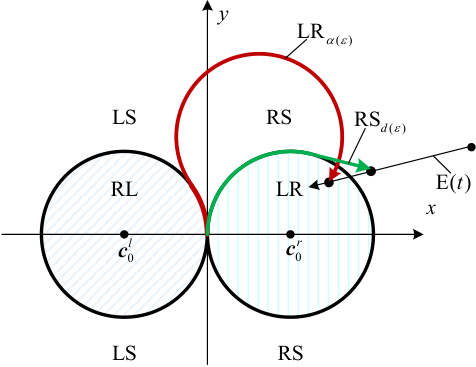
It is also known from [6] that for any sufficiently small we have , indicating that the function is discontinuous when the target moves from the circle into its inside. For the case that the target’s trajectory intersects the left half circle , it can be proven in the same way that the function is discontinuous at the intersection point.
From now on, we prove the necessity that the function is continuous if . Let us choose a time so that . According to [6, Section 3.3], given a sufficiently small , the path of RDP from to for any is of type RS. Thus, the function is continuous at if .
We choose a time so that . According to [6, Section 3.3], given a sufficiently small , the path of RDP from to for any keeps being of type LR. Thus, the function is continuous at if .
Then, we consider the rest case that there exists a time so that . Without loss of generality, let us assume that the target enters into the circle at . Then, there exists a small so that and . According to [6, Section 3.3], the paths of RDP from to , , and are of types RS, R, and LR. Note that if approaches to zero, the left turning circle and the straight line segment vanish. Thus, the function is continuous at if .
If the time is chosen so that , the continuity of can be proven in the same way, completing the proof.
Lemma 9
The minimum time for the pursuer to intercept the target is not smaller than , i.e., .
Proof of Lemma 9. According to the definitions of and , for any the value denotes the minimum time for the Dubins vehicle to move from to . Thus, the duration for the Dubins vehicle to move from to must be greater than , completing the proof.
Proof of Lemma 3. By contradiction, assume that the solution path of the MTIP does not follow that of the RDP from to . Notice that denotes the time for the Dubins vehicle to follow the solution path of RDP from to . Since the solution of RDP is the optimal path from to , the contradicting assumption implies . This contradicts the assumption of the lemma, completing the proof.
Proof of Theorem 1. (1) By contradiction, assume that is not a fixed point of . According to Lemma 9, this contradicting assumption implies . In view of Lemma 2, if , we have that is continuous around . Thus, there exists a sufficiently small so that
| (25) |
Since and is continuous, if is sufficiently small, it holds that . Then, according to [21, Theorem 2], for any there exists a feasible Dubins path with a duration of from initial condition to the point . For this reason, since by Eq. (25), it follows that there exists a feasible Dubins path with a duration of to reach the point . This means that the interception between the pursuer and the target can occur at a time , which is smaller than . By contraposition, the proof of the first statement is completed.
(2) Combining the first statement and Lemma 3, the second statement holds apparently.
Proof of Lemma 4. Given a path of type LuRv, the terminal point is expressed by [6]
According to this formula, if the terminal point continuously changes, the values of and continuously change as well. Thus, the functions and are continuous at , completing the proof.
Proof of Theorem 2. In view of the second statement of Lemma 5, for any given in the open interval, any feasible Dubins path with a duration of cannot start from and terminate at . Hence, in order to prove this theorem, we just need to prove that lies on the boundary of the interval .
By contradiction, assume . Note that and are continuous at according to Lemma 2 and Lemma 4, respectively. Hence, there exists a sufficiently small so that . According to the third statement of Lemma 5, for any in the interval , there exists a feasible Dubins path with a duration of from to the point . Thus, the target can be intercepted by the pursuer at the point by moving along a feasible Dubins path with a duration of , smaller than . By contraposition, we have that does not lie in the interior of the interval , i.e., .
From now on, we assume that lies in the open interval by contradiction. Note that is continuous at according to Lemma 4. Therefore, there exists a sufficiently small so that . Since , if is sufficiently small, it holds . Then, based on the third statement of Lemma 5, for any in the semi-open interval , there exists a feasible Dubins path from to the point with a duration of , smaller than . By contraposition, we have that does not lie in the open interval .
To sum up, it is concluded that lies on the boundary of , indicating that . Since is the minimum intercept time, we have that Eq. (14) holds, completing the proof.
Appendix B Proofs for the lemmas in Section 4
Proof of Lemma 6. This lemma is a direct result of the intermediate value theorem.
Proof of Lemma 7. Let be the radian of the right-turning circular arc R in the path of type RS, as presented in Fig. 14. By geometric analysis, we have
where is the length of the straight line segment and is the intercept point.

Because the pursuer and the target arrive at simultaneously, we have
| (34) |
Note that we have
indicating
| (35) |
Combining Eq. (34) and Eq. (35) yields
| (36) |
Substituting Eq. (35) and Eq. (36) into Eq. (B) to eliminate and , we have
| (37) |
where
Rearranging Eq. (37), we get
| (38) |
where
This concludes the proof of Lemma 7.
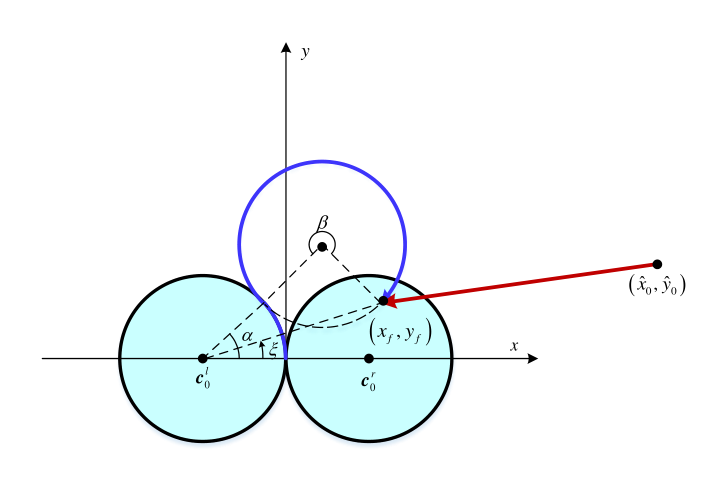
Note that
and
are located at the same point (the center of the circle coinciding with R). Thus, we have
As the pursuer and the target arrive at simultaneously, it follows that
| (45) |
We also have
| (46) |
Combining Eq. (45) with Eq. (46) leads to
| (47) | ||||
By the law of cosines, we also have
| (48) |
which leads to
| (49) |
Denote by the angle between -axis and the vector from to . Then, by using the law of sines, we have
| (50) |
where is the Euclidean distance between and the interception point . Taking into account the expression of , from Eq. (B) we get
| (51) |
Note that and . Then, according to Eq. (50), we have
| (52) |
Substituting Eq. (49) and Eq. (51) into Eq. (52), we can get
| (53) |
References
- [1] Rufus Isaacs. Differential Games: A Mathematical Theory with Applications to Warfare and Pursuit, Control and Optimization. Wiley, 1965.
- [2] Antony Willits Merz. The Homicidal Chauffeur: a Differential Game. Department of Aeronautics and Astronautics, Stanford University, 1971.
- [3] Alexey S. Matveev, Hamid Teimoori, and Andrey V. Savkin. Method for tracking of environmental level sets by a unicycle-like vehicle. Automatica, 48(9):2252 – 2261, 2012.
- [4] A. S. Matveev, H. Teimoori, and A. V. Savkin. A method for guidance and control of an autonomous vehicle in problems border patrolling and obstacle avoidance. Automatica, 47:515–524, 2011.
- [5] L. E. Dubins. On curves of minimal length with a constraint on average curvature, and with prescribed initial and terminal positions and tangents. American Journal of Mathematics, 79(3):497–516, 1957.
- [6] Jean-Daniel Boissonnat and Xuân-Nam Bui. Accessibility region for a car that only moves forwards along optimal paths. INRIA France, 1994.
- [7] H. J. Sussmann and G. Tang. Shortest paths for the reeds-shepp car: A worked out example of the use of geometric techniques in nonlinear optimal control. Technical report, Rutgers University, 1994.
- [8] L. S. Pontryagin, V. G. Boltyanski, R. V. Gamkrelidze, and E. F. Mishchenko. The Mathematical Theory of Optimal Processes (Russian). English translation: Interscience, 1962.
- [9] Zheng Chen and Tal Shima. Shortest Dubins paths through three points. Automatica, 105:368 – 375, 2019.
- [10] Yizhaq Meyer, Pantelis Isaiah, and Tal Shima. On dubins paths to intercept a moving target. Automatica, 53:256–263.
- [11] Akhil Gopalan, Ashwini Ratnoo, and Debasish Ghose. Time-optimal guidance for lateral interception of moving targets. Journal of Guidance, Control, and Dynamics, 39(3):510–525, 2016.
- [12] S. G. Manyam, D. Casbeer, A. Von Moll, and Z. Fuchs. Optimal dubins paths to intercept a moving target on a circle. In 2019 American Control Conference (ACC), pages 828–834, 2019.
- [13] Sanghyuk Park. Rendezvous guidance on circular path for fixed-wing uav. International Journal of Aeronautical and Space Sciences, pages 1–10, 2020.
- [14] Laszlo Techy and Craig A. Woolsey. Minimum-time path planning for unmanned aerial vehicles in steady uniform winds. Journal of Guidance, Control, and Dynamics, 32(6):1736–1746, November – December 2009.
- [15] Efstathios Bakolas and Panagiotis Tsiotras. Optimal synthesis of the zermelo-markov-dubins problem in a constant drift field. Journal of Optimization Theory and Applications, 156:469–492, 2013.
- [16] Timothy McGee and Karl Hedrick. Optimal path planning with a kinematic airplane model. Journal of Guidance, Control, and Dynamics, 30(2):629–633, 2007.
- [17] Timothy McGee, Stephen Spry, and Karl Hedrick. Optimal path planning in a constant wind with a bounded turning rate. In AIAA Guidance, Navigation, and Control Conference and Exhibit, pages 1–11, San Francisco, California, 2005.
- [18] Jason R. Looker. Minimum paths to interception of a moving target when constrained by turning radius. report DSTO-TR-2227, Air Operations Division, Defense Science and Technology Organisation, Austrilia, 2008.
- [19] Jean-Baptiste Caillau, S. Maslovskaya, T. Mensch, T. Moulinier, and J. Pomet. Zermelo-markov-dubins problem and extensions in marine navigation*. In 2019 IEEE 58th Conference on Decision and Control (CDC), pages 517–522, 2019.
- [20] Ernest Cockayne. Plane pursuit with curvature constraints. SIAM Journal on Applied Mathematics, 15(6):1511–1516, 1967.
- [21] Yulong Ding, Bin Xin, and Jie Chen. Curvature-constrained path elongation with expected length for dubins vehicle. Automatica, 108:1–8, 2019.