Neuroevolutionary learning of particles and protocols for self-assembly
Abstract
Within simulations of molecules deposited on a surface we show that neuroevolutionary learning can design particles and time-dependent protocols to promote self-assembly, without input from physical concepts such as thermal equilibrium or mechanical stability and without prior knowledge of candidate or competing structures. The learning algorithm is capable of both directed and exploratory design: it can assemble a material with a user-defined property, or search for novelty in the space of specified order parameters. In the latter mode it explores the space of what can be made rather than the space of structures that are low in energy but not necessarily kinetically accessible.
Introduction— How do we make a material with specified properties? In pursuit of “synthesis by design” De Yoreo et al. 2016; Broholm et al. 2016 the materials science community has developed and adapted algorithms of inverse design and machine learning. These approaches can identify interparticle potentials able to stabilize target structures or promote their self-assembly from solution Cohn and Kumar 2009; Torquato 2009; Bianchi et al. 2012; Rechtsman et al. 2006; Lindquist et al. 2016; Jadrich et al. 2017; Long and Ferguson 2018; Gadelrab et al. 2017; Ferguson 2017; Piñeros et al. 2018; van Anders et al. 2015; Adorf et al. 2018; Madge and Miller 2017; Jiang et al. 2018; Kumar et al. 2019; Zhou et al. 2019; Sherman et al. 2020; Reinhardt and Frenkel 2014; Romano et al. 2020; Miskin et al. 2016, and can identify protocols or reaction conditions that optimize the self-assembly of specified particles Klotsa and Jack 2013; Miskin et al. 2016; Raccuglia et al. 2016; Whitelam and Tamblyn 2020; Tang et al. 2016.
Here we present an approach based on evolutionary learning Holland 1992 that simultaneously designs particles and protocols in order to self-assemble materials to order. We study a coarse-grained computational model of molecular self-assembly at a surface Bartels 2010; Elemans et al. 2009; Swiegers and Malefetse 2002. Coarse-grained models are simple by design Doye et al. 2004; Hagan and Chandler 2006; Molinero and Moore 2008; Romano and Sciortino 2011; Glotzer et al. 2004; Doye et al. 2007; Rapaport 2010; Murugan et al. 2015; Whitelam and Jack 2015; Grunwald and Geissler 2014; Nguyen and Vaikuntanathan 2016; Lutsko 2019; Fan and Grunwald 2019; Carpenter and Grunwald 2020 but can exhibit key features of real systems, including the formation of complex structures and kinetic traps that impair assembly Thorkelsson et al. 2015; Biancaniello et al. 2005; Park et al. 2008; Nykypanchuk et al. 2008; Pfeifer and Saccà 2018; De Yoreo et al. 2015. The particular class of model we use here has been shown to reproduce the thermodynamic and dynamic behavior of a range of molecular and nanoscale assemblies at surfaces Whitelam et al. 2014. Such models provide a rigorous test of algorithmic control of self-assembly.
In order to allow thorough exploration of the self-assembly behavior accessible to this class of model we express the interparticle potential and time-dependent assembly protocol as arbitrary functions, encoded by neural networks. In evolutionary language, which reflects the method of learning used and provides a mnemonic for the role of each component of the algorithm, this encoding is the instruction code or “genome” for self-assembling a material. Molecular simulation carried out using the particle and protocols specified by the genome results in the “phenome”, a material whose properties can be measured and compared to a design goal.
Evolutionary learning on the parameters of the neural networks, called neuroevolution Holland 1992; Fogel and Stayton 1994; Salimans et al. 2017; Montana and Davis 1989; Such et al. 2017; Whitelam et al. 2020, can produce materials whose properties satisfy user-defined goals, which can be directed or exploratory in nature. The algorithm needs no information about possible candidate or competing structures, nor prior knowledge of what constitutes a good self-assembly protocol or particle design. For directed design we specify materials with certain pore geometries and isolated clusters of certain sizes. The solutions identified by the learning algorithm include interparticle interactions whose symmetries can be realized by known molecules or complexes Swiegers and Malefetse 2002; Bartels 2010; Elemans et al. 2009. The approach is simple to implement and can identify sophisticated design strategies, realizing complex structures via hierarchical self-assembly pathways. It can also fail, if the design goal is too challenging, and we discuss how to modify the goal in such cases.

Our approach is similar to that of Refs. Lindquist et al. 2016; Jadrich et al. 2017 in that we use an iterative learning method to promote self-assembly, but differs in that we do not specify or build the target structure in advance. In that respect it is similar to the approach of Ref. Miskin et al. 2016, and complementary to that work in that we express the design problem differently (in the form of neural networks) and optimize differently (via evolutionary methods). Our approach differs from other approaches to inverse design in that we consider the design of particles and protocols simultaneously, and do not appeal to physical concepts such as thermal equilibrium or mechanical stability. We also go beyond traditional forms of inverse design and borrow from the machine-learning literature to specify the design goal of novelty Conti et al. 2018. Within a space specified by certain order parameters we instruct the evolutionary learning algorithm to produce materials not seen previously, rather than materials with particular properties. If we specify materials with 3- and 4-membered pores then novelty search identifies structures dual to regular and semi-regular tilings of the plane and motifs that comprise 2D quasicrystals. In this mode the algorithm explores the space of what can be made rather than the space of structures that are low in energy but not necessarily kinetically accessible.
Model and learning algorithm— We consider a class of coarse-grained model able to capture the essential physics of molecular and nanoscale self-assembly at surfaces Whitelam et al. 2014. It comprises circular particles of hard-core diameter on a two-dimensional square substrate of side . The substrate has periodic boundary conditions in both directions. Particles evolve under a stochastic dynamical protocol consisting of a grand-canonical Monte Carlo algorithm with chemical potential , which allows particles to exchange with a notional solution Frenkel and Smit 1996, and the virtual-move Monte Carlo algorithm Whitelam et al. 2009; Hedges, which allows particles to move on the surface according to an approximation of Brownian motion Haxton et al. 2015. Grand-canonical moves are proposed with probability , where is the instantaneous number of particles on the surface Whitelam et al. 2014. All trajectories start from distinct disordered configurations consisting of 500 particles randomly deposited on the surface, and are run for Monte Carlo steps.
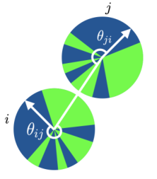
The angular component of the interparticle attraction and the time-dependent protocol are encoded as neural networks, specified in Section S1. Simulation potentials with angular dependence are often called “patchy” Zhang and Glotzer 2004. The interaction potential reflects the idea that particles interact in a complementary way, such as through DNA hybridization, hydrogen bonding, or other directional donor-acceptor mechanisms Swiegers and Malefetse 2002; Bartels 2010; Elemans et al. 2009; Pfeifer and Saccà 2016. The control parameters and influence the substrate density and the strength of interparticle attractions, which could be done in experiment by e.g. varying deposition rate and temperature (we call the process of increasing “cooling”). We denote the parameters of the neural networks by and . Using evolutionary language we call this encoding the material’s genome, an idea sketched in Fig. 1. The results of molecular simulation, using the potential and protocol defined by the genome, is the phenome.
To evolve genomes whose phenomes possess a desired property we use an iterative genetic algorithm consisting of a population dynamics combined with neuroevolution Holland 1992; Fogel and Stayton 1994; Salimans et al. 2017; Montana and Davis 1989; Such et al. 2017; Whitelam and Tamblyn 2020, specified in Section S2. Neuroevolution, stochastic mutation of the neural-network parameters, is equivalent in the limit of small mutations to gradient descent in the presence of Gaussian white noise Whitelam et al. 2020. The learning algorithm starts in Generation 0 with a population of 100 randomly-chosen genomes, and “expresses” their phenomes via steps of the molecular simulation protocol described above. The algorithm identifies the 10 phenomes possessing the largest values of an objective function . The 10 corresponding genomes are cloned and mutated in order to produce a new population (or generation) of 100 genomes, whose phenomes are then expressed via molecular simulation. This iterative procedure continues, generation by generation, until terminated by the user.
The objective function or evolutionary pressure is a user-specified order parameter , evaluated at the final time point of each simulation. In this work we consider order parameters built from two quantities. One is , the number of clusters of interacting particles of size (called -mers). The other is , the number of convex loops of size (called -gons) that can be drawn by joining the centers of interacting particles. -gons are pores: designing materials with specified pore sizes is useful for e.g. gas separation Liu et al. 2016.


Directed search— We direct the algorithm to evolve a material containing convex pores of size 12, and set . This case provides an example of an objective that is too complex to achieve without additional guidance: 12-gons are sufficiently complex that they do not form spontaneously under the random particle- and protocol design that comprises the initial stage (Generation 0) of the learning algorithm. All phenomes score zero, and the learning algorithm has nothing to work with. In this case a simple modification of the objective is sufficient to overcome the problem. We set , where is the size of the largest convex pore seen across all 100 phenomes of a given generation. Thus if is 12 or larger then the learning algorithm selects genomes that produce 12-gons; if is smaller than 12 then it selects genomes that produce -gons.
The results of several generations of learning using this objective are shown in Fig. 2. The largest pore sizes seen in the first 4 generations are 10, 9, 11, and 11, and thereafter the first 12-gons are produced. The learning algorithm improves its design and the yield of 12-gons over evolutionary time, and eventually achieves the self-assembly of a structure dual to the 3.12.12 Archimedean tiling, which has one 3-gon and two 12-gons around each vertex Grunbaum and Shephard 1977; Antlanger et al. 2011; Whitelam 2016. To do so requires a sophisticated design. The particle must present sticky patches whose bisectors are separated (approximately) by angles and . In addition, the patches must be inequivalent: if all patches possess equal binding energy then kinetic traps impair the formation of the structure Whitelam 2016. The solution identified by the learning algorithm is to make one patch weaker than the other two, and to steadily cool the substrate. The result is a hierarchical dynamics that starts with many isolated 3-gons forming from the engagement of the strong patches. Eventually the weak patches engage and cause the 3-gons to form a network, which subsequently forms 12-gons [Fig. S2]. The learning algorithm also evacuates the substrate, removing steric impediments to closure of the network. The resulting strategy produces a yield of 12-gons superior to that achieved by a human-designed particle and protocol [Fig. S3(a)].
In Fig. 3 we show the results of evolutionary learning instructed to make 4-mers, 5-mers and 5-gons, and 6-gons. In each case the strategy learned is efficient: to produce 4-mers the algorithm evolves particles with two patches separated by an angle , leading to compact square clusters; to make pentagonal 5-gons it evolves particles with patches separated by an angle ; and to make 6-gons the algorithm evolves particles with approximate 3-fold rotational symmetry, which self-assemble under the learned protocol into the honeycomb lattice. Similar motifs are seen in a range of real system that realize the honeycomb lattice Swiegers and Malefetse 2002; Bartels 2010; Elemans et al. 2009; Whitelam et al. 2014. The evolutionary pressure to achieve geometrical perfection of the interaction is relatively weak: self-assembly of a particle with perfect three-fold rotational symmetry and a learned time-dependent protocol results in a comparable yield of 6-gons [Fig. S3(b)]. The evolutionary trajectories showing the emergence of these designs are shown in Figs. S4, S5, and S6.

Exploratory search— We end by showing that evolutionary learning can be used in an exploratory mode, searching for novelty rather than to achieve a desired property Conti et al. 2018. To search for novelty within the space of 4-gons and 3-gons we impose the objective function
| (1) |
where runs over all phenomes produced in all previous and current generations. Maximizing (1) leads to an evolutionary pressure favoring materials most unlike those produced to date, rather than materials with specified values of and . Over the course of 10 generations of novelty search the learning algorithm produces the coverage of space shown in Fig. 4. Some of the polygon structures dual to the particle structures found during that exploration are shown in the figure. These include size-limited motifs; the square and triangle regular tilings of the plane; the 3.6.3.6 and 3.3.3.4.4 Archimedean tilings Grunbaum and Shephard 1977; Antlanger et al. 2011; Whitelam 2016; and the , H, and Z binding motifs prominent in dodecagonal quasicrystals van der Linden et al. 2012. The particle that gives rise to those motifs is shown in the figure: it has irregular six-fold symmetry, different to the five-fold and seven-fold coordination known to form similar motifs van der Linden et al. 2012. A larger section of the material made by this particle is shown in Fig. S7.
Conclusions— We have shown that a neuroevolutionary learning algorithm can identify particles and protocols for the self-assembly of materials with desired properties, without input from physical principles and with no prior knowledge of self-assembly. The learning algorithm is capable of both directed and exploratory design. It can assemble a material with a user-defined property, or search for novelty in the space of specified order parameters. In the latter mode it explores the space of what can be made rather than the space of structures that are low in energy but not necessarily kinetically accessible. Moreover, the approach described here can be used to address design problems of considerable complexity: the neural-network encoding of potential and protocol extends to an arbitrary number of inputs and outputs, and evolutionary learning works with large numbers of parameters Such et al. 2017; Salimans et al. 2017.
Acknowledgments – This work was performed as part of a user project at the Molecular Foundry, Lawrence Berkeley National Laboratory, supported by the Office of Science, Office of Basic Energy Sciences, of the U.S. Department of Energy under Contract No. DE-AC02–05CH11231. I.T. acknowledges NSERC and performed work at the NRC under the auspices of the AI4D and MCF Programs.
References
- De Yoreo et al. (2016) J. De Yoreo, D. Mandrus, L. Soderholm, T. Forbes, M. Kanatzidis, J. Erlebacher, J. Laskin, U. Wiesner, T. Xu, S. Billinge, et al., Basic Research Needs Workshop on Synthesis Science for Energy Relevant Technology, Tech. Rep. (USDOE Office of Science (SC)(United States), 2016).
- Broholm et al. (2016) C. Broholm, I. Fisher, J. Moore, M. Murnane, A. Moreo, J. Tranquada, D. Basov, J. Freericks, M. Aronson, A. MacDonald, et al., Basic Research Needs Workshop on Quantum Materials for Energy Relevant Technology, Tech. Rep. (USDOE Office of Science (SC)(United States), 2016).
- Cohn and Kumar (2009) H. Cohn and A. Kumar, Proceedings of the National Academy of Sciences 106, 9570 (2009).
- Torquato (2009) S. Torquato, Soft Matter 5, 1157 (2009).
- Bianchi et al. (2012) E. Bianchi, G. Doppelbauer, L. Filion, M. Dijkstra, and G. Kahl, The Journal of Chemical Physics 136, 214102 (2012).
- Rechtsman et al. (2006) M. C. Rechtsman, F. H. Stillinger, and S. Torquato, Physical Review E 74, 021404 (2006).
- Lindquist et al. (2016) B. A. Lindquist, R. B. Jadrich, and T. M. Truskett, Journal of Chemical Physics 145 (2016).
- Jadrich et al. (2017) R. Jadrich, B. Lindquist, and T. Truskett, The Journal of Chemical Physics 146, 184103 (2017).
- Long and Ferguson (2018) A. W. Long and A. L. Ferguson, Molecular Systems Design & Engineering 3, 49 (2018).
- Gadelrab et al. (2017) K. R. Gadelrab, A. F. Hannon, C. A. Ross, and A. Alexander-Katz, Molecular Systems Design & Engineering 2, 539 (2017).
- Ferguson (2017) A. L. Ferguson, Journal of Physics: Condensed Matter 30, 043002 (2017).
- Piñeros et al. (2018) W. D. Piñeros, B. A. Lindquist, R. B. Jadrich, and T. M. Truskett, The Journal of Chemical Physics 148, 104509 (2018).
- van Anders et al. (2015) G. van Anders, D. Klotsa, A. S. Karas, P. M. Dodd, and S. C. Glotzer, ACS Nano 9, 9542 (2015).
- Adorf et al. (2018) C. S. Adorf, J. Antonaglia, J. Dshemuchadse, and S. C. Glotzer, The Journal of Chemical Physics 149, 204102 (2018).
- Madge and Miller (2017) J. Madge and M. A. Miller, Soft matter 13, 7780 (2017).
- Jiang et al. (2018) X. Jiang, J. Li, V. Lee, H. M. Jaeger, O. G. Heinonen, and J. J. de Pablo, The Journal of Chemical Physics 148, 234302 (2018).
- Kumar et al. (2019) R. Kumar, G. M. Coli, M. Dijkstra, and S. Sastry, The Journal of Chemical Physics 151, 084109 (2019).
- Zhou et al. (2019) P. Zhou, J. C. Proctor, G. van Anders, and S. C. Glotzer, Molecular Physics 117, 3968 (2019).
- Sherman et al. (2020) Z. M. Sherman, M. P. Howard, B. A. Lindquist, R. B. Jadrich, and T. M. Truskett, The Journal of Chemical Physics 152, 140902 (2020).
- Reinhardt and Frenkel (2014) A. Reinhardt and D. Frenkel, Physical Review Letters 112, 238103 (2014).
- Romano et al. (2020) F. Romano, J. Russo, L. Kroc, and P. Šulc, Physical Review Letters 125, 118003 (2020).
- Miskin et al. (2016) M. Z. Miskin, G. Khaira, J. J. de Pablo, and H. M. Jaeger, Proceedings of the National Academy of Sciences 113, 34 (2016).
- Klotsa and Jack (2013) D. Klotsa and R. L. Jack, The Journal of Chemical Physics 138, 094502 (2013).
- Raccuglia et al. (2016) P. Raccuglia, K. C. Elbert, P. D. Adler, C. Falk, M. B. Wenny, A. Mollo, M. Zeller, S. A. Friedler, J. Schrier, and A. J. Norquist, Nature 533, 73 (2016).
- Whitelam and Tamblyn (2020) S. Whitelam and I. Tamblyn, Physical Review E 101, 052604 (2020).
- Tang et al. (2016) X. Tang, B. Rupp, Y. Yang, T. D. Edwards, M. A. Grover, and M. A. Bevan, ACS Nano 10, 6791 (2016).
- Holland (1992) J. H. Holland, Scientific american 267, 66 (1992).
- Bartels (2010) L. Bartels, Nature Chemistry 2, 87 (2010).
- Elemans et al. (2009) J. A. A. W. Elemans, S. Lei, and S. De Feyter, Angewandte Chemie International Edition 48, 7298 (2009).
- Swiegers and Malefetse (2002) G. F. Swiegers and T. J. Malefetse, Coordination chemistry reviews 225, 91 (2002).
- Doye et al. (2004) J. P. K. Doye, A. A. Louis, and M. Vendruscolo, Physical Biology 1, P9 (2004).
- Hagan and Chandler (2006) M. F. Hagan and D. Chandler, Biophysical Journal 91, 42 (2006).
- Molinero and Moore (2008) V. Molinero and E. B. Moore, The Journal of Physical Chemistry B 113, 4008 (2008).
- Romano and Sciortino (2011) F. Romano and F. Sciortino, Nature materials 10, 171 (2011).
- Glotzer et al. (2004) S. Glotzer, M. Solomon, and N. A. Kotov, AIChE Journal 50, 2978 (2004).
- Doye et al. (2007) J. P. K. Doye, A. A. Louis, I. C. Lin, L. R. Allen, E. G. Noya, A. W. Wilber, H. C. Kok, and R. Lyus, Physical Chemistry Chemical Physics 9, 2197 (2007).
- Rapaport (2010) D. C. Rapaport, Phys. Biol. 7, 045001 (2010).
- Murugan et al. (2015) A. Murugan, J. Zou, and M. P. Brenner, Nature Communications 6 (2015).
- Whitelam and Jack (2015) S. Whitelam and R. L. Jack, Annual Review of Physical Chemistry 66, 143 (2015).
- Grunwald and Geissler (2014) M. Grunwald and P. L. Geissler, ACS Nano 8, 5891 (2014).
- Nguyen and Vaikuntanathan (2016) M. Nguyen and S. Vaikuntanathan, Proceedings of the National Academy of Sciences 113, 14231 (2016).
- Lutsko (2019) J. F. Lutsko, Science advances 5, eaav7399 (2019).
- Fan and Grunwald (2019) Z. Fan and M. Grunwald, Journal of the American Chemical Society 141, 1980 (2019).
- Carpenter and Grunwald (2020) J. E. Carpenter and M. Grunwald, Journal of the American Chemical Society 142, 10755 (2020).
- Thorkelsson et al. (2015) K. Thorkelsson, P. Bai, and T. Xu, Nano Today 10, 48 (2015).
- Biancaniello et al. (2005) P. L. Biancaniello, A. J. Kim, and J. C. Crocker, Physical Review Letters 94, 058302 (2005).
- Park et al. (2008) S. Y. Park, A. K. Lytton-Jean, B. Lee, S. Weigand, G. C. Schatz, and C. A. Mirkin, Nature 451, 553 (2008).
- Nykypanchuk et al. (2008) D. Nykypanchuk, M. M. Maye, D. van der Lelie, and O. Gang, Nature 451, 549 (2008).
- Pfeifer and Saccà (2018) W. Pfeifer and B. Saccà, Biological Chemistry 399, 773 (2018).
- De Yoreo et al. (2015) J. J. De Yoreo, P. U. Gilbert, N. A. Sommerdijk, R. L. Penn, S. Whitelam, D. Joester, H. Zhang, J. D. Rimer, A. Navrotsky, J. F. Banfield, et al., Science 349, aaa6760 (2015).
- Whitelam et al. (2014) S. Whitelam, I. Tamblyn, T. K. Haxton, M. B. Wieland, N. R. Champness, J. P. Garrahan, and P. H. Beton, Physical Review X 4, 011044 (2014).
- Fogel and Stayton (1994) D. B. Fogel and L. C. Stayton, BioSystems 32, 171 (1994).
- Salimans et al. (2017) T. Salimans, J. Ho, X. Chen, S. Sidor, and I. Sutskever, arXiv preprint arXiv:1703.03864 (2017).
- Montana and Davis (1989) D. J. Montana and L. Davis, in IJCAI, Vol. 89 (1989) pp. 762–767.
- Such et al. (2017) F. P. Such, V. Madhavan, E. Conti, J. Lehman, K. O. Stanley, and J. Clune, arXiv preprint arXiv:1712.06567 (2017).
- Whitelam et al. (2020) S. Whitelam, V. Selin, S.-W. Park, and I. Tamblyn, arXiv preprint arXiv:2008.06643 (2020).
- Conti et al. (2018) E. Conti, V. Madhavan, F. P. Such, J. Lehman, K. Stanley, and J. Clune, in Advances in neural information processing systems (2018) pp. 5027–5038.
- Frenkel and Smit (1996) D. Frenkel and B. Smit, Understanding Molecular Simulation: From Algorithms to Applications (Academic Press, Inc. Orlando, FL, USA, 1996).
- Whitelam et al. (2009) S. Whitelam, E. H. Feng, M. F. Hagan, and P. L. Geissler, Soft Matter 5, 1251 (2009).
- (60) L. O. Hedges, “http://vmmc.xyz,” .
- Haxton et al. (2015) T. K. Haxton, L. O. Hedges, and S. Whitelam, Soft matter 11, 9307 (2015).
- Zhang and Glotzer (2004) Z. Zhang and S. C. Glotzer, Nano Letters 4, 1407 (2004).
- Pfeifer and Saccà (2016) W. Pfeifer and B. Saccà, ChemBioChem 17, 1063 (2016).
- Liu et al. (2016) G. Liu, W. Jin, and N. Xu, Angewandte Chemie International Edition 55, 13384 (2016).
- Grunbaum and Shephard (1977) B. Grunbaum and G. C. Shephard, Mathematics Magazine 50, 227 (1977).
- Antlanger et al. (2011) M. Antlanger, G. Doppelbauer, and G. Kahl, Journal of Physics: Condensed Matter 23, 404206 (2011).
- Whitelam (2016) S. Whitelam, Physical Review Letters 117, 228003 (2016).
- van der Linden et al. (2012) M. N. van der Linden, J. P. Doye, and A. A. Louis, The Journal of Chemical Physics 136, 054904 (2012).
S1 Neural-network encoding of potential and protocol
Interparticle attraction and time-dependent assembly protocols are encoded as single-layer neural networks of hidden nodes, sketched in Fig. 1. Particles possess an attractive interaction of range . The angular component of the interaction is the radial-basis-function neural network
| (S1) |
containing trainable parameters . If lies outside the interval then it is set to the appropriate edge of the interval. In images, angular portions of the particle corresponding to are colored green, and are otherwise blue. Initially (in Generation 0) we set , , and choose the to be Gaussian random numbers. The potential remains fixed for all time within each simulation. For computational efficiency we evaluate the neural network only once, at the start of the simulation, in order to create a lookup table for with discretized over 1000 points on the interval .
Two particles and whose centers are a distance apart, where , experience an energy of interaction
| (S2) |
Here sets the scale of the interaction. is the angle (in an anti-clockwise sense) between two lines, the line joining the center of particle to the point specified by on its circumference, and the line joining the center of particle to the center of particle : see Fig. S1. The minimum function encodes the idea that particles interact in a complementary way, such as through DNA hybridization, hydrogen bonding, or other directional donor-acceptor mechanisms.
The time-dependent protocol is encoded by a second neural network. Each trajectory starts with control-parameter values and . 1000 times within each trajectory, at time increments of , the control parameters are set to the new values and , where the neural network
| (S3) | |||||
contains trainable parameters . If moves outwith the interval it is returned to the appropriate edge of the interval. Initially (in Generation 0) all parameters of this network are Gaussian random numbers, .
S2 Evolutionary learning algorithm
The evolutionary algorithm starts with 100 molecular simulations using distinct genomes , randomized as described in Section S1. This set of 100 simulations is called Generation 0, and, following molecular simulation, results in 100 phenomes. Let quantify the design goal (e.g. the number of clusters or pores of a certain size). The algorithm selects the 10 genomes responsible for the phenomes having the 10 largest values of , choosing randomly in the event of equal scores. (For the novelty search used to produce Fig. 4 we selected the top 25 phenomes, rather than the top 10). To create the 100 genomes that comprise Generation 1 it draws 100 times randomly with replacement from this set of 10 genomes, and mutates each by a set of Gaussian random numbers,
| (S4) |
Here with , and with . The parameters and are chosen independently for each simulation, as the absolute value of the Gaussian random numbers and , respectively. Doing so results in a combination of many small mutations and the occasional large mutation. Molecular simulation of this new set of 100 genomes results in the 100 phenomes of Generation 1, and so on.
S3 Supplementary figures


