跳到论文正文
W Papers独立论文阅读器 arXiv:2012.11822 论文正文 计算阅读时间 · 0%
引用这篇论文根据当前论文元数据生成,正式投稿前建议核对。


License: CC BY 4.0
arXiv:2012.11822v2 [cond-mat.stat-mech] 01 Sep 2021

Supplementary Information for “Exceptional Dynamical Quantum Phase Transitions in Periodically Driven Systems”

Ryusuke Hamazaki Affiliation: Nonequilibrium Quantum Statistical Mechanics RIKEN Hakubi Research Team, RIKEN Cluster for Pioneering Research (CPR), RIKEN iTHEMS, Wako, Saitama 351-0198, Japan

Supplementary Note 1: Dynamical phase transitions for other parameters and initial/final states

Here, we describe in detail dynamical phases and their transitions of the stroboscopic Ising model for situations different from that presented in the main text. Supplementary Figure 1 shows examples of dynamical quantum phase transitions (DQPTs) of F∞,TTrF_{\mathrm{\infty,T}}^{\mathrm{Tr}} for T=7T=7 and T=8T=8 with J=0.25​πJ=0.25\pi with varying bb. As discussed in the main text and Supplementary Note 6, neffn_{\mathrm{eff}} [the number of degenerate eigenvalues with the largest modulus of U~\tilde{U}] is always equal to or larger than 2 for T=7T=7 because the system belongs to Class AII (neff≥4n_{\mathrm{eff}}\geq 4 comes from additional symmetry U~\tilde{U}, such as the translation invariance). Therefore no exceptional DQPT occurs in this case. On the other hand, we find the exceptional DQPT for T=8T=8, indicating that the exceptional DQPT is the general mechanism that can occur in systems with Class AI-type antiunitary symmetry.

Next, Supplementary Figure 2 shows the case where we vary parameters other than bb. We find that the exceptional DQPT can occur for J=0.25​πJ=0.25\pi even when hh is varied for fixed appropriate bb, which indicates the divergence of the generalized observable ⟨σ1z⟩gexp\braket{\sigma_{1}^{z}}_{\mathrm{gexp}}. On the other hand, the exceptional DQPT does not occur if JJ is varied since antiunitary symmetry no longer exists in U~\tilde{U}.

Finally, Supplementary Figure 3 shows the bb-dependence of F∞,T↑⁣↑F_{\infty,T}^{\uparrow\uparrow} and F∞,T↓⁣↑F_{\infty,T}^{\downarrow\uparrow} for J=0.25​πJ=0.25\pi and T=7T=7. As detailed in Supplementary Note 3, U~↓⁣↑\tilde{U}_{\mathrm{\downarrow\uparrow}} has Class AI antiunitary symmetry for odd TT, but U~↑⁣↑\tilde{U}_{\mathrm{\uparrow\uparrow}} does not. Thus, while we can find the exceptional DQPT for F∞,T↓⁣↑F_{\infty,T}^{\downarrow\uparrow} but not for F∞,T↑⁣↑F_{\infty,T}^{\uparrow\uparrow}.

Refer to caption
Figure 1: Supplementary Figure 1. (Real part of) dynamical free energy F∞,TTrF^{\mathrm{Tr}}_{\infty,T} as a function of bb for different transient times TT. As varying bb, the exceptional dynamical quantum phase transition (DQPT) occurs for T=8T=8, which is prohibited for T=7T=7. Purple numbers denote ndegn_{\mathrm{deg}} for each phase. We use h=0.5h=0.5 and J=0.25​πJ=0.25\pi.
Refer to caption
Figure 2: Supplementary Figure 2. (Real part of) dynamical free energy F∞,TTrF^{\mathrm{Tr}}_{\infty,T} as a function of hh and JJ. As a function of hh, we have several exceptional dynamical quantum phase transitions (DQPTs), where J=0.25​πJ=0.25\pi, b=0.05​πb=0.05\pi and T=6T=6 are used. On the other hand, no exceptional DQPT exists as a function of JJ because of the absence of the hidden antiunitary symmetry of U~\tilde{U} (h=3h=3, b=−0.25​πb=-0.25\pi and T=6T=6 are used).
Refer to caption
Figure 3: Supplementary Figure 3. (Real part of) dynamical free energy F∞,T↑⁣↑F^{\uparrow\uparrow}_{\infty,T} and F∞,T↓⁣↑F^{\downarrow\uparrow}_{\infty,T} as a function of bb. The exceptional dynamical quantum phase transition (DQPT) occurs only for F∞,T↓⁣↑F^{\downarrow\uparrow}_{\infty,T}. Note that ndegn_{\mathrm{deg}} changes from 2 to 1 at the exceptional DQPT as increasing bb. We use h=2,J=−0.25​πh=2,J=-0.25\pi and T=7T=7 for both of the data.

Supplementary Note 2: Derivation of spacetime-dual operators

Here, we describe in detail the derivation of the spacetime-dual operators to calculate the dynamical free energies, following Refs. [1, 2, 3]. We first seek for the representation for U~Tr\tilde{U}_{\mathrm{Tr}}, which satisfies

Tr⁡[UT]2L=Tr⁡[U~TrL]\displaystyle\frac{\mathrm{Tr}[U^{T}]}{2^{L}}=\mathrm{Tr}[\tilde{U}_{\mathrm{Tr}}^{L}] (1)

or equivalently

FL,TTr=−log⁡|Tr⁡[U~TrL]|L.\displaystyle F^{\mathrm{Tr}}_{L,T}=-\frac{\log|\mathrm{Tr}[\tilde{U}_{\mathrm{Tr}}^{L}]|}{L}. (2)

For this purpose, we notice

Tr⁡[UT]\displaystyle\mathrm{Tr}[U^{T}] =∑{𝐬τ}∏τ=1T⟨𝐬τ+1|e−i∑j=1Lbσjxe−i∑j=1LJσjzσj+1z−i∑j=1Lhσjz|𝐬τ⟩\displaystyle=\sum_{\left\{\mathbf{s}_{\tau}\right\}}\prod_{\tau=1}^{T}\braket{\mathbf{s}_{\tau+1}|e^{-i\sum_{j=1}^{L}b\sigma_{j}^{x}}e^{-i\sum_{j=1}^{L}J\sigma_{j}^{z}\sigma_{j+1}^{z}-i\sum_{j=1}^{L}h\sigma_{j}^{z}}|\mathbf{s}_{\tau}}
=(sin⁡2​b2​i)L​T/2∑{sτ,j}e−i∑τ=1T∑j=1L(Jsτ,jsτ,j+1+J′sτ,jsτ+1,j+hsτ,j),\displaystyle=\left(\frac{\sin 2b}{2i}\right)^{LT/2}\sum_{\left\{s_{\tau,j}\right\}}e^{-i\sum_{\tau=1}^{T}\sum_{j=1}^{L}(Js_{\tau,j}s_{\tau,j+1}+J^{\prime}s_{\tau,j}s_{\tau+1,j}+hs_{\tau,j})}, (3)

where |𝐬τ⟩\ket{\mathbf{s}_{\tau}} are the computational basis, sτ,js_{\tau,j} are classical spin variables taking ±1\pm 1, and J′=−π4−i2​log⁡tan⁡bJ^{\prime}=-\frac{\pi}{4}-\frac{i}{2}\log\tan b. On the other hand, we can consider

U~′Tr=e−i∑τ=1Tb~σxτe−i∑τ=1T(J~σzτσzτ+1+hστz),\displaystyle\tilde{U}^{\prime}_{\mathrm{Tr}}=e^{-i\sum_{\tau=1}^{T}\tilde{b}\sigma^{x}_{\tau}}e^{-i\sum_{\tau=1}^{T}(\tilde{J}\sigma^{z}_{\tau}\sigma^{z}_{\tau+1}+{h}\sigma_{\tau}^{z})}, (4)

which satisfies

Tr[U~Tr′L]=(sin⁡2​b~2​i)L​T/2∑{sτ,j}e−i∑τ=1T∑j=1L(J~′sτ,jsτ,j+1+J~sτ,jsτ+1,j+hsτ,j)\displaystyle\mathrm{Tr}[\tilde{U}^{\prime L}_{\mathrm{Tr}}]=\left(\frac{\sin 2\tilde{b}}{2i}\right)^{LT/2}\sum_{\left\{s_{\tau,j}\right\}}e^{-i\sum_{\tau=1}^{T}\sum_{j=1}^{L}(\tilde{J}^{\prime}s_{\tau,j}s_{\tau,j+1}+\tilde{J}s_{\tau,j}s_{\tau+1,j}+hs_{\tau,j})} (5)

with J~′=−π4−i2​log⁡tan⁡b~\tilde{J}^{\prime}=-\frac{\pi}{4}-\frac{i}{2}\log\tan\tilde{b}. Then, introducing a normalization constant

C=12​(sin⁡2​bsin⁡2​b~)L​T2\displaystyle C=\frac{1}{2}\left(\frac{\sin 2b}{\sin 2\tilde{b}}\right)^{\frac{LT}{2}} (6)

and setting b~=arctan⁡[e2​i​(J+π/4)]=i2​log⁡(1+e2​i​J1−e2​i​J)=−π4−i2​log⁡tan⁡J\tilde{b}=\mathrm{arctan}[e^{2i(J+\pi/4)}]=\frac{i}{2}\log\left(\frac{1+e^{2iJ}}{1-e^{2iJ}}\right)=-\frac{\pi}{4}-\frac{i}{2}\log\tan J (to satisfy J~′=J\tilde{J}^{\prime}=J) with J~=J′\tilde{J}=J^{\prime}, we have

U~Tr=CU~′Tr=Ce−i∑τ=1Tb~σxτe−i∑τ=1T(J~σzτσzτ+1+hστz),\displaystyle\tilde{U}_{\mathrm{Tr}}=C\tilde{U}^{\prime}_{\mathrm{Tr}}=Ce^{-i\sum_{\tau=1}^{T}\tilde{b}\sigma^{x}_{\tau}}e^{-i\sum_{\tau=1}^{T}(\tilde{J}\sigma^{z}_{\tau}\sigma^{z}_{\tau+1}+{h}\sigma_{\tau}^{z})}, (7)

which satisfies Supplementary Equation (1) as desired.

Next, U~↑↑/↓↑\tilde{U}_{\uparrow\uparrow/\downarrow\uparrow} can be calculated similarly. We show that they are represented as

U~↑↑/↓↑=C′e−i∑τ=1T−1b~στxe−i∑τ=1T−2J~στzστ+1z−i∑τ=1T−1hστz−iJ~(σ1z+IσT−1z)\displaystyle\tilde{U}_{\uparrow\uparrow/\downarrow\uparrow}=C^{\prime}e^{-i\sum_{\tau=1}^{T-1}\tilde{b}\sigma_{\tau}^{x}}e^{-i\sum_{\tau=1}^{T-2}\tilde{J}\sigma_{\tau}^{z}\sigma_{\tau+1}^{z}-i\sum_{\tau=1}^{T-1}h\sigma_{\tau}^{z}-i\tilde{J}(\sigma_{1}^{z}+I\sigma_{T-1}^{z})} (8)

with the open boundary condition, where C′=(sin⁡2​b/2​i)1/2​(sin⁡2​b/sin⁡2​b~)(T−1)/2​e−i⁡(h+J)C^{\prime}=(\sin 2b/2i)^{1/2}(\sin 2b/\sin 2\tilde{b})^{(T-1)/2}e^{-i(h+J)} , and I=1​(−1)I=1\>(-1) for U~↑⁣↑​(U~↓⁣↑)\tilde{U}_{\uparrow\uparrow}\>(\tilde{U}_{\downarrow\uparrow}). To see this, we notice (for |ψf⟩=|↑⋯↑⟩/|↓⋯↓⟩\ket{\psi_{f}}=\ket{\uparrow\cdots\uparrow}/\ket{\downarrow\cdots\downarrow})

⟨ψf|UT|↑⋯↑⟩=\displaystyle\braket{\psi_{f}|U^{T}|\uparrow\cdots\uparrow}= ∑{𝐬τ}⟨ψf|U|𝐬T−1⟩⋯⟨𝐬1|U|↑⋯↑⟩\displaystyle\sum_{{\left\{\mathbf{s}_{\tau}\right\}}}\braket{\psi_{f}|U|\mathbf{s}_{T-1}}\cdots\braket{\mathbf{s}_{1}|U|\uparrow\cdots\uparrow}
=(sin⁡2​b2​i)L​T/2∑{sτ,j}\displaystyle=\left(\frac{\sin 2b}{2i}\right)^{LT/2}\sum_{{\left\{s_{\tau,j}\right\}}} e−i∑τ=1T−1∑j=1LJsτ,jsτ,j+1+hsτ,j−i∑τ=1T−2∑j=1LJ′sτ,jsτ+1,j\displaystyle e^{-i\sum_{\tau=1}^{T-1}\sum_{j=1}^{L}Js_{\tau,j}s_{\tau,j+1}+hs_{\tau,j}-i\sum_{\tau=1}^{T-2}\sum_{j=1}^{L}J^{\prime}s_{\tau,j}s_{\tau+1,j}}
×e−i∑j=1L{(J+h)+J′s1,j+J′IsT−1,j},\displaystyle\times e^{-i\sum_{j=1}^{L}{\left\{(J+h)+J^{\prime}s_{1,j}+J^{\prime}Is_{T-1,j}\right\}}}, (9)

where I=1I=1 for |ψf⟩=|↑⋯↑⟩\ket{\psi_{f}}=\ket{\uparrow\cdots\uparrow} and I=−1I=-1 for |ψf⟩=|↓⋯↓⟩\ket{\psi_{f}}=\ket{\downarrow\cdots\downarrow}. To construct dual operators, we consider (T−1)(T-1)-spins along time with the open boundary condition. In fact, if we assume Supplementary Equation (8), we find

F↑↑/↓↑L,T=−log|Tr[U~↑↑/↓↑L]|L.\displaystyle F^{\uparrow\uparrow/\downarrow\uparrow}_{L,T}=-\frac{\log|\mathrm{Tr}[\tilde{U}_{\uparrow\uparrow/\downarrow\uparrow}^{L}]|}{L}. (10)

Supplementary Note 3: Existence of antiunitary symmetry

Here, we describe in detail the antiunitary symmetry (AUS) of the spacetime-dual operator. First, we show that the spacetime-dual operator U~Tr\tilde{U}_{\mathrm{Tr}} with J=π4+n​π2​(n∈ℤ)J=\frac{\pi}{4}+\frac{n\pi}{2}\>(n\in\mathbb{Z}) satisfies

V​U~Tr∗​V†=ei​ϕ​U~Tr,\displaystyle V\tilde{U}_{\mathrm{Tr}}^{*}V^{\dagger}=e^{i\phi}\tilde{U}_{\mathrm{Tr}}, (11)

where

V=∏τ=1Tei​π2​στy\displaystyle V=\prod_{\tau=1}^{T}e^{i\frac{\pi}{2}\sigma_{\tau}^{y}} (12)

and ϕ∈ℝ\phi\in\mathbb{R}.

For J=π4+n​π2​(n∈ℤ)J=\frac{\pi}{4}+\frac{n\pi}{2}\>(n\in\mathbb{Z}), b~=±π/4\tilde{b}=\pm\pi/4 becomes real. Noticing J~=−π4−i2​log⁡tan⁡b=−J~∗−π2\tilde{J}=-\frac{\pi}{4}-\frac{i}{2}\log\tan b=-\tilde{J}^{*}-\frac{\pi}{2}, the left-hand side of Supplementary Equation (11) becomes

V​U~Tr∗​V†\displaystyle V\tilde{U}_{\mathrm{Tr}}^{*}V^{\dagger} =C​V​ei​∑τ=1Tb~​στx​V†​V​ei​∑τ=1T(J~∗​στz​στ+1z+h​στz)​V†\displaystyle=CVe^{i\sum_{\tau=1}^{T}\tilde{b}\sigma^{x}_{\tau}}V^{\dagger}Ve^{i\sum_{\tau=1}^{T}(\tilde{J}^{*}\sigma^{z}_{\tau}\sigma^{z}_{\tau+1}+{h}\sigma_{\tau}^{z})}V^{\dagger}
=e−i∑τ=1Tb~σxτei​∑τ=1T(J~∗​στz​στ+1z−h​στz)\displaystyle=e^{-i\sum_{\tau=1}^{T}\tilde{b}\sigma^{x}_{\tau}}e^{i\sum_{\tau=1}^{T}(\tilde{J}^{*}\sigma^{z}_{\tau}\sigma^{z}_{\tau+1}-{h}\sigma_{\tau}^{z})}
=e−i∑τ=1Tb~σxτe−i∑τ=1T(J~σzτσzτ+1+hστz)e−iπ2∑τ=1Tσzτσzτ+1\displaystyle=e^{-i\sum_{\tau=1}^{T}\tilde{b}\sigma^{x}_{\tau}}e^{-i\sum_{\tau=1}^{T}(\tilde{J}\sigma^{z}_{\tau}\sigma^{z}_{\tau+1}+{h}\sigma_{\tau}^{z})}e^{-i\frac{\pi}{2}\sum_{\tau=1}^{T}\sigma^{z}_{\tau}\sigma^{z}_{\tau+1}}
=U~Tr​∏τ=1T(−i​στz​στ+1z)=(−i)T​U~Tr,\displaystyle=\tilde{U}_{\mathrm{Tr}}\prod_{\tau=1}^{T}\left(-i\sigma_{\tau}^{z}\sigma_{\tau+1}^{z}\right)=(-i)^{T}\tilde{U}_{\mathrm{Tr}}, (13)

which is the right-hand side. Since V​V∗=𝕀VV^{*}=\mathbb{I} for even TT and −𝕀-\mathbb{I} for odd TT, U~Tr\tilde{U}_{\mathrm{Tr}} belongs to Class AI for even TT and Class AII for odd TT.

Next, we show that U~↓⁣↑\tilde{U}_{\downarrow\uparrow} with J=π4+n​π2​(n∈ℤ)J=\frac{\pi}{4}+\frac{n\pi}{2}\>(n\in\mathbb{Z}) satisfies

V​U~↓⁣↑∗​V†=ei​ϕ​U~↓⁣↑,\displaystyle V\tilde{U}_{\downarrow\uparrow}^{*}V^{\dagger}=e^{i\phi}\tilde{U}_{\downarrow\uparrow}, (14)

where

V=𝒫​∏τ=1T−1ei​π2​στy\displaystyle V=\mathcal{P}\prod_{\tau=1}^{T-1}e^{i\frac{\pi}{2}\sigma_{\tau}^{y}} (15)

and ϕ∈ℝ\phi\in\mathbb{R}. Here, 𝒫\mathcal{P} is the parity operator exchanging the site τ\tau and T−τT-\tau. In fact, the left-hand side of Supplementary Equation (14) becomes

V​U~↓⁣↑∗​V†\displaystyle V\tilde{U}_{\downarrow\uparrow}^{*}V^{\dagger} =C′⁣∗​V​ei​∑τ=1T−1b~​στx​V†​V​ei​∑τ=1T−2J~∗​στz​στ+1z+i​∑τ=1T−1h​στz+i​J~∗​(σ1z−σT−1z)​V†\displaystyle=C^{\prime*}Ve^{i\sum_{\tau=1}^{T-1}\tilde{b}\sigma_{\tau}^{x}}V^{\dagger}Ve^{i\sum_{\tau=1}^{T-2}\tilde{J}^{*}\sigma_{\tau}^{z}\sigma_{\tau+1}^{z}+i\sum_{\tau=1}^{T-1}h\sigma_{\tau}^{z}+i\tilde{J}^{*}(\sigma_{1}^{z}-\sigma_{T-1}^{z})}V^{\dagger}
=ei​ζC′e−i∑τ=1T−1b~στxei​∑τ=1T−2J~∗​στz​στ+1z−i​∑τ=1T−1h​στz−i​J~∗​(−σ1z+σT−1z)\displaystyle=e^{i\zeta}C^{\prime}e^{-i\sum_{\tau=1}^{T-1}\tilde{b}\sigma_{\tau}^{x}}e^{i\sum_{\tau=1}^{T-2}\tilde{J}^{*}\sigma_{\tau}^{z}\sigma_{\tau+1}^{z}-i\sum_{\tau=1}^{T-1}h\sigma_{\tau}^{z}-i\tilde{J}^{*}(-\sigma_{1}^{z}+\sigma_{T-1}^{z})}
=ei​ζU~↓⁣↑e−iπ2∑τ=1T−1στzστ+1z+iπ2(−σ1z+σT−1z)\displaystyle=e^{i\zeta}\tilde{U}_{\downarrow\uparrow}e^{-i\frac{\pi}{2}\sum_{\tau=1}^{T-1}\sigma_{\tau}^{z}\sigma_{\tau+1}^{z}+i\frac{\pi}{2}(-\sigma_{1}^{z}+\sigma_{T-1}^{z})}
=ei​ζ​U~↓⁣↑​σ1z​σT−1z​∏τ=1T−1(−i​στz​στ+1z)\displaystyle=e^{i\zeta}\tilde{U}_{\downarrow\uparrow}\sigma_{1}^{z}\sigma_{T-1}^{z}\prod_{\tau=1}^{T-1}\left(-i\sigma_{\tau}^{z}\sigma_{\tau+1}^{z}\right)
=ei​ζ​(−i)T−1​U~↓⁣↑,\displaystyle=e^{i\zeta}(-i)^{T-1}\tilde{U}_{\downarrow\uparrow}, (16)

which is the right-hand side. Here, we have used b~∈ℝ\tilde{b}\in\mathbb{R} for J=π4+n​π2​(n∈ℤ)J=\frac{\pi}{4}+\frac{n\pi}{2}\>(n\in\mathbb{Z}), J~∗=−(J~+π/2)\tilde{J}^{*}=-(\tilde{J}+\pi/2), C′⁣∗/C′=ei​ζ​(ζ∈ℝ)C^{\prime*}/C^{\prime}=e^{i\zeta}\>(\zeta\in\mathbb{R}), and 𝒫​σ1​𝒫=σT−1\mathcal{P}\sigma_{1}\mathcal{P}=\sigma_{T-1}. Since V​V∗=𝕀VV^{*}=\mathbb{I} for odd TT and −𝕀-\mathbb{I} for even TT, U~↓⁣↑\tilde{U}_{\downarrow\uparrow} belongs to Class AI for odd TT and Class AII for even TT.

We note that the minus sign associated with the exchange between σ1z−σT−1z\sigma_{1}^{z}-\sigma_{T-1}^{z} under parity operation is essential for this antiunitary symmetry. This is not possible for U~↑⁣↑\tilde{U}_{\uparrow\uparrow}, where σ1z+σT−1z\sigma_{1}^{z}+\sigma_{T-1}^{z} is invariant under the parity operation.

Supplementary Note 4: Thermalization of the expectation values of local observables averaged over a long time

As mentioned in the main text, DQPTs in our model do not appear as an infinite-time average of expectation values of local observables because of the Floquet eigenstate thermalization hypothesis [4]. To demonstrate this, here we numerically show that the time-averaged expectation values of local observables become the thermalized values.

We particularly consider a time-averaged expectation value of local magnetization

mz¯=1T​∑t=1T⟨ψi|U−t​σi=1z​Ut|ψi⟩,\displaystyle\overline{m^{z}}=\frac{1}{T}\sum_{t=1}^{T}\braket{\psi_{i}|U^{-t}\sigma_{i=1}^{z}U^{t}|\psi_{i}}, (17)

and that of local correlation

Cz​z¯=1T​∑t=1T⟨ψi|U−t​σi=1z​σi=2z​Ut|ψi⟩,\displaystyle\overline{C^{zz}}=\frac{1}{T}\sum_{t=1}^{T}\braket{\psi_{i}|U^{-t}\sigma_{i=1}^{z}\sigma_{i=2}^{z}U^{t}|\psi_{i}}, (18)

where TT is sufficiently large. If the system thermalizes, mz¯\overline{m^{z}} and Cz​z¯\overline{C^{zz}} will be equal to the expectation value at the infinite temperature, i.e., Tr⁡[σi=1z]/2L=Tr⁡[σi=1z​σi=2z]/2L=0\mathrm{Tr}[\sigma_{i=1}^{z}]/2^{L}=\mathrm{Tr}[\sigma_{i=1}^{z}\sigma_{i=2}^{z}]/2^{L}=0. In the following, we take an initial state as |ψi⟩=|↑↑⋯↑⟩\ket{\psi_{i}}=\ket{\uparrow\uparrow\cdots\uparrow}. We remind that the DQPTs (including the exceptional DQPT) occur for several bb for F∞,T{↑↑/↓↑}F_{\infty,T}^{{\left\{\uparrow\uparrow/\downarrow\uparrow\right\}}} with finite TT starting from this initial state (see Supplementary Note 1).

Supplementary Figure 4 shows the values of mz¯\overline{m^{z}} and Cz​z¯\overline{C^{zz}} as a function of bb for different system sizes LL. We find that mz¯\overline{m^{z}} and Cz​z¯\overline{C^{zz}} approach zero as increasing the system size especially for bb far from the integrable point (b/π=0,0.5,1b/\pi=0,0.5,1), which indicates that they become zero in the thermodynamic limit. This implies that our DQPTs are unique to finite-time regimes, in which time serves as an important parameter in stark contrast with conventional phase transitions.

Refer to caption
Figure 4: Supplementary Figure 4. Long time average of the expectation values of local observables in a. Supplementary Equation (17) and b. Supplementary Equation (18) as a function of bb. We show results for different system sizes, L=8L=8 (blue), 10 (black) 12 (yellow), 14 (red), and 16 (green). We find that mz¯\overline{m^{z}} and Cz​z¯\overline{C^{zz}} approach zero as increasing the system size especially for bb far from the integrable point (b/π=0,0.5,1b/\pi=0,0.5,1), which indicates that they become zero in the thermodynamic limit. This means that, while we have several dynamical quantum phase transitions of F∞,T{↑↑/↓↑}F_{\infty,T}^{{\left\{\uparrow\uparrow/\downarrow\uparrow\right\}}} with finite TT for the displayed range of bb, long-time-averages of the expectation values thermalize to the values described by the infinite-temperature state. We use T=1000T=1000, J=−0,25​πJ=-0,25\pi and h=1.3​πh=1.3\pi.

Supplementary Note 5: Dynamical phase transition at the self-dual point

In this section, we discuss the details for the DQPT occurring at the self-dual points, i.e., J=π4+n​π2J=\frac{\pi}{4}+\frac{n\pi}{2} and b=π4+m​π2​(n,m∈ℤ)b=\frac{\pi}{4}+\frac{m\pi}{2}\>(n,m\in\mathbb{Z}) [2, 3]. We especially show that crossing self-dual points entails DQPTs universally for FTr/↑↑/↓↑∞,TF^{\mathrm{Tr}/\uparrow\uparrow/\downarrow\uparrow}_{\infty,T} with any TT and hh, whose singularity is analogous to that for the conventional DQPT. Moreover, the dynamical free energy density takes a universal value as F∞,TTr=log⁡2F^{\mathrm{Tr}}_{\infty,T}=\log 2 or F↑↑/↓↑∞,T=log2/2F^{\uparrow\uparrow/\downarrow\uparrow}_{\infty,T}=\log 2/2 there.

We especially focus on the case for FTrF_{\mathrm{Tr}} (other dynamical free energies are discussed in a similar manner). As discussed in the main text, we can exactly write

U~Tr=Ce−i∑τ=1Tb~στxe−i∑τ=1TJ~στzστ+1z−i∑τ=1Thστz\displaystyle\tilde{U}_{\mathrm{Tr}}=Ce^{-i\sum_{\tau=1}^{T}\tilde{b}\sigma_{\tau}^{x}}e^{-i\sum_{\tau=1}^{T}\tilde{J}\sigma_{\tau}^{z}\sigma_{\tau+1}^{z}-i\sum_{\tau=1}^{T}h\sigma_{\tau}^{z}} (19)

using the spacetime duality [1, 2, 3]. Here, b~=−π/4−ilog(tanJ)/2\tilde{b}=-\pi/4-i\log(\tan J)/2, J~=−π/4−ilog(tanb)/2\tilde{J}=-\pi/4-i\log(\tan b)/2 and C=(sin⁡2​b/sin⁡2​b~)T/2/2C=(\sin 2b/\sin 2\tilde{b})^{T/2}/2. Importantly, U~\tilde{U} is unitary (up to a constant) only at the self-dual points.

As noted in the main text, for typical cases, DQPTs occur when maximum of two eigenvalues with different θα\theta_{\alpha} switches accidentally, where ndeg=1n_{\mathrm{deg}}=1 for each phase and ndeg=2n_{\mathrm{deg}}=2 at transition (Supplementary Figure 5a). On the other hand, DQPT occurs more universally if the self-dual point is crossed: all of the modulus of the eigenvalues of U~\tilde{U} are equal at this point (ndeg=2Tn_{\mathrm{deg}}=2^{T}), and crossing this point typically switches the largest eigenvalue (Supplementary Figure 5b). At transition, dynamical free energies are determined only by the modulus of the eigenvalues, which leads to universal values F∞,TTr=log⁡2F^{\mathrm{Tr}}_{\infty,T}=\log 2 (similarly, we have F↑↑/↓↑∞,T=log2/2F^{\uparrow\uparrow/\downarrow\uparrow}_{\infty,T}=\log 2/2). To our best knowledge, this is the first evidence that the self-dual point is a critical point of different dynamical phases.

Refer to caption
Figure 5: Supplementary Figure 5. Schematic of eigenvalue dynamics of the spacetime-dual operator U~\tilde{U} and its relation to the dynamical quantum phase transition (DQPT). a. Typical eigenvalue dynamics (small circles) near DQPT. Green dashed circles have the radius that corresponds to the eigenvalue(s) with the largest modulus. The eigenvalue with the largest modulus (red circles) switches at the critical point, at which two eigenvalues have the same modulus ndeg=2n_{\mathrm{deg}}=2. b. Eigenvalue dynamics through the DQPT induced by self-dual points. At the self-dual point, all of 2T2^{T} numbers of eigenvalues have the same modulus owing to the unitarity of U~\tilde{U}.

Supplementary Note 6: Dynamical phase transitions in finite systems

Here, we show several results concerning the DQPTs for finite system size LL.

Degeneracy and finite-size effect

While the number of eigenvalues with maximum modulus ndegn_{\mathrm{deg}} does not contribute to the free energy density for L→∞L\rightarrow\infty, ndegn_{\mathrm{deg}} can characterize each phase via a finite-size correction Δ​FL,T=FL,T−F∞,T\Delta F_{L,T}=F_{L,T}-F_{\infty,T}. Indeed, the second term in

FL,T≃−log⁡|λM|−1L​log⁡|∑αei​θα​L|.\displaystyle F_{L,T}\simeq-\log|\lambda_{\mathrm{M}}|-\frac{1}{L}\log\left|\sum_{\alpha}e^{i\theta_{\alpha}L}\right|. (20)

shows that Δ​FL,T\Delta F_{L,T} is upper bounded by log⁡ndeg/L\log n_{\mathrm{deg}}/L, where the bound is achieved when ei​θα​L=ei​θβ​Le^{i\theta_{\alpha}L}=e^{i\theta_{\beta}L} for every α≠β\alpha\neq\beta.

Supplementary Figure 6a shows the finite-size scaling of Δ​FL,TTr\Delta F_{L,T}^{\mathrm{Tr}} near the exceptional DQPT. While Δ​FL,TTr\Delta F_{L,T}^{\mathrm{Tr}} exponentially decays with LL for b<bcb<b_{c} since ndeg=1n_{\mathrm{deg}}=1, it exhibits polynomially decaying oscillations for b>bcb>b_{c}, where the decay is upper bounded by log⁡ndeg/L=log⁡2/L\log n_{\mathrm{deg}}/L=\log 2/L for sufficiently large LL. At the transition point, oscillation-free polynomial decay is observed. Another example is the behavior at the self-dual point, where the decay is upper bounded by log⁡2T/L\log 2^{T}/L (Supplementary Figure 6b).

Refer to caption
Figure 6: Supplementary Figure 6. Log-log plot for finite-size correction of the dynamical free energy density Δ​FL,TTr\Delta F_{L,T}^{\mathrm{Tr}}. a. Behavior near the exceptional dynamical quantum phase transition (DQPT). Below the DQPT with ndeg=1n_{\mathrm{deg}}=1 (blue), Δ​FL,TTr\Delta F_{L,T}^{\mathrm{Tr}} decays rapidly. (inset) Semi-log plot of the same data shows that it indeed decays exponentially (dotted red line is an eyeguide for exponential decay). Above the DQPT with ndeg=2n_{\mathrm{deg}}=2 (green), Δ​FL,TTr\Delta F_{L,T}^{\mathrm{Tr}} decays with oscillations. The decay is bounded by log⁡2/L\log 2/L (red solid line) for sufficiently large LL. Approaching the critical point (black), the oscillation vanishes and Δ​FL,TTr∼log⁡2/L\Delta F_{L,T}^{\mathrm{Tr}}\sim\log 2/L. b. Behavior at the self-dual point (purple), where ndeg=2T=64n_{\mathrm{deg}}=2^{T}=64. The correction is bounded by log⁡64/L\log 64/L. We use J=−π/4J=-\pi/4 and h=3.0h=3.0, and T=6T=6.

The number ndegn_{\mathrm{deg}} thus provides universal information through Δ​FL,T\Delta F_{L,T} on dynamical phases, which is deeply related to the symmetries hidden in the space-time dual operator U~\tilde{U}. If U~\tilde{U} is in Class AI (FL,TTrF^{\mathrm{Tr}}_{L,T} with even TT and FL,T↓⁣↑F^{\downarrow\uparrow}_{L,T} with odd TT under the condition J=−π/4+nπ/2(n∈ℤ)J=-\pi/4+n\pi/2\>(n\in\mathbb{Z})), phases with ndeg=2n_{\mathrm{deg}}=2 can naturally appear as well as phases with ndeg=1n_{\mathrm{deg}}=1. If U~\tilde{U} is in Class AII (FL,TTrF^{\mathrm{Tr}}_{L,T} with odd TT and FL,T↓⁣↑F^{\downarrow\uparrow}_{L,T} with even TT under the condition J=−π/4+nπ/2(n∈ℤ)J=-\pi/4+n\pi/2\>(n\in\mathbb{Z})), all phases satisfy ndeg≥2n_{\mathrm{deg}}\geq 2. We note that other symmetries are found to exist that enhance the value of ndegn_{\mathrm{deg}}, such as translation invariance for U~Tr\tilde{U}_{\mathrm{Tr}} or integrability at h=0h=0, which may also be interesting to study systematically.

Generalized correlation function in small systems

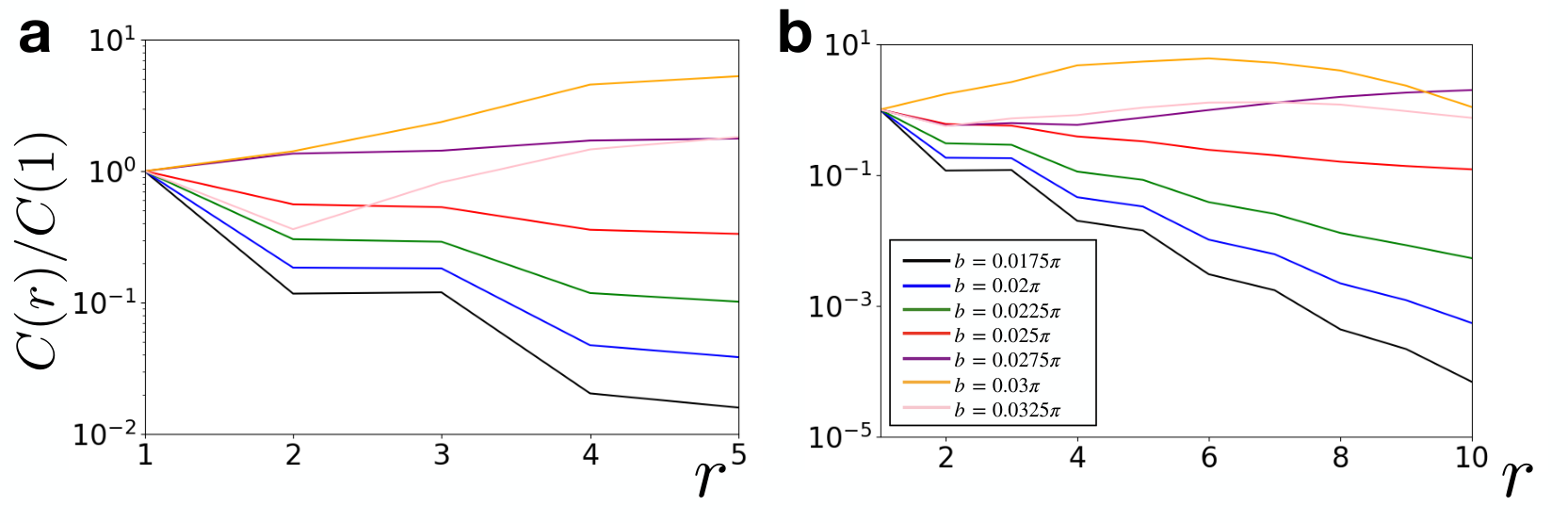
While the true DQPT occurs in the thermodynamic limit, qualitative signature of AUS-unbroken and AUS-broken phases are already captured even for finite system sizes with the generalized correlation function. In Supplementary Figure 7, we show the (normalized) generalized correlation function for different system size LL. Even for L=10L=10, which has been prepared in experiments of trapped ions [5], we find clear difference between AUS-unbroken (b<bc≃0.0257​πb<b_{c}\simeq 0.0257\pi) and AUS-broken (b>bcb>b_{c}) regime. Indeed, C⁡(r)C(r) decays fast for the former but does not decay for the latter. If we consider L=20L=20, we can also see the oscillatory behavior in the AUS-broken regime: note that the oscillation length is evaluated as ξosc≃10.4\xi_{\mathrm{osc}}\simeq 10.4 for b=0.03​πb=0.03\pi and ξosc≃8.5\xi_{\mathrm{osc}}\simeq 8.5 for b=0.0325​πb=0.0325\pi.

Refer to caption
Figure 7: Supplementary Figure 7. Normalized generalized correlation function C⁡(r)/C⁡(0)C(r)/C(0) for different values of bb. a. Results for L=10L=10. Clear difference between antiunitary-symmetry (AUS) unbroken (b<bc≃0.0257​πb<b_{c}\simeq 0.0257\pi) and AUS broken (b>bcb>b_{c}) regimes already appears. Indeed, C⁡(r)C(r) decays fast for the former but does not decay for the latter. b. Results for L=20L=20. The oscillatory behavior in the AUS-broken regime arises, where the oscillation length is evaluated as ξosc≃10.4\xi_{\mathrm{osc}}\simeq 10.4 for b=0.03​πb=0.03\pi and ξosc≃8.5\xi_{\mathrm{osc}}\simeq 8.5 for b=0.0325​πb=0.0325\pi. We use J=−π/4J=-\pi/4 and h=3.0h=3.0, and T=6T=6.

Supplementary Note 7: Explicit construction of an order parameter

We here show that we can explicitly construct an order parameter using different-time generalized observables. For this purpose, we especially focus on FL,T↓⁣↑=−1L​log⁡|⟨ψf|UT|ψi⟩|F^{\downarrow\uparrow}_{L,T}=-\frac{1}{L}\log|\braket{\psi_{f}|U^{T}|\psi_{i}}| with |ψi⟩=|↑⋯↑⟩\ket{\psi_{i}}=\ket{\uparrow\cdots\uparrow} and |ψf⟩=|↓⋯↓⟩\ket{\psi_{f}}=\ket{\downarrow\cdots\downarrow}, instead of FL,TTrF^{\mathrm{Tr}}_{L,T}, since its operational meaning in experimental situations is more direct. We note that F∞,T↓⁣↑F^{\downarrow\uparrow}_{\infty,T} shows the exceptional DQPT for b=bc≃0.446​πb=b_{c}\simeq 0.446\pi with h=1.3h=1.3, T=5T=5 and J=−π/4J=-\pi/4, where the AUS is broken for b<bcb<b_{c} and unbroken for b>bcb>b_{c} (note that this is opposite to the case for F∞,TTrF^{\mathrm{Tr}}_{\infty,T}).

For our discussion, we first note that, for a usual symmetry breaking, such as ℤ2\mathbb{Z}_{2} symmetry breaking of an Ising model, magnetization mzm^{z} becomes an order parameter. In this case, mzm^{z} is odd under symmetry operation (mz→−mzm^{z}\rightarrow-m^{z}), so ⟨mz⟩=−⟨mz⟩=0\braket{m^{z}}=-\braket{m^{z}}=0 when symmetry of the state is unbroken.

Similarly, our antiunitary symmetry operation in the space-time dual space (V=𝒫​∏τ=1T−1ei​π2​στyV=\mathcal{P}\prod_{\tau=1}^{T-1}e^{i\frac{\pi}{2}\sigma_{\tau}^{y}} for U~↓⁣↑\tilde{U}_{\downarrow\uparrow}) is found to correspond to a combined symmetry of time exchange τ↔T−τ\tau\leftrightarrow T-\tau, complex conjugation, and certain spin reversal in the original space. For example, using the spacetime-dual transformation and the spectral decomposition U~↓⁣↑=∑αλα​|ϕα⟩​⟨χα|\tilde{U}_{\downarrow\uparrow}=\sum_{\alpha}\lambda_{\alpha}\ket{\phi_{\alpha}}\bra{\chi_{\alpha}}, we have

⟨ψf|UT−τ​σiz​Uτ|ψi⟩\displaystyle\braket{\psi_{f}|U^{T-\tau}\sigma_{i}^{z}U^{\tau}|\psi_{i}} =Tr⁡[U~↓⁣↑L​στz]\displaystyle=\mathrm{Tr}[\tilde{U}_{\downarrow\uparrow}^{L}\sigma_{\tau}^{z}] (21)
→λ0L​⟨χ0|στz|ϕ0⟩\displaystyle\rightarrow\lambda_{0}^{L}\braket{\chi_{0}|\sigma_{\tau}^{z}|\phi_{0}} (22)

for the symmetry-unbroken phase, where 0 labels the eigenvalues with the largest modulus. In this phase, we have

V​|ϕ0⟩∗=|ϕ0⟩,V​|χ0⟩∗=|χ0⟩,\displaystyle V\ket{\phi_{0}}^{*}=\ket{\phi_{0}},\quad V\ket{\chi_{0}}^{*}=\ket{\chi_{0}}, (23)

and thus

⟨χ0|στz|ϕ0⟩\displaystyle\braket{\chi_{0}|\sigma_{\tau}^{z}|\phi_{0}} =⟨χ0∗|V†​στz​V|ϕ0∗⟩=−⟨χ0|σT−τz|ϕ0⟩∗\displaystyle=\braket{\chi_{0}^{*}|V^{\dagger}\sigma_{\tau}^{z}V|\phi_{0}^{*}}=-\braket{\chi_{0}|\sigma_{T-\tau}^{z}|\phi_{0}}^{*} (24)

Then, we find that Re⁡[⟨ψf|UT−τ​σiz​Uτ|ψi⟩]=−Re⁡[⟨ψf|Uτ​σiz​UT−τ|ψi⟩]\mathrm{Re}[\braket{\psi_{f}|U^{T-\tau}\sigma_{i}^{z}U^{\tau}|\psi_{i}}]=-\mathrm{Re}[\braket{\psi_{f}|U^{\tau}\sigma_{i}^{z}U^{T-\tau}|\psi_{i}}] if the symmetry is unbroken [the spin indices ii is arbitrary]. On the other hand, we can also find Re⁡[⟨ψf|UT−τ​σiz​Uτ|ψi⟩]≠−Re⁡[⟨ψf|Uτ​σiz​UT−τ|ψi⟩]\mathrm{Re}[\braket{\psi_{f}|U^{T-\tau}\sigma_{i}^{z}U^{\tau}|\psi_{i}}]\neq-\mathrm{Re}[\braket{\psi_{f}|U^{\tau}\sigma_{i}^{z}U^{T-\tau}|\psi_{i}}] for the symmetry-breaking phase.

Refer to caption
Figure 8: Supplementary Figure 8. The order parameter in Supplementary Equation (25). a, Schematic illustration of the behavior for MM for infinite system size. b, Numerical verification. The exceptional dynamical quantum phase transition for FL,T↓⁣↑F^{\downarrow\uparrow}_{L,T} occurs for b=bc≃0.446​πb=b_{c}\simeq 0.446\pi, where b<bcb<b_{c} represents the symmetry-broken and b>bcb>b_{c} represents the symmetry-unbroken phase. We find M≠0M\neq 0 for b<bcb<b_{c} and M≃0M\simeq 0 for b>bcb>b_{c} (the deviation from zero and the finite peak are due to the finite symmetry-breaking term, which is required for finite LL). We use L=800L=800, T=5T=5, J=−0.2498​πJ=-0.2498\pi and h=1.3h=1.3.

Then, we can explicitly construct the following order parameter using generalized observables:

M=|Re⁡[∑τ=1T−1⟨ψf|UT−τ​σiz​Uτ|ψi⟩⟨ψf|UT|ψi⟩]|2.\displaystyle M=\left|\mathrm{Re}\left[\sum_{\tau=1}^{T-1}\frac{\braket{\psi_{f}|U^{T-\tau}\sigma_{i}^{z}U^{\tau}|\psi_{i}}}{\braket{\psi_{f}|U^{T}|\psi_{i}}}\right]\right|^{2}. (25)

When the antiunitary symmetry is unbroken, M=0M=0, and when it is broken, M≠0M\neq 0 and behaves as ∼|b−bc|−1\sim|b-b_{c}|^{-1} at criticality (Supplementary Figure 8a). As shown in Supplementary Figure 8b, we can demonstrate this using a numerical simulation. Here, the slight deviation from M=0M=0 for the symmetry-unbroken phase and the finite peak at the critical point are due to the finite symmetry-breaking term, which is required for finite LL to demonstrate the symmetry breaking.

We note that MM is constructed using the different-time generalized observables rather than a single-time expectation value of local observables. In the above example, MM diagnoses symmetry of interference structure in quantum dynamics related to the time-reversal operation τ↔T−τ\tau\leftrightarrow T-\tau.

Supplementary Note 8: Other models that exhibit exceptional DQPT

Floquet unitary circuits

Here, we describe in detail that exceptional DQPT can occur in certain Floquet unitary circuits, in addition to our stroboscopic Ising model. We assume that the system size LL is even and consider the unitary circuit given in the form as

U=∏j:even𝒰j,j+1∏j:odd𝒰j,j+1,\displaystyle U=\prod_{j\mathrm{:even}}\mathcal{U}_{j,j+1}\prod_{j\mathrm{:odd}}\mathcal{U}_{j,j+1}, (26)

which is composed of two-site unitary circuits 𝒰j,j+1\mathcal{U}_{j,j+1} (Supplementary Figure 9). When the dimension of the local Hilbert space is two (i.e., spin-1/2 systems), such two-site unitary circuits can be generally represented as [6]

𝒰j,j+1=ei​ξ​(uj⊗uj+1)​𝒱​(vj⊗vj+1),\displaystyle\mathcal{U}_{j,j+1}=e^{i\xi}(u_{j}\otimes u_{j+1})\mathcal{V}(v_{j}\otimes v_{j+1}), (27)

where uju_{j} and vjv_{j} are one-site unitary operators, ξ∈ℝ\xi\in\mathbb{R}, and 𝒱\mathcal{V} can be parametrized as

𝒱=e−i⁡(J1​σjx​σj+1x+J2​σjy​σj+1y+J3​σjz​σj+1z)\displaystyle\mathcal{V}=e^{-i(J_{1}\sigma^{x}_{j}\sigma^{x}_{j+1}+J_{2}\sigma^{y}_{j}\sigma^{y}_{j+1}+J_{3}\sigma^{z}_{j}\sigma^{z}_{j+1})} (28)

using J1,J2,J3∈ℝJ_{1},J_{2},J_{3}\in\mathbb{R}. For simplicity, we assume that uj=uu_{j}=u and vj=vv_{j}=v are jj-independent in the following.

We now focus on time evolution for T/2T/2 steps, which correspond to the total time T(∈2​ℕ)T\>(\in 2\mathbb{N}), and the following (real part of) dynamical free energy:

FL,T/2Tr=−1L​log⁡|Tr⁡[UT/2]|+log⁡2.\displaystyle F^{\mathrm{Tr}}_{L,T/2}=-\frac{1}{L}\log|\mathrm{Tr}[U^{T/2}]|+\log 2. (29)

We require that the spacetime-dual operator U~\tilde{U} of UU should satisfy

FL,T/2Tr=−1L​log⁡|Tr⁡[U~L/2]|,\displaystyle F^{\mathrm{Tr}}_{L,T/2}=-\frac{1}{L}\log|\mathrm{Tr}[\tilde{U}^{L/2}]|, (30)

with which F∞,T/2TrF^{\mathrm{Tr}}_{\infty,T/2} is given by −(log|λM|)/2-(\log|\lambda_{\mathrm{M}}|)/2.

By considering the dual operators for 𝒰j,j+1\mathcal{U}_{j,j+1} [6], we find

U~=14∏τ:even𝒰~τ,τ+1∏τ:odd𝒰~τ,τ+1,\displaystyle\tilde{U}=\frac{1}{4}\prod_{\tau\mathrm{:even}}\tilde{\mathcal{U}}_{\tau,\tau+1}\prod_{\tau\mathrm{:odd}}\mathcal{\tilde{U}}_{\tau,\tau+1}, (31)

where

𝒰~τ,τ+1=ei​ξ​(vT⊗u)​𝒱~τ,τ+1​(v⊗uT).\displaystyle\tilde{\mathcal{U}}_{\tau,\tau+1}=e^{i\xi}(v^{\mathrm{T}}\otimes u)\tilde{\mathcal{V}}_{\tau,\tau+1}(v\otimes u^{\mathrm{T}}). (32)

Here,

𝒱~τ,τ+1=12​e−i​J3+i​J−​στz​στ+1z+12​e−i​J3−i​J−+12​ei​J3−i​J+​στx​στ+1x−12​ei​J3+i​J+​στy​στ+1y\displaystyle\tilde{\mathcal{V}}_{\tau,\tau+1}=\frac{1}{2}e^{-iJ_{3}+iJ_{-}}\sigma^{z}_{\tau}\sigma^{z}_{\tau+1}+\frac{1}{2}e^{-iJ_{3}-iJ_{-}}+\frac{1}{2}e^{iJ_{3}-iJ_{+}}\sigma^{x}_{\tau}\sigma^{x}_{\tau+1}-\frac{1}{2}e^{iJ_{3}+iJ_{+}}\sigma^{y}_{\tau}\sigma^{y}_{\tau+1} (33)

with J±=J1±J2J_{\pm}=J_{1}\pm J_{2} and vTv^{\mathrm{T}} denotes the transposition of vv. It can also be written as [6]

[e−i​J3​cos⁡(J−)00ei​J3​cos⁡(J+)0−i​e−i​J3​sin⁡(J−)−i​ei​J3​sin⁡(J+)00−i​ei​J3​sin⁡(J+)−i​e−i​J3​sin⁡(J−)0ei​J3​cos⁡(J+)00e−i​J3​cos⁡(J−)].\displaystyle\left[\begin{array}[]{cccc}e^{-iJ_{3}}\cos\left(J_{-}\right)&0&0&e^{iJ_{3}}\cos\left(J_{+}\right)\\ 0&-ie^{-iJ_{3}}\sin\left(J_{-}\right)&-ie^{iJ_{3}}\sin\left(J_{+}\right)&0\\ 0&-ie^{iJ_{3}}\sin\left(J_{+}\right)&-ie^{-iJ_{3}}\sin\left(J_{-}\right)&0\\ e^{iJ_{3}}\cos\left(J_{+}\right)&0&0&e^{-iJ_{3}}\cos\left(J_{-}\right)\end{array}\right].
Figure 9: Supplementary Figure 9. Schematic illustration of the Floquet circuit dynamics in Supplementary Equation (26). We show the example for L=12L=12 and T=6T=6. Each of the block 𝒰j,j+1\mathcal{U}_{j,j+1} can be written as in Supplementary Equation (27).

Antiunitary symmetry

To discuss the existence of the exceptional DQPT, we restrict ourselves to ξ=0\xi=0 and

u=v=e−i​h2​σz,\displaystyle u=v=e^{-i\frac{h}{2}\sigma^{z}}, (38)

which correspond to the presence of the uniform magnetic field. To simplify the notation, we consider the unitary transformation for U~→(u⊗u)​U~​(u†⊗u†)\tilde{U}\rightarrow(u\otimes u)\tilde{U}(u^{\dagger}\otimes u^{\dagger}), which does not change its eigenvalues, and discuss

U~=14∏τ:evene−i​h​στze−i​h​στ+1z𝒱~τ,τ+1∏τ:odde−i​h​στze−i​h​στ+1z𝒱~τ,τ+1\displaystyle\tilde{U}=\frac{1}{4}\prod_{\tau\mathrm{:even}}e^{-ih\sigma^{z}_{\tau}}e^{-ih\sigma^{z}_{\tau+1}}\tilde{\mathcal{V}}_{\tau,\tau+1}\prod_{\tau\mathrm{:odd}}e^{-ih\sigma^{z}_{\tau}}e^{-ih\sigma^{z}_{\tau+1}}\mathcal{\tilde{V}}_{\tau,\tau+1} (39)

In the following, we show that U~\tilde{U} has the AUS and that the exceptional DQPT can exist for nontrivial points J3=π/4J_{3}=\pi/4 and J3=π/2J_{3}=\pi/2.

Let us first consider the case for J3=π/2J_{3}=\pi/2. In this case, we show that

V=∏τ=1Tei​π2​στx=iT​∏τ=1Tστx\displaystyle V=\prod_{\tau=1}^{T}e^{i\frac{\pi}{2}\sigma_{\tau}^{x}}=i^{T}\prod_{\tau=1}^{T}\sigma_{\tau}^{x} (40)

becomes the AUS. To see this, we note that

VU~V†=14∏τ:evenV2e−i​h​(στz+στ+1z)𝒱~τ,τ+1V2†∏τ:oddV2e−i​h​(στz+στ+1z)𝒱~τ,τ+1V2†,\displaystyle V{\tilde{U}}V^{\dagger}=\frac{1}{4}\prod_{\mathrm{\tau:even}}V_{2}e^{-ih(\sigma^{z}_{\tau}+\sigma^{z}_{\tau+1})}\tilde{\mathcal{V}}_{\tau,\tau+1}V_{2}^{\dagger}\prod_{\mathrm{\tau:odd}}V_{2}e^{-ih(\sigma^{z}_{\tau}+\sigma^{z}_{\tau+1})}\tilde{\mathcal{V}}_{\tau,\tau+1}V_{2}^{\dagger}, (41)

where V2V_{2} is a shorthand notation for στx​στ+1x\sigma_{\tau}^{x}\sigma_{\tau+1}^{x}. First, nonzero matrix elements of local gates satisfy

⟨↑⁣↓|V2​e−i​h​(στz+στ+1z)​𝒱~τ,τ+1​V2†|↑⁣↓⟩\displaystyle\braket{\uparrow\downarrow|V_{2}e^{-ih(\sigma^{z}_{\tau}+\sigma^{z}_{\tau+1})}\tilde{\mathcal{V}}_{\tau,\tau+1}V_{2}^{\dagger}|\uparrow\downarrow} =⟨↓⁣↑|e−i​h​(στz+στ+1z)​𝒱~τ,τ+1|↓⁣↑⟩\displaystyle=\braket{\downarrow\uparrow|e^{-ih(\sigma^{z}_{\tau}+\sigma^{z}_{\tau+1})}\tilde{\mathcal{V}}_{\tau,\tau+1}|\downarrow\uparrow}
=⟨↑⁣↓|e−i​h​(στz+στ+1z)​𝒱~τ,τ+1|↑⁣↓⟩∗=−sin⁡J−\displaystyle=\braket{\uparrow\downarrow|e^{-ih(\sigma^{z}_{\tau}+\sigma^{z}_{\tau+1})}\tilde{\mathcal{V}}_{\tau,\tau+1}|\uparrow\downarrow}^{*}=-\sin J_{-} (42)
⟨↓⁣↑|V2​e−i​h​(στz+στ+1z)​𝒱~τ,τ+1​V2†|↑⁣↓⟩\displaystyle\braket{\downarrow\uparrow|V_{2}e^{-ih(\sigma^{z}_{\tau}+\sigma^{z}_{\tau+1})}\tilde{\mathcal{V}}_{\tau,\tau+1}V_{2}^{\dagger}|\uparrow\downarrow} =⟨↑⁣↓|e−i​h​(στz+στ+1z)​𝒱~τ,τ+1|↓⁣↑⟩\displaystyle=\braket{\uparrow\downarrow|e^{-ih(\sigma^{z}_{\tau}+\sigma^{z}_{\tau+1})}\tilde{\mathcal{V}}_{\tau,\tau+1}|\downarrow\uparrow}
=⟨↓⁣↑|e−i​h​(στz+στ+1z)​𝒱~τ,τ+1|↑⁣↓⟩∗=sin⁡J+\displaystyle=\braket{\downarrow\uparrow|e^{-ih(\sigma^{z}_{\tau}+\sigma^{z}_{\tau+1})}\tilde{\mathcal{V}}_{\tau,\tau+1}|\uparrow\downarrow}^{*}=\sin J_{+} (43)
⟨↓⁣↓|V2​e−i​h​(στz+στ+1z)​𝒱~τ,τ+1​V2†|↑⁣↑⟩\displaystyle\braket{\downarrow\downarrow|V_{2}e^{-ih(\sigma^{z}_{\tau}+\sigma^{z}_{\tau+1})}\tilde{\mathcal{V}}_{\tau,\tau+1}V_{2}^{\dagger}|\uparrow\uparrow} =⟨↑⁣↑|e−i​h​(στz+στ+1z)​𝒱~τ,τ+1|↓⁣↓⟩\displaystyle=\braket{\uparrow\uparrow|e^{-ih(\sigma^{z}_{\tau}+\sigma^{z}_{\tau+1})}\tilde{\mathcal{V}}_{\tau,\tau+1}|\downarrow\downarrow}
=−⟨↓⁣↓|e−i​h​(στz+στ+1z)​𝒱~τ,τ+1|↑⁣↑⟩∗=icosJ+\displaystyle=-\braket{\downarrow\downarrow|e^{-ih(\sigma^{z}_{\tau}+\sigma^{z}_{\tau+1})}\tilde{\mathcal{V}}_{\tau,\tau+1}|\uparrow\uparrow}^{*}=i\cos J_{+} (44)
⟨↓⁣↓|V2​e−i​h​(στz+στ+1z)​𝒱~τ,τ+1​V2†|↓⁣↓⟩\displaystyle\braket{\downarrow\downarrow|V_{2}e^{-ih(\sigma^{z}_{\tau}+\sigma^{z}_{\tau+1})}\tilde{\mathcal{V}}_{\tau,\tau+1}V_{2}^{\dagger}|\downarrow\downarrow} =⟨↑⁣↑|e−i​h​(στz+στ+1z)​𝒱~τ,τ+1|↑⁣↑⟩\displaystyle=\braket{\uparrow\uparrow|e^{-ih(\sigma^{z}_{\tau}+\sigma^{z}_{\tau+1})}\tilde{\mathcal{V}}_{\tau,\tau+1}|\uparrow\uparrow}
=−⟨↓⁣↓|e−i​h​(στz+στ+1z)​𝒱~τ,τ+1|↓⁣↓⟩∗=−ie−2​i​hcosJ−\displaystyle=-\braket{\downarrow\downarrow|e^{-ih(\sigma^{z}_{\tau}+\sigma^{z}_{\tau+1})}\tilde{\mathcal{V}}_{\tau,\tau+1}|\downarrow\downarrow}^{*}=-ie^{-2ih}\cos J_{-} (45)
⟨↑⁣↑|V2​e−i​h​(στz+στ+1z)​𝒱~τ,τ+1​V2†|↑⁣↑⟩\displaystyle\braket{\uparrow\uparrow|V_{2}e^{-ih(\sigma^{z}_{\tau}+\sigma^{z}_{\tau+1})}\tilde{\mathcal{V}}_{\tau,\tau+1}V_{2}^{\dagger}|\uparrow\uparrow} =⟨↓⁣↓|e−i​h​(στz+στ+1z)​𝒱~τ,τ+1|↓⁣↓⟩\displaystyle=\braket{\downarrow\downarrow|e^{-ih(\sigma^{z}_{\tau}+\sigma^{z}_{\tau+1})}\tilde{\mathcal{V}}_{\tau,\tau+1}|\downarrow\downarrow}
=−⟨↑⁣↑|e−i​h​(στz+στ+1z)​𝒱~τ,τ+1|↑⁣↑⟩∗=−ie2​i​hcosJ−\displaystyle=-\braket{\uparrow\uparrow|e^{-ih(\sigma^{z}_{\tau}+\sigma^{z}_{\tau+1})}\tilde{\mathcal{V}}_{\tau,\tau+1}|\uparrow\uparrow}^{*}=-ie^{2ih}\cos J_{-} (46)

and the other matrix elements are zero, where we have used Supplementary Equation (Floquet unitary circuits) with J3=π/2J_{3}=\pi/2. From this, while matrix elements of the two-site transitions for {|↑⁣↓⟩→|↑⁣↓⟩,|↑⁣↓⟩→|↓⁣↑⟩,|↓⁣↑⟩→|↓⁣↑⟩,|↓⁣↑⟩→|↑⁣↓⟩}\{\ket{\uparrow\downarrow}\rightarrow\ket{\uparrow\downarrow},\ket{\uparrow\downarrow}\rightarrow\ket{\downarrow\uparrow},\ket{\downarrow\uparrow}\rightarrow\ket{\downarrow\uparrow},\ket{\downarrow\uparrow}\rightarrow\ket{\uparrow\downarrow}\} (yellow gates in Supplementary Figure 10) are invariant under complex conjugation, those of the two-site transitions for {|↑⁣↑⟩→|↑⁣↑⟩,|↑⁣↑⟩→|↓⁣↓⟩,|↓⁣↓⟩→|↑⁣↑⟩,|↓⁣↓⟩→|↓⁣↓⟩}{\left\{\ket{\uparrow\uparrow}\rightarrow\ket{\uparrow\uparrow},\ket{\uparrow\uparrow}\rightarrow\ket{\downarrow\downarrow},\ket{\downarrow\downarrow}\rightarrow\ket{\uparrow\uparrow},\ket{\downarrow\downarrow}\rightarrow\ket{\downarrow\downarrow}\right\}} (green gates in Supplementary Figure 10) acquire a minus sign under complex conjugation.

Now, consider matrix elements of U~{\tilde{U}} as a sum of the paths of the computational states. For example, we can consider a matrix element

⟨↑↑↓↓↓↑|U~|↑↓↑↑↓↓⟩=14∑𝐬\displaystyle\braket{\uparrow\uparrow\downarrow\downarrow\downarrow\uparrow|{\tilde{U}}|\uparrow\downarrow\uparrow\uparrow\downarrow\downarrow}=\frac{1}{4}\sum_{\mathbf{s}} ⟨↑↑↓↓↓↑|∏τ:evene−i​h​(στz+στ+1z)𝒱~τ,τ+1|𝐬⟩\displaystyle\braket{\uparrow\uparrow\downarrow\downarrow\downarrow\uparrow|\prod_{\mathrm{\tau:even}}{e^{-ih(\sigma^{z}_{\tau}+\sigma^{z}_{\tau+1})}\tilde{\mathcal{V}}_{\tau,\tau+1}}|\mathbf{s}}
×⟨𝐬|∏τ:odde−i​h​(στz+στ+1z)𝒱~τ,τ+1|↑↓↑↑↓↓⟩\displaystyle\times\braket{\mathbf{s}|\prod_{\mathrm{\tau:odd}}{e^{-ih(\sigma^{z}_{\tau}+\sigma^{z}_{\tau+1})}\tilde{\mathcal{V}}_{\tau,\tau+1}}|\uparrow\downarrow\uparrow\uparrow\downarrow\downarrow} (47)

for T=6T=6. In Supplementary Figure 10, we show one of the paths that corresponds to |𝐬⟩=|↑↓↑↑↑↑⟩\ket{\mathbf{s}}=\ket{\uparrow\downarrow\uparrow\uparrow\uparrow\uparrow} for this example. Then, generally, we can show that each of the paths must include even times of two-site transitions for green gates, and even times for yellow gates. To see this, we focus on the difference of magnetization δ​m\delta m between even and odd sites (in the time direction). For the above example, δ​m\delta m is −1-1 for |↑↓↑↑↓↓⟩\ket{\uparrow\downarrow\uparrow\uparrow\downarrow\downarrow} and |↑↓↑↑↑↑⟩\ket{\uparrow\downarrow\uparrow\uparrow\uparrow\uparrow}, and +1+1 for |↑↑↓↓↓↑⟩\ket{\uparrow\uparrow\downarrow\downarrow\downarrow\uparrow}, where we assign −12-\frac{1}{2} for |↓⟩\ket{\downarrow} and 12\frac{1}{2} for |↑⟩\ket{\uparrow}. When we consider a general matrix element ⟨ψ2|U~|ψ1⟩∝∑𝐬⟨ψ2|⋯|𝐬⟩​⟨𝐬|⋯|ψ1⟩\braket{\psi_{2}|\tilde{U}|\psi_{1}}\propto\sum_{\mathbf{s}}\braket{\psi_{2}|\cdots|\mathbf{s}}\braket{\mathbf{s}|\cdots|\psi_{1}}, δ​m\delta m for |ψ1⟩,|ψ2⟩,|𝐬⟩\ket{\psi_{1}},\ket{\psi_{2}},\ket{\mathbf{s}} have the same even-odd parity. It is also clear that there are odd/even numbers of yellow gates for odd/even δ​m\delta m in the first half of the path (⟨𝐬|⋯|ψ1⟩\braket{\mathbf{s}|\cdots|\psi_{1}}) and for odd/even −δ​m-\delta m in the second half of the path (⟨ψ2|⋯|𝐬⟩\braket{\psi_{2}|\cdots|\mathbf{s}}). Since δ​m\delta m and −δ​m-\delta m have the same even-odd parity, the total number of the yellow gates in the path is even. Because the total number of all gates is even, the number of green gates is also even.

Refer to caption
Figure 10: Supplementary Figure 10. Example of a path of computational basis that constitutes a matrix element ⟨ψ2|U~|ψ1⟩\braket{\psi_{2}|\tilde{U}|\psi_{1}} of the spacetime-dual operator U~\tilde{U}. We here consider |ψ1⟩=|↑↓↑↑↓↓⟩\ket{\psi_{1}}=\ket{\uparrow\downarrow\uparrow\uparrow\downarrow\downarrow} and |ψ2⟩=|↑↑↓↓↓↑⟩\ket{\psi_{2}}=\ket{\uparrow\uparrow\downarrow\downarrow\downarrow\uparrow}, and insert a middle state |𝐬⟩=|↑↓↑↑↑↑⟩\ket{\mathbf{s}}=\ket{\uparrow\downarrow\uparrow\uparrow\uparrow\uparrow}, where black lines denote |↑⟩\ket{\uparrow} and dotted lines denote |↓⟩\ket{\downarrow}. These states are transformed by local two-site gates e−i​h​(στz+στ+1z)​𝒱~τ,τ+1e^{-ih(\sigma^{z}_{\tau}+\sigma^{z}_{\tau+1})}\tilde{\mathcal{V}}_{\tau,\tau+1}, which are colored with yellow or green depending on the transformed spin states. By considering the difference of magnetization δ​m\delta m between even and odd sites, we can show that green and yellow gates must appear even times.

Owing to the even-time appearance of the green gates, the −1-1 phase under complex conjugation for the green gates cancels out for every path. Then we finally have

⟨ψ2|V​U~​V†|ψ1⟩=⟨ψ2|U~|ψ1⟩∗\displaystyle\braket{\psi_{2}|V{\tilde{U}}V^{\dagger}|\psi_{1}}=\braket{\psi_{2}|{\tilde{U}}|\psi_{1}}^{*} (48)

for every matrix element, i.e., U~\tilde{U} has the AUS. We note that, since V2=1V^{2}=1 for all TT, U~\tilde{U} belongs to symmetry Class AI and can have an exceptional point irrespective of TT, in contrast with the case for the stroboscopic Ising model.

The symmetry structure for J3=π/4J_{3}=\pi/4 can be discussed similarly: we find that

V=∏τ:oddei​π2​στx∏τ:evenei​π2​στy=iT∏τ:oddστx∏τ:evenστy\displaystyle V=\prod_{\tau:\mathrm{odd}}e^{i\frac{\pi}{2}\sigma_{\tau}^{x}}\prod_{\tau:\mathrm{even}}e^{i\frac{\pi}{2}\sigma_{\tau}^{y}}=i^{T}\prod_{\tau:\mathrm{odd}}\sigma_{\tau}^{x}\prod_{\tau:\mathrm{even}}\sigma_{\tau}^{y} (49)

becomes AUS in this case. To see this, we note that

VU~V†=14∏τ:evenV′2e−i​h​(στz+στ+1z)𝒱~τ,τ+1V2′†∏τ:oddV2e−i​h​(στz+στ+1z)𝒱~τ,τ+1V2†,\displaystyle V{\tilde{U}}V^{\dagger}=\frac{1}{4}\prod_{\mathrm{\tau:even}}V^{\prime}_{2}e^{-ih(\sigma^{z}_{\tau}+\sigma^{z}_{\tau+1})}\tilde{\mathcal{V}}_{\tau,\tau+1}{V_{2}^{\prime}}^{\dagger}\prod_{\mathrm{\tau:odd}}V_{2}e^{-ih(\sigma^{z}_{\tau}+\sigma^{z}_{\tau+1})}\tilde{\mathcal{V}}_{\tau,\tau+1}V_{2}^{\dagger}, (50)

where V2V_{2} and V2′V^{\prime}_{2} are shorthand notations for στx​στ+1y\sigma_{\tau}^{x}\sigma_{\tau+1}^{y} and στy​στ+1x\sigma_{\tau}^{y}\sigma_{\tau+1}^{x}, respectively. Again, we can calculate nonzero matrix elements of local gates as

⟨↑⁣↓|V2​e−i​h​(στz+στ+1z)​𝒱~τ,τ+1​V2†|↑⁣↓⟩\displaystyle\braket{\uparrow\downarrow|V_{2}e^{-ih(\sigma^{z}_{\tau}+\sigma^{z}_{\tau+1})}\tilde{\mathcal{V}}_{\tau,\tau+1}V_{2}^{\dagger}|\uparrow\downarrow} =⟨↓⁣↑|e−i​h​(στz+στ+1z)​𝒱~τ,τ+1|↓⁣↑⟩\displaystyle=\braket{\downarrow\uparrow|e^{-ih(\sigma^{z}_{\tau}+\sigma^{z}_{\tau+1})}\tilde{\mathcal{V}}_{\tau,\tau+1}|\downarrow\uparrow}
=i⟨↑⁣↓|e−i​h​(στz+στ+1z)​𝒱~τ,τ+1|↑⁣↓⟩∗=−ie−π4​isinJ−\displaystyle=i\braket{\uparrow\downarrow|e^{-ih(\sigma^{z}_{\tau}+\sigma^{z}_{\tau+1})}\tilde{\mathcal{V}}_{\tau,\tau+1}|\uparrow\downarrow}^{*}=-ie^{-\frac{\pi}{4}i}\sin J_{-} (51)
⟨↓⁣↑|V2​e−i​h​(στz+στ+1z)​𝒱~τ,τ+1​V2†|↑⁣↓⟩\displaystyle\braket{\downarrow\uparrow|V_{2}e^{-ih(\sigma^{z}_{\tau}+\sigma^{z}_{\tau+1})}\tilde{\mathcal{V}}_{\tau,\tau+1}V_{2}^{\dagger}|\uparrow\downarrow} =−⟨↑⁣↓|e−i​h​(στz+στ+1z)​𝒱~τ,τ+1|↓⁣↑⟩\displaystyle=-\braket{\uparrow\downarrow|e^{-ih(\sigma^{z}_{\tau}+\sigma^{z}_{\tau+1})}\tilde{\mathcal{V}}_{\tau,\tau+1}|\downarrow\uparrow}
=i⟨↓⁣↑|e−i​h​(στz+στ+1z)​𝒱~τ,τ+1|↑⁣↓⟩∗=−e−π4​isinJ+\displaystyle=i\braket{\downarrow\uparrow|e^{-ih(\sigma^{z}_{\tau}+\sigma^{z}_{\tau+1})}\tilde{\mathcal{V}}_{\tau,\tau+1}|\uparrow\downarrow}^{*}=-e^{-\frac{\pi}{4}i}\sin J_{+} (52)
⟨↓⁣↓|V2​e−i​h​(στz+στ+1z)​𝒱~τ,τ+1​V2†|↑⁣↑⟩\displaystyle\braket{\downarrow\downarrow|V_{2}e^{-ih(\sigma^{z}_{\tau}+\sigma^{z}_{\tau+1})}\tilde{\mathcal{V}}_{\tau,\tau+1}V_{2}^{\dagger}|\uparrow\uparrow} =−⟨↑⁣↑|e−i​h​(στz+στ+1z)​𝒱~τ,τ+1|↓⁣↓⟩\displaystyle=-\braket{\uparrow\uparrow|e^{-ih(\sigma^{z}_{\tau}+\sigma^{z}_{\tau+1})}\tilde{\mathcal{V}}_{\tau,\tau+1}|\downarrow\downarrow}
=−i⟨↓⁣↓|e−i​h​(στz+στ+1z)​𝒱~τ,τ+1|↑⁣↑⟩∗=−ie−π4​icosJ+\displaystyle=-i\braket{\downarrow\downarrow|e^{-ih(\sigma^{z}_{\tau}+\sigma^{z}_{\tau+1})}\tilde{\mathcal{V}}_{\tau,\tau+1}|\uparrow\uparrow}^{*}=-ie^{-\frac{\pi}{4}i}\cos J_{+} (53)
⟨↓⁣↓|V2​e−i​h​(στz+στ+1z)​𝒱~τ,τ+1​V2†|↓⁣↓⟩\displaystyle\braket{\downarrow\downarrow|V_{2}e^{-ih(\sigma^{z}_{\tau}+\sigma^{z}_{\tau+1})}\tilde{\mathcal{V}}_{\tau,\tau+1}V_{2}^{\dagger}|\downarrow\downarrow} =⟨↑⁣↑|e−i​h​(στz+στ+1z)​𝒱~τ,τ+1|↑⁣↑⟩\displaystyle=\braket{\uparrow\uparrow|e^{-ih(\sigma^{z}_{\tau}+\sigma^{z}_{\tau+1})}\tilde{\mathcal{V}}_{\tau,\tau+1}|\uparrow\uparrow}
=−i⟨↓⁣↓|e−i​h​(στz+στ+1z)​𝒱~τ,τ+1|↓⁣↓⟩∗=e−π4​ie−2​i​hcosJ−\displaystyle=-i\braket{\downarrow\downarrow|e^{-ih(\sigma^{z}_{\tau}+\sigma^{z}_{\tau+1})}\tilde{\mathcal{V}}_{\tau,\tau+1}|\downarrow\downarrow}^{*}=e^{-\frac{\pi}{4}i}e^{-2ih}\cos J_{-} (54)
⟨↑⁣↑|V2​e−i​h​(στz+στ+1z)​𝒱~τ,τ+1​V2†|↑⁣↑⟩\displaystyle\braket{\uparrow\uparrow|V_{2}e^{-ih(\sigma^{z}_{\tau}+\sigma^{z}_{\tau+1})}\tilde{\mathcal{V}}_{\tau,\tau+1}V_{2}^{\dagger}|\uparrow\uparrow} =⟨↓⁣↓|e−i​h​(στz+στ+1z)​𝒱~τ,τ+1|↓⁣↓⟩\displaystyle=\braket{\downarrow\downarrow|e^{-ih(\sigma^{z}_{\tau}+\sigma^{z}_{\tau+1})}\tilde{\mathcal{V}}_{\tau,\tau+1}|\downarrow\downarrow}
=−i⟨↑⁣↑|e−i​h​(στz+στ+1z)​𝒱~τ,τ+1|↑⁣↑⟩∗=e−π4​ie2​i​hcosJ−,\displaystyle=-i\braket{\uparrow\uparrow|e^{-ih(\sigma^{z}_{\tau}+\sigma^{z}_{\tau+1})}\tilde{\mathcal{V}}_{\tau,\tau+1}|\uparrow\uparrow}^{*}=e^{-\frac{\pi}{4}i}e^{2ih}\cos J_{-}, (55)

where J3=π/4J_{3}=\pi/4 is used. Again, the two-site transitions for {|↑⁣↑⟩→|↑⁣↑⟩,|↑⁣↑⟩→|↓⁣↓⟩,\{\ket{\uparrow\uparrow}\rightarrow\ket{\uparrow\uparrow},\ket{\uparrow\uparrow}\rightarrow\ket{\downarrow\downarrow}, |↓⁣↓⟩→|↑⁣↑⟩,|↓⁣↓⟩→|↓⁣↓⟩}\ket{\downarrow\downarrow}\rightarrow\ket{\uparrow\uparrow},\ket{\downarrow\downarrow}\rightarrow\ket{\downarrow\downarrow}\} appear even times. Consequently, the complex conjugation operation leaves the overall factor iTi^{T}, i.e.,

⟨ψ2|V​U~​V†|ψ1⟩=(−1)T/2​⟨ψ2|U~|ψ1⟩∗,\displaystyle\braket{\psi_{2}|V{\tilde{U}}V^{\dagger}|\psi_{1}}=(-1)^{T/2}\braket{\psi_{2}|{\tilde{U}}|\psi_{1}}^{*}, (56)

meaning that U~\tilde{U} has the AUS. We note that V​V∗=(−1)T/2VV^{*}=(-1)^{T/2} and thus U~\tilde{U} belongs to Class AI/AII for even/odd T/2T/2. Thus, the exceptional DQPT occurs only when T/2T/2 is even in the case of J3=π/4J_{3}=\pi/4.

Dynamical phase transitions

We demonstrate that the exceptional DQPT occurs for the above Floquet circuit model. In Supplementary Figure 11, we show dynamical free energy F∞,T/2TrF^{\mathrm{Tr}}_{\infty,T/2} for J3=π/2J_{3}=\pi/2 and J3=π/4J_{3}=\pi/4, where we vary J2J_{2}. We find that the exceptional DQPTs occur for both of the cases, thanks to the antiunitary symmetry hidden in the spacetime-dual operator U~\tilde{U}. We also note that, there appear DQPTs through the self-dual points [6] with J3=π/4J_{3}=\pi/4 and J2=π/4,3​π/4J_{2}=\pi/4,3\pi/4, where F∞,T/2TrF^{\mathrm{Tr}}_{\infty,T/2} universally takes log⁡2\log 2.

Refer to caption
Figure 11: Supplementary Figure 11. (Real part of) dynamical free energy F∞,T/2TrF^{\mathrm{Tr}}_{\infty,T/2} as a function of J2J_{2}. We choose parameters as (left) J3=π/2,J1=0.15​π,h=1.0,T=6J_{3}=\pi/2,J_{1}=0.15\pi,h=1.0,T=6 and (right) J3=π/4,J1=0.47​π,h=1.0,T=8J_{3}=\pi/4,J_{1}=0.47\pi,h=1.0,T=8. As varying J2J_{2}, the exceptional dynamical quantum phase transition (DQPT) occurs for both of the cases, as well as DQPTs through self-dual points for J3=π/4J_{3}=\pi/4.

Supplementary References

  • [1] Akila, M., Waltner, D., Gutkin, B. & Guhr, T. Particle-time duality in the kicked ising spin chain. Journal of Physics A: Mathematical and Theoretical 49, 375101 (2016).
  • [2] Bertini, B., Kos, P. & Prosen, T. Exact spectral form factor in a minimal model of many-body quantum chaos. Phys. Rev. Lett. 121, 264101 (2018). URL https://link.aps.org/doi/10.1103/PhysRevLett.121.264101.
  • [3] Bertini, B., Kos, P. & Prosen, T. Entanglement spreading in a minimal model of maximal many-body quantum chaos. Phys. Rev. X 9, 021033 (2019). URL https://link.aps.org/doi/10.1103/PhysRevX.9.021033.
  • [4] Kim, H., Ikeda, T. N. & Huse, D. A. Testing whether all eigenstates obey the eigenstate thermalization hypothesis. Phys. Rev. E 90, 052105 (2014). URL http://link.aps.org/doi/10.1103/PhysRevE.90.052105.
  • [5] Zhang, J. et al. Observation of a many-body dynamical phase transition with a 53-qubit quantum simulator. Nature 551, 601–604 (2017).
  • [6] Bertini, B., Kos, P. & Prosen, T. c. v. Exact correlation functions for dual-unitary lattice models in 1+11+1 dimensions. Phys. Rev. Lett. 123, 210601 (2019). URL https://link.aps.org/doi/10.1103/PhysRevLett.123.210601.