Enforcing exact physics in scientific machine learning: a data-driven exterior calculus on graphs
Abstract
As traditional machine learning tools are increasingly applied to science and engineering applications, physics-informed methods have emerged as effective tools for endowing inferences with properties essential for physical realizability. While promising, these methods generally enforce physics weakly via penalization. To enforce physics strongly, we turn to the exterior calculus framework underpinning combinatorial Hodge theory and physics-compatible discretization of partial differential equations (PDEs). Historically, these two fields have remained largely distinct, as graphs are strictly topological objects lacking the metric information fundamental to PDE discretization. We present an approach where this missing metric information may be learned from data, using graphs as coarse-grained mesh surrogates that inherit desirable conservation and exact sequence structure from the combinatorial Hodge theory. The resulting data-driven exterior calculus (DDEC) may be used to extract structure-preserving surrogate models with mathematical guarantees of well-posedness. The approach admits a PDE-constrained optimization training strategy which guarantees machine-learned models enforce physics to machine precision, even for poorly trained models or small data regimes. We provide analysis of the method for a class of models designed to reproduce nonlinear perturbations of elliptic problems and provide examples of learning systems representative of subsurface flows and electromagnetics.
1 Introduction
Network models of physical systems are ubiquitous throughout the sciences and engineering. The electronic circuit models typically learned in first year undergraduate physics may similarly be used to describe fluid, mechanical or heat transfer systems in corresponding hydraulic circuit, mass-spring-damper, or thermal circuit analogies, respectively [66, 67, 29, 41, 13, 60, 21, 51]. Such network models represent discrete representations of conservation laws corresponding to classical control volume analysis and their physical properties are intricately tied to the underlying graph topology [59, 7], allowing modeling of a number of thermodynamic principles [19]. In contemporary machine learning (ML), graph neural networks (GNNs) attach a more "black-box" message passing model to a network, inferring “object-relation”/causal relationships from unstructured data to obtain data representations and model pair-wise interactions [32, 33, 34, 10, 20]. Generally however, applications of GNNs have not focused upon preserving physical structures in their network topology, although some recent works have considered how the interplay between microstructure and mechanics can be encoded via graphs [63].
In this work we present a framework to extract efficient data-driven network models which exactly preserve desirable mathematical structures of the underlying physics. The framework we introduce is general, but we focus on a particular application in which we assume access to high-fidelity data and aim to learn a low dimensional network as an efficient structure-preserving surrogate model. The resulting model bears similarities to reduced-order models (ROMs), however the control volume analysis pursued in the current approach may provide advantages in preserving structural properties that have proven challenging for the variational derivation underpinning ROMs [53, 52].
Solutions of PDEs generally rely upon computational meshes partitioning space into disjoint curvilinear cells. The shared topological structure offered by both networks and meshes allow a unified analysis in terms of the exterior calculus. For PDEs, the discrete exterior calculus (DEC) and related spatially compatible discretizations encapsulate a range of so-called mimetic discretizations providing discrete solutions mimicking physical properties of the continuous problem [27, 4, 3, 16]. These methods generally preserve conservation properties and spectral representations of operators, provide a coordinate-free means of prescribing physics on manifolds, and allow handling of the non-trivial null-spaces required in electromagnetics. In topological data analysis, combinatorial Hodge theory has emerged as a tool for analyzing flows on graphs along with their spectral and homological properties, e.g., [46, 37, 45, 8, 11, 44, 58, 62]. These techniques are supported by a graph calculus providing generalizations of gradient, curl, and divergence operators admitting interpretation as discrete exterior derivatives. As graphs are purely topological however, this graph calculus lacks any metric information, and the operators do not converge in a meaningful way to the familiar vector calculus necessary to model physical systems.
The key observation of the current work is that one may exploit the shared structure of graphs and meshes and use data to endow the graph calculus with "missing" metric information, in the process learning a data-driven exterior calculus (DDEC). Conservation laws are encoded onto the graph via trainable div/curl operators satisfying a Stokes theorem, while "black-box" DNNs may parameterize fluxes. This guarantees that the mathematical structures related to conservation and exact sequence properties are independent of the errors incurred during training. Consequently, this allows us to prove a number of properties of the resulting model, independent of the quantity of available data or particular local minimizer found during training.
The incorporation of physical principles into scientific machine learning tasks has surged in recent years, as it has become apparent that "off-the-shelf" ML tools often fail to provide robust predictions for science and engineering applications [6]. Physics-informed approaches have achieved a range of successes by introducing regularizers that penalize deviations from physical properties [55, 54, 43]. While simple to implement and effective for a range of problems, physics in these cases are only enforced to within optimization error and may hold to a relatively coarse tolerance (for open problems regarding their training, see e.g. [64, 65]). Some applications however require constraints to hold to machine precision; e.g. in electrodynamics it is critical that the solenoidal constraint hold to machine precision to handle the involution condition [9, 26], and in forward modeling contexts compatible/mimetic discretizations provide approximations guaranteeing such properties hold by construction [68, 48, 17, 14]. The current work provides an analogous means of designing machine learning architectures which enforce physics by construction, therefore removing the need for physics-informed regularizers.
1.1 Paper organization
We first recall necessary exterior calculus fundamentals before introducing our data-driven exterior calculus. While the theory is abstract, we focus on applying it to learn nonlinear perturbations of and model problems as canonical examples of physics requiring structure preservation. We next provide numerical analysis, establishing conditions under which the learned model has a unique solution. We establish that the data-driven exterior calculus inherits the desirable properties of the graph calculus and use them to analyze the well-posedness of a class of nonlinear elliptic problems. A necessary implementation question is how to obtain a graph to define the model upon. We provide a specific example considering coarse-graining of a high-fidelity mesh, associated with either a finite element simulation or histograms binning experimental data, and show how the relevant commuting diagrams are preserved under coarsening. Finally, we introduce a PDE-constrained optimizer to fit the model to data, allowing enforcement of physics exactly via equality constraint. The numerical analysis implies that the forward problem associated with the equality constraint is always well-posed given mild conditions on the architecture. Finally, we provide several numerical results demonstrating how one may learn efficient physics-preserving surrogates from high-fidelity data.
2 The graph exterior calculus
We recall first the graph calculus, which serves as the foundation for DDEC. Let denote a set of nodes. We embed in by associating with each node a unique position , . We define a -clique as an ordered tuple consisting of nodes, i.e. . A -clique has positive orientation if is an even permutation of and negative otherwise. Via the embedding of the graph, we may associate with each -clique the -simplex defined as the convex hull of the vertices , for which the distinct points span a -dimensional hyperplane. A -chain may then be defined as a linear combination of (k+1)-cliques, and we denote the set of -chains by . One may introduce a boundary operator defined via
| (1) |
where denotes an omitted entry, and which satisfies the property . When the dependence upon is clear, we will sometimes write the coboundary simply as - we will adopt this convention for similar operators throughout. With these definitions in hand we may finally introduce the chain complex as the following exact sequence pairing -chains and boundary operators.
| (2) |
with the standard convention that maps to the empty set.
Note that in this graph context, the specific realization of the chain complex may be qualitatively different from the DEC setting. Traditionally in compatible discretizations, the complex is realized by partitioning the domain of interest into a collection of disjoint simplices to obtain , and then deriving lower dimensional mesh entities , via the boundary operator. In contrast, for the graph setting one may obtain overlapping simplices, in the sense that given unique , . We will later discuss details regarding specific choice of chain complex, but for now keep the presentation abstract.
We next associate real numbers with the graph entities constituting the chain complex. For each set of chains , we introduce the dual set of cochains consisting of linear functionals acting on . Given , we denote the value associated with the -chain via the shorthand . Note that cochains inherit the orientation of the underlying chains, e.g. via the definition of . Introducing the coboundary operator , we next arrive at the following cochain complex
| (3) |
We will formally denote the pairing between boundary and coboundary operators via the inner product
| (4) |
In the traditional DEC setting, one would arrive at a definition of the coboundary via the generalized Stokes theorem, defined by the dual pairing of and via . In the graph setting, we identify algebraically as the adjoint of the matrix representing . For example, this gives rise to the following combinatorial gradient, assigning to the -clique the function
| (5) |
Similarly we may obtain the combinatorial curl by assigning to the 3-clique the function
| (6) |
One may easily see that . For the purposes of this work, we will not require for , however the definition extends naturally to , and one may show that . In this manner, the coboundary operator inherits the exact sequence property of the boundary operator.
We next let denote an inner product mapping . This inner product induces a codifferential operator via the pairing . In this manner, the careful choice of will endow the codifferential with desirable approximation properties, however we note that independent of the choice of inner products the codifferential again inherits the exact sequence properties of the coboundary operator so that . This follows trivially from the definition, so that for all and all
| (7) |
Finally, we will contrast how the choice of inner product typically used in the graph exterior calculus precludes the use of graph boundary/coboundary operators in discretizing PDE. In the graph context, one selects as the inner-product:
| (8) |
And its induced norm is denoted by . In this case, the codifferential may be identified as the transpose of the matrix associated with the coboundary . For the remainder of this work, we will assume inner products in the definition of the codifferential unless otherwise specified, so that and correspond to the graph divergence and curl.
Besides the properties that and , the Hodge-Laplacian is defined as follows
| (9) |
From the combinatorial Hodge theorem, the combinatorial Laplacian decomposes the space as follows
| (10) |
which is the Hodge decomposition [28]. One direct consequence of the Hodge decompostion (10) is the following Poincaré inequalities,
Here and are Poincaré constants which depend upon the topological structure of the graph. Another consequence of the Hodge decomposition (10) is that the Hodge Laplacian is positive semidefinite and the dimension of the null space is equal to the dimension of the homology . This implies the invertibility of the Hodge Laplacian on the orthogonal complement of the null space.
In the next section, we will introduce a data-driven exterior calculus and establish analogues of these properties.
3 The data-driven exterior calculus
We now parameterize these graph calculus operators in a manner which allows recovery of traditional DEC schemes for PDE discretizations as a specific instance. We consider the de Rham complex as a prototypical means of analyzing structure-preserving differential operators in , and seek to develop its discrete approximation on a graph. In general the construction presented here may be used to approximate any exact sequence: we restrict our presentation to the de Rham complex as a single example to support later discretization of PDEs in . In three dimensions, the de Rham complex for is given by
| (11) |
Here, coboundary operators , , and satisfying ; codifferential operators , , and satisfying . To support later two-dimensional examples, we will also consider the restriction to two dimensions .
| (12) |
For completeness, we recall the alternate complex in
| (13) |
In this work however, we consider only (12) as the natural complex to obtain conservation properties.
3.1 Data-driven coboundaries and codifferentials
Consider the general case , we define new coboundary and codifferential operators by associating learnable metric information with the graph operators as follows,
| (14) |
For example, in , we have
| (15) |
| (16) |
In , we have
| (17) |
| (18) |
Here, we denote discrete graph operations in capital letters, and use lower case for continuum counterparts. The and denote a diagonal tensor with positive entries weighting corresponding elements of . They naturally provide chain maps as follows,
| (19) |
Based on the definitions (15) and (16), it is easy to verify that the diagram (19) is commutative, i.e.,
In , we have,
and
And in , similarly, we have
and
Theorem 3.1.
The discrete derivatives in (14) form an exact sequence if the simplicial complex is exact, and in particular .
Proof.
Remark 3.1.
In , we have . And in , we have .
Theorem 3.2.
The discrete derivatives in (14) form an exact sequence if the simplicial complex is exact, and in particular .
Proof.
Remark 3.2.
In , we have . And in , we have
We will refer to this collection of operators as a data-driven exterior calculus, with the understanding that the metric information encoded in and will be learned from data. Note that in the traditional low-order compatible/mimetic schemes, these metric tensors contain geometric information related to the oriented measures of mesh entities, such as cell volumes, face moments, etc. [1]. Following from the exact sequence property, this exterior calculus structure inherits the following other properties of the graph calculus.
Naturally, based on the Hodge Laplacians (9) and (19), we can define generalized data-driven Hodge-Laplacians as follows,
For example, for practical applications, we consider the following Hodge-Laplacians in :
The Hodge decomposition (10) also can be generalized naturally. Here, we choose and denote its induced norm as .
Theorem 3.3 (Hodge Decomposition).
For , the following decomposition holds
| (20) |
where means the orthogonality with respect to the -inner product.
Proof.
Since (19) is a commutative diagram, following from the Hodge decomposition (10), can be naturally decomposed into three parts, , , and . Next we show this decomposition is orthogonal with respect to the -inner product, i.e., -inner product. For and , we have
For , we have and , which implies and . And then for ,
On the other hand, for , we have
Thus, the decomposition is orthogonal with respect to the -inner product, which completes the proof. ∎
For example, in , we have the following Hodge decomposition when ,
and when
In , we have the following Hodge decomposition when
Based on the Hodge decomposition, we have the following Poincaré inequality.
Theorem 3.4 (Poincaré inequality).
For each , there exists a constant such that
and another constant such that
Thus, for , we have
where constant only depends on and .
Proof.
These inequalities are a direct consequence of the Hodge decomposition (20). ∎
Since we are considering matrix representation, by direct computation, we can see that
where denotes the smallest non-trivial eigenvalue. For example, in , when ,
Note that
This implies
which relates the Poincaré constant with , also known as the Fielder value of the graph Laplacian . Classical works provide bounds upon the Fiedler eigenvalue in terms of the size and degree of a given graph, see for example [22].
Another consequence of the Hodge decomposition (20) is the invertibility of the Hodge Laplacian once we account for its kernel.
Theorem 3.5 (Invertibility of Hodge Laplacian).
The -order Hodge Laplacian is positive-semidefinite, with the dimension of its null-space equal to the dimension of the corresponding homology .
Proof.
For , we have
which shows that is positive-semidefinite. The second part follows directly from the Hodge decomposition (20). ∎
Theorem 3.5 means that the following linear system of the Hodge Laplacian
| (21) |
is solvable as long as is orthogonal to with respect to the -inner product.
3.2 Nonlinear Perturbation of Hodge-Laplacian Problems
In many cases, it is helpful to consider the mixed form of the Hodge-Laplacian problem (21) as it naturally provides connections to integral balance laws and conservation principles [5, 2]. To this end, let us introduce a new variable and the mixed form of (21) as follows,
| (22) | ||||
| (23) |
This class of problems describes several canonical second-order elliptic operators; for example, in , for we obtain the Darcy flow model
and for we obtain the magnetostatics model, after applying a vector potential for the magnetic field and applying a suitable gauge condition [15, 18].
| , | ||
While this model form is appropriate for learning, e.g. diffusion coefficients corresponding to second-order elliptic problems, realistic problems require accounting for nonlinearities. With this in mind, we introduce a nonlinear perturbation of the fluxes while leaving the relevant conservation statements untouched. This preserves the exterior calculus structure while incorporating data into fluxes only, which are traditionally more empirical. Any parameterization may be used for the nonlinearities, but we consider deep neural networks. As a result, we obtain a nonlinear perturbation of a Hodge-Laplacian problem in the mixed form as follows,
| (24) | ||||
| (25) |
The corresponding primal form is
| (26) |
Later in this section, we will theoretically show that when is sufficiently small, the nonlinear problem (24) and (25) remains well-posed. First, let us look at some examples. In , when , we have
and when , we have
3.3 Well-posedness
Next we investigate the well-posedness of the perturbed Hodge-Laplacian problem (24)-(25). We write the perturbed problem in the primal form, i.e.,
| (27) |
where . Consider the space , we introduce the following weak formulation of (27),
| (28) |
where
and its induced norm is . We assume Liptschitz continuity of the nonlinear perturbation, i.e. that there exists a constant , such that,
| (29) |
In addition, we also assume that
| (30) |
which means that the nonlinear perturbation reduces to a linear gradient closure in the limit as the gradient becomes small.
The main tool we use is the Leray-Schauder fixed point theorem [31] We define such that for each , is given as the solution of the following linear problem,
| (31) |
The map is clearly continuous and, therefore, compact in the finite dimensional space . The sovability of (28) is thus equivalent to the solvability of the equation in , which is a fixed point problem.
If and satisfies , then
By choosing , we obtain
By the Liptschitz continuity assumption (29) and assumption (30), we have
Using the fact that , we have
therefore,
Thus, holds true for any being on the boundary of the ball in centered at the origin with radius
Consequently, the Leray-Schauder fixed point theorem implies that the nonlinear map has a fixed point in any ball centered at the origin with radius . This fixed point is a solution of the equation (28).
Theorem 3.6.
Proof.
We finally consider design of an architecture which satisfies this condition to ensure the extracted model is solvable, considering multilayer perceptrons as canonical architectures [56].
Remark 3.3.
Consider a -layer neural net which has the following structure
where is an affine function and is a nonlinear activation function. If we assume are -Lipschitz nonlinear functions (e.g., ReLU, Leaky ReLU, tanh, sigmoid) and define , then the Lipschitz constant (29) of can be estimated as follows,
Therefore, if we choose , then the assumption would be satisfied. We also note that a more accurate upper bound of the Lipschitz constant can be computed numerically using the advanced algorithms developed in [57], providing a tighter bound on .
3.4 Construction of chain complex
The model introduced in the previous section assumes access to an underlying graph to apply the DDEC to. Motivated by our surrogate modeling application, we assume access to a very fine polygonal mesh and access to a high-fidelity PDE solution defined as oriented moments of mesh entities (i.e. cell average scalar potentials, face average fluxes, edge average circulations). We next show how a coarsening of the underlying fine mesh preserves some structure allowing a particularly simple implementation; essentially, given graph grad/curl/div matrices on the fine mesh, we derive coarsening matrices that encode proper orientations for the coarsened complex and the desired and operators. We consider here graph-cut coarsening available in packages such as METIS [39], which partitions the domain into disjoint volumetric subdomains (or -cells), and derive appropriately oriented lower degree -cells. In Figure 1 we provide a cartoon of the process. While the following presentation provides a mathematical description of the process via a commutative diagram, it practically will provide a simple implementation of the coarse coboundary operators in terms of a few simple matrices, greatly simplifying implementation.
Remark 3.4.
This is one particular construction appropriate for synthetic data which takes advantage of available adjacency matrices of an underlying fine mesh. We stress however that one may apply the calculus to any appropriately defined graph. For example, in experimental contexts the bins associated with histograms may be used instead, or the calculus may be applied to graphs with no associated partition of space at all (see e.g. [38]). We further comment that the graph-cut coarsening assumed here provides a quasi-uniform partition of space that does not take advantage of the data; in another work we consider spectral graph partitioning strategies to obtain data-driven partitions tuned to give optimal representations of data.


We assume the high-fidelity solution is associated with a -dimensional chain complex, with -cells denoted by for and as defined in Section 2, and coboundary encoded via the adjacency matrices generally available in mesh data structures. Here, we use the symbol and superscript to denote fine scale objects. Our goal is to construct a coarse complex, denoted by the symbol , that can be used in the DDEC framework as we discussed in Section 3.1-3.3. The construction contains two steps. First, we will coarsen the fine level set of the -chain, , to obtain the coarse level set of the -chain, . This can be done inductively by starting with coarsening the -cells. Then we will define the coarse boundary and coboundary operators via relating the fine and coarse level complex properly.
Constructing and .
To inductively define from , we start with coarsening the -cells. Given a partitioning of the -cells into disjoint, connected subsets, denoted by . we define the space of coarse -chain as a subspace of based on the partition with the following natural inclusion
This has a dual identified as a subspace of .
Now, consider the image of under , consisting of the fine -chains lying at partition interfaces. We define the element (oriented consistently) for and their span as the the coarse chains . Then we can proceed inductively. With the chain and cochain spaces indexed by , consider the image of under the map . This consists of the -interfaces between the coarse -chains. Define the element
The span of these elements is the space of coarse -chains . As before, by identifying as a subset of , we can define the dual cochains .
Remark 3.5.
It may be the case that is disjoint. As a choice of implementation detail, each of the connected components can be taken as a separate chain, or their disjoint union can be taken as a single chain. What results from this choice is the treatment of parallel fluxes between partitions as either: a sum of individual distinct fluxes between the partitions, or the sum of those fluxes as a single effective quantity between the partitions. We choose the former in our computational examples.
By construction, we have , for . Therefore, there is a natural inclusion whose entries are , , or depending on the partition and orientation. Furthermore, we also have and the corresponding natural inclusions are defined as , for .
Building boundary and coboundary operators.
In order to define the coarse boundary and coboundary operators that connects and , we first define the linear projections as
and as
Note that, since .
With these in hand, we define the coarse boundary operators as follows,
and the coarse coboundary operators
Remark 3.6.
The linear projections and are least-squares projections. Since the natural inclusions and are constructed based on partitions, and are diagonal matrices with diagonal entries equal to the number of -chains in the corresponding partition. Thus, in a practical implementation, we can simply use and and, based on the definition (14), and are implicitly absorbed in and .
4 PDE-constrained optimization
We finally turn toward the question of how to fit a model of the form (26) to data. We assume access to data via the coarsening process of the previous section, and denote by a vector concatenating the coarsened and degrees of freedom. We may have only partial data: observations of possibly a single field or , or observations on a subset of the chain complex. We then concisely express the boundary value problem in (26) via the nonlinear operator , where we have lumped all model parameters into (i.e. , , and neural network weights and biases), and refer to this as the forward problem. We postpone a problem-specific discussion of how boundary conditions will be imposed for the following section, and assume the forward problem is prescribed such that BCs are imposed naturally. We seek a solution to the following quadratic program with nonlinear equality constraints
| (35) | |||
| (36) |
where denotes the norm.
To avoid handling the equality constraint, one may introduce a single scalar penalty parameter and use a gradient descent optimizer to solve
| (37) |
This approach resembles currently popular approaches such as physics-informed neural networks and is simple to implement in machine learning libraries using automatic differentiation to implement first-order optimization schemes. However, becomes a hyperparameter introducing well-known issues with training, and ultimately results in holding only to within optimization error. We instead enforce the equality constraint exactly, introducing Lagrange multipliers as follows.
| (38) | |||
| (39) | |||
| (40) |
Stationarity of the Karush-Kuhn Tucker conditions requires that the gradient of with respect to , and be zero. This yields the following set of three necessary conditions for a minimizer of (38), which we will iteratively solve. If this fixed point iteration converges and all three are satisfied, than one has obtained a minimizer.
- 1.
Forward problem: The condition requires that the forward problem is solved: . Assuming fixed, one may solve with a Newton-Rhapson method, requiring calculation of the Jacobian of , which we denote . Following the analysis in Section 3, this problem is guaranteed to be solvable provided .
- 2.
Adjoint problem: Enforcing provides the linear adjoint problem for the Lagrange multipliers. Having solved the forward problem in the previous step, the Jacobian is already available.
- 3.
Model update: The remaining condition does not readily admit solution with second-order optimizers due to the neural networks embedded in the nonlinear perturbations of (27). It is well-known that neural networks admit a complex optimization landscape due to linear dependence with many suboptimal local minima. With this in mind, we apply a single step of a first-order gradient optimizer instead, providing a small perturbation of the model at each iteration.
This process ensures that the physics imposed by the carefully designed model formed in the previous sections hold to machine precision at each iteration, even in scenarios with limited training data. Asymptotically, the added complexity compared to typical gradient-descent approaches is that of solving the forward problem at each iteration, which is generally inexpensive for the low-dimensional models under consideration and converges rapidly. The remaining complexity lies in calculating the relevant derivatives for Newton, which may be simply calculated with the same automatic differentiation used to perform the gradient descent step.
Considering that the assumed model form is nonlinear, it is necessary to train simultaneously on a variety of boundary conditions to learn the nonlinear response across a range of conditions - we must therefore assimilate multiple solutions to the nonlinear problem simultaneously. With that in mind, we present in Algorithm 1 a batch-training strategy for handling training data consisting of solutions.
5 Numerical results
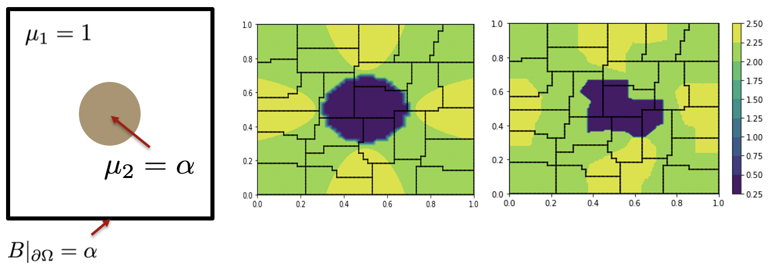
In the remainder we present results for two canonical and problems from subsurface flow and magnetostatics. In both examples we consider a cylindrical inclusion of radius embedded within the unit square centered at the origin, whose material properties are prescribed by
| (41) |
Treatment of the material interface at without interesting spurious oscillations is a hallmark of mimetic discretizations and stems for the exact treatment of interface conditions via Stokes theorem.
For both problems we will impose boundary conditions by identifying appropriate cochains on the boundary, replacing their corresponding row of the Jacobian matrix with a zero vector with one on the diagonal and setting the desired value on the right hand side. For the introductory nature of this paper this is sufficient, but we note that the imposition of boundary conditions is a rich topic in the discrete exterior calculus literature, with more complex applications requiring a deeper consideration of the interaction between boundary conditions and the discrete exterior calculus [24, 42, 12].
5.1 Problem 1: Darcy
We consider as training data solutions to the system of equations
obtained via the scheme in [50]. Boundary conditions are imposed upon the 1-cochains encoding the fluxes of through subdomain boundaries, and we stress that the resulting DEC method will guarantee that . For this problem we consider as neural network a dense elu network [23] with two hidden layers of width five, initialized with the He initializer [35]. We consider a fine mesh to generate training data.
For this problem we will consider two scenarios.
Darcy problem 1 (D1): We take and consistent with applying a unit horizontal flux and study the effect of varying . For a fixed the PDE is linear and will not require a contribution from the neural network, and we will use this to gauge the methods ability to recover a PDE discretization consistent with a single solution (i.e. ). Figure 3 provides a summary and discussion of results.


Darcy problem 2 (D2): We take and consistent with applying a horizontal flux which scales with the diffusion parameter. This corresponds to a material which becomes more conductive as the current/flux increases. To capture the nonlinear behavior of this problem will require the neural network to learn fluxes which depend upon the magnitude of the potential. Figure 4 provides a summary and discussion of results.


5.2 Problem 2: Magnetostatics
We consider as training data solutions to the system of equations
obtained via the scheme in [49]. For this 2D problem, the magnetic field may be identified with a scalar (). Boundary conditions are imposed upon the 0-cochains encoding the fluxes of through subdomain boundaries, and the 1-cochains encoding the magnetic potential on the boundary are fixed to a value of zero. For this problem we will consider only the nonlinear generalization of D2, taking and to obtain a nonlinear material whose permittivity increases with the magnitude of applied magnetic field (Figure 5. For this problem, we take as neural network a parametric ReLU activation and a single hidden layer of width ten. In the same manner as the Darcy problem, the resulting model is able to recover a range of ’s and the resulting discontinuity in the magnetic field.

6 Conclusions
We have presented a new data-driven exterior calculus which parameterizes the classical graph calculus. The resulting framework allows training of discrete exterior calculus operators which incorporates metric information from data while preserving exact sequence structure and invertibility of Hodge Laplacians - both of which are important for handling a range of physical systems. Analysis of the resulting system shows that when nonlinear perturbations are applied to a class of second-order elliptic problems the system remains well-posed under general conditions, allowing the machine learning of nonlinear elliptic systems. Numerical results demonstrate the practical aspects of the approach.
For the sake of introductory exposition, we have restricted ourselves to elementary elliptic problems in the current work. The DDEC framework however may be applied to a broad range of more sophisticated problems; for example, we are currently using it to discover surrogates for semiconductor physics governed by nonlinear drift-diffusion equations (using [47]), and where the resulting network model can be embedded within circuit simulators such as Xyce [30, 36].
Abstractly, the DDEC framework provides a structure-preserving means of parameterizing Dirichlet-to-Neumann maps [61] governing multiscale physics, generalizing previous works restricted to resistor networks [25] while supporting machine learning tasks. In future work we will provide details regarding how this may be incorporated into a workflow to develop provably stable multiscale models that preserve structure at both fine and coarse scales.
Acknowledgement
Sandia National Laboratories is a multimission laboratory managed and operated by National Technology and Engineering Solutions of Sandia, LLC, a wholly owned subsidiary of Honeywell International, Inc., for the U.S. Department of Energy’s National Nuclear Security Administration under contract DE-NA0003525. This paper describes objective technical results and analysis. Any subjective views or opinions that might be expressed in the paper do not necessarily represent the views of the U.S. Department of Energy or the United States Government.
N. Trask has also been supported by the U.S. Department of Energy, Office of Advanced Scientific Computing Research under the Collaboratory on Mathematics and Physics-Informed Learning Machines for Multiscale and Multiphysics Problems (PhILMs) project and the U.S. Department of Energy, Office of Advanced Scientific Computing Research under the Early Career Research Program. A. Huang has been supported under the Sandia National Laboratories Laboratory Directed Research and Development (LDRD) program. The work of X. Hu is partially supported by the National Science Foundation under grant DMS-1812503 and CCF-1934553.
SAND Number: SAND2020-14261 O
References
- [1] James H. Adler, Casey Cavanaugh, Xiaozhe Hu, and Ludmil T. Zikatanov. A finite-element framework for a mimetic finite-difference discretization of Maxwell’s equations. arXiv:2012.03148 [cs, math], December 2020.
- [2] Douglas Arnold, Richard Falk, and Ragnar Winther. Finite element exterior calculus: From Hodge theory to numerical stability. Bulletin of the American Mathematical Society, 47(2):281–354, 2010.
- [3] Douglas N Arnold. Finite element exterior calculus. SIAM, 2018.
- [4] Douglas N Arnold, Pavel B Bochev, Richard B Lehoucq, Roy A Nicolaides, and Mikhail Shashkov. Compatible spatial discretizations, volume 142. Springer Science & Business Media, 2007.
- [5] Douglas N. Arnold, Richard S. Falk, and Ragnar Winther. Finite element exterior calculus, homological techniques, and applications. Acta Numerica, 15:1–155, May 2006.
- [6] Nathan Baker, Frank Alexander, Timo Bremer, Aric Hagberg, Yannis Kevrekidis, Habib Najm, Manish Parashar, Abani Patra, James Sethian, Stefan Wild, et al. Workshop report on basic research needs for scientific machine learning: Core technologies for artificial intelligence. Technical report, USDOE Office of Science (SC), Washington, DC (United States), 2019.
- [7] Paul Bamberg and Shlomo Sternberg. A Course in Mathematics for Students of Physics, volume 2. 1991.
- [8] Sergio Barbarossa and Stefania Sardellitti. Topological Signal Processing over Simplicial Complexes. arXiv:1907.11577 [eess], March 2020.
- [9] Timothy Barth. On the role of involutions in the discontinuous galerkin discretization of maxwell and magnetohydrodynamic systems. In Compatible spatial discretizations, pages 69–88. Springer, 2006.
- [10] Peter Battaglia, Razvan Pascanu, Matthew Lai, Danilo Jimenez Rezende, et al. Interaction networks for learning about objects, relations and physics. Advances in neural information processing systems, 29:4502–4510, 2016.
- [11] Federico Battiston, Giulia Cencetti, Iacopo Iacopini, Vito Latora, Maxime Lucas, Alice Patania, Jean-Gabriel Young, and Giovanni Petri. Networks beyond pairwise interactions: Structure and dynamics. Physics Reports, June 2020.
- [12] René Beltman, MJH Anthonissen, and Barry Koren. Conservative polytopal mimetic discretization of the incompressible navier–stokes equations. Journal of Computational and Applied Mathematics, 340:443–473, 2018.
- [13] A Bloch. Electromechanical analogies and their use for the analysis of mechanical and electromechanical systems. Journal of the Institution of Electrical Engineers-Part I: General, 92(52):157–169, 1945.
- [14] P Bochev and A Robinson. Matching algorithms with physics: exact sequences of finite element spaces. Collected Lectures on the Preservation of Stability Under Discretization, edited by D. Estep and S. Tavener, SIAM, Philadelphia, 2001.
- [15] Pavel B Bochev, Jonathan J Hu, Christopher M Siefert, and Raymond S Tuminaro. An algebraic multigrid approach based on a compatible gauge reformulation of maxwell’s equations. SIAM Journal on Scientific Computing, 31(1):557–583, 2008.
- [16] Pavel B Bochev and James M Hyman. Principles of mimetic discretizations of differential operators. In Compatible spatial discretizations, pages 89–119. Springer, 2006.
- [17] Alain Bossavit. Computational electromagnetism: variational formulations, complementarity, edge elements. Academic Press, 1998.
- [18] Alain Bossavit. " stiff" problems in eddy-current theory and the regularization of maxwell’s equations. IEEE transactions on magnetics, 37(5):3542–3545, 2001.
- [19] Peter C Breedveld. Multibond graph elements in physical systems theory. Journal of the Franklin Institute, 319(1-2):1–36, 1985.
- [20] Michael B Chang, Tomer Ullman, Antonio Torralba, and Joshua B Tenenbaum. A compositional object-based approach to learning physical dynamics. arXiv preprint arXiv:1612.00341, 2016.
- [21] Qun Chen, Rong-Huan Fu, and Yun-Chao Xu. Electrical circuit analogy for heat transfer analysis and optimization in heat exchanger networks. Applied Energy, 139:81–92, 2015.
- [22] Fan RK Chung and Fan Chung Graham. Spectral graph theory. Number 92. American Mathematical Soc., 1997.
- [23] Djork-Arné Clevert, Thomas Unterthiner, and Sepp Hochreiter. Fast and accurate deep network learning by exponential linear units (elus). arXiv preprint arXiv:1511.07289, 2015.
- [24] Lorenzo Codecasa. Refoundation of the cell method using augmented dual grids. IEEE transactions on magnetics, 50(2):497–500, 2014.
- [25] Edward B Curtis and James A Morrow. The dirichlet to neumann map for a resistor network. SIAM Journal on Applied Mathematics, 51(4):1011–1029, 1991.
- [26] Constantine M Dafermos. Quasilinear hyperbolic systems with involutions. Archive for Rational Mechanics and Analysis, 94(4):373–389, 1986.
- [27] Mathieu Desbrun, Anil N. Hirani, Melvin Leok, and Jerrold E. Marsden. Discrete exterior calculus. 2005.
- [28] Beno Eckmann. Harmonische funktionen und randwertaufgaben in einem komplex. Commentarii Mathematici Helvetici, 17(1):240–255, 1944.
- [29] Floyd A Firestone. A new analogy between mechanical and electrical systems. The Journal of the Acoustical Society of America, 4(3):249–267, 1933.
- [30] Xujiao Gao, Andy Huang, Nathaniel Trask, and Shahed Reza. Physics-informed graph neural network for circuit compact model development. In 2020 International Conference on Simulation of Semiconductor Processes and Devices (SISPAD), pages 359–362. IEEE.
- [31] David Gilbarg and Neil S Trudinger. Elliptic partial differential equations of second order. springer, 2015.
- [32] Marco Gori, Gabriele Monfardini, and Franco Scarselli. A new model for learning in graph domains. In Proceedings. 2005 IEEE International Joint Conference on Neural Networks, 2005., volume 2, pages 729–734. IEEE, 2005.
- [33] Will Hamilton, Zhitao Ying, and Jure Leskovec. Inductive representation learning on large graphs. In Advances in neural information processing systems, pages 1024–1034, 2017.
- [34] William L Hamilton, Rex Ying, and Jure Leskovec. Representation learning on graphs: Methods and applications. arXiv preprint arXiv:1709.05584, 2017.
- [35] Kaiming He, Xiangyu Zhang, Shaoqing Ren, and Jian Sun. Delving deep into rectifiers: Surpassing human-level performance on imagenet classification. In Proceedings of the IEEE international conference on computer vision, pages 1026–1034, 2015.
- [36] S Hutchinson, E Keiter, R Hoekstra, H Watts, A Waters, T Russo, R Schells, S Wix, and C Bogdan. The xyce™ parallel electronic simulator–an overview. In Parallel Computing: Advances and Current Issues, pages 165–172. World Scientific, 2002.
- [37] Xiaoye Jiang, Lek-Heng Lim, Yuan Yao, and Yinyu Ye. Statistical ranking and combinatorial Hodge theory. Mathematical Programming, 127(1):203–244, 2011.
- [38] Xiaoye Jiang, Lek-Heng Lim, Yuan Yao, and Yinyu Ye. Statistical ranking and combinatorial hodge theory. Mathematical Programming, 127(1):203–244, 2011.
- [39] George Karypis and Vipin Kumar. Metis: A software package for partitioning unstructured graphs, partitioning meshes, and computing fill-reducing orderings of sparse matrices. 1997.
- [40] Diederik P Kingma and Jimmy Ba. Adam: A method for stochastic optimization. arXiv preprint arXiv:1412.6980, 2014.
- [41] HE Koenig and WA Blackwell. Linear graph theory-a fundamental engineering discipline. IRE Transactions on Education, 3(2):42–49, 1960.
- [42] Jasper Kreeft, Artur Palha, and Marc Gerritsma. Mimetic framework on curvilinear quadrilaterals of arbitrary order. arXiv preprint arXiv:1111.4304, 2011.
- [43] Isaac E Lagaris, Aristidis Likas, and Dimitrios I Fotiadis. Artificial neural networks for solving ordinary and partial differential equations. IEEE transactions on neural networks, 9(5):987–1000, 1998.
- [44] Lek-Heng Lim. Hodge Laplacians on Graphs. SIAM Review, 62(3):685–715, January 2020.
- [45] S. Maletić and M. Rajković. Combinatorial Laplacian and entropy of simplicial complexes associated with complex networks. The European Physical Journal Special Topics, 212(1):77–97, September 2012.
- [46] Abubakr Muhammad and Magnus Egerstedt. Control Using Higher Order Laplacians in Network Topologies. page 15, 2006.
- [47] Lawrence Musson, Xujiao Gao, Mihai Negoita, Andy Huang, and Gary L Hennigan. Charon: A radiation aware massively parallel tcad modeling code. Technical report, Sandia National Lab.(SNL-NM), Albuquerque, NM (United States), 2018.
- [48] Jean-Claude Nédélec. Mixed finite elements in . Numerische Mathematik, 35(3):315–341, 1980.
- [49] R. A. Nicolaides. Direct Discretization of Planar Div-Curl Problems. SIAM Journal on Numerical Analysis, 29(1):32–56, February 1992.
- [50] Roy A Nicolaides and Kathryn A Trapp. Covolume discretization of differential forms. In Compatible spatial discretizations, pages 161–171. Springer, 2006.
- [51] Kwang W Oh, Kangsun Lee, Byungwook Ahn, and Edward P Furlani. Design of pressure-driven microfluidic networks using electric circuit analogy. Lab on a Chip, 12(3):515–545, 2012.
- [52] Mario Ohlberger and Stephan Rave. Reduced basis methods: Success, limitations and future challenges. arXiv preprint arXiv:1511.02021, 2015.
- [53] Alfio Quarteroni, Andrea Manzoni, and Federico Negri. Reduced basis methods for partial differential equations: an introduction, volume 92. Springer, 2015.
- [54] Maziar Raissi, Paris Perdikaris, and George E Karniadakis. Physics-informed neural networks: A deep learning framework for solving forward and inverse problems involving nonlinear partial differential equations. Journal of Computational Physics, 378:686–707, 2019.
- [55] Maziar Raissi, Paris Perdikaris, and George Em Karniadakis. Physics informed deep learning (part i): Data-driven solutions of nonlinear partial differential equations. arXiv preprint arXiv:1711.10561, 2017.
- [56] Frank Rosenblatt. Principles of neurodynamics. perceptrons and the theory of brain mechanisms. Technical report, Cornell Aeronautical Lab Inc Buffalo NY, 1961.
- [57] Kevin Scaman and Aladin Virmaux. Lipschitz regularity of deep neural networks: Analysis and efficient estimation. arXiv:1805.10965 [cs, stat], October 2019.
- [58] Michael T. Schaub, Austin R. Benson, Paul Horn, Gabor Lippner, and Ali Jadbabaie. Random Walks on Simplicial Complexes and the Normalized Hodge 1-Laplacian. SIAM Review, 62(2):353–391, January 2020.
- [59] S. Smale. On the mathematical foundations of electrical circuit theory. J. Differential Geom., 7(1-2):193–210, 1972.
- [60] Malcolm C Smith. Synthesis of mechanical networks: the inerter. IEEE Transactions on automatic control, 47(10):1648–1662, 2002.
- [61] John Sylvester and Gunther Uhlmann. The dirichlet to neumann map and applications. In Inverse problems in partial differential equations, volume 42, page 101. SIAM Publications, Philadelphia, 1990.
- [62] Joaquín J. Torres and Ginestra Bianconi. Simplicial complexes: Higher-order spectral dimension and dynamics. Journal of Physics: Complexity, 1(1):015002, May 2020.
- [63] Nikolaos Vlassis, Ran Ma, and WaiChing Sun. Geometric deep learning for computational mechanics part i: Anisotropic hyperelasticity. arXiv preprint arXiv:2001.04292, 2020.
- [64] Sifan Wang, Yujun Teng, and Paris Perdikaris. Understanding and mitigating gradient pathologies in physics-informed neural networks. arXiv preprint arXiv:2001.04536, 2020.
- [65] Sifan Wang, Xinling Yu, and Paris Perdikaris. When and why pinns fail to train: A neural tangent kernel perspective. arXiv preprint arXiv:2007.14527, 2020.
- [66] Hermann Weyl. Repartición de corriente en una red conductora. Revista Matemática Hispano-Americana, 5:153–164, 1923.
- [67] Herbert S. Wilf and Frank Hilary. "Mathematical aspects of electrical network analysis", volume 3 of SIAM-AMS proceedings. American Mathematical Society, 1971.
- [68] Kane Yee. Numerical solution of initial boundary value problems involving maxwell’s equations in isotropic media. IEEE Transactions on antennas and propagation, 14(3):302–307, 1966.