∎
Learning from What We Know
Abstract
Vulnerability prediction refers to the problem of identifying system components that are most likely to be vulnerable. Typically, this problem is tackled by training binary classifiers on historical data. Unfortunately, recent research has shown that such approaches underperform due to the following two reasons: a) the imbalanced nature of the problem, and b) the inherently noisy historical data, i.e., most vulnerabilities are discovered much later than they are introduced. This misleads classifiers as they learn to recognize actual vulnerable components as non-vulnerable. To tackle these issues, we propose TROVON, a technique that learns from known vulnerable components rather than from vulnerable and non-vulnerable components, as typically performed. We perform this by contrasting the known vulnerable, and their respective fixed components. This way, TROVON manages to learn from the things we know, i.e., vulnerabilities, hence reducing the effects of noisy and unbalanced data. We evaluate TROVON by comparing it with existing techniques on three security-critical open source systems, i.e., Linux Kernel, OpenSSL, and Wireshark, with historical vulnerabilities that have been reported in the National Vulnerability Database (NVD). Our evaluation demonstrates that the prediction capability of TROVON significantly outperforms existing vulnerability prediction techniques such as Software Metrics, Imports, Function Calls, Text Mining, Devign, LSTM, and LSTM-RF with an improvement of 40.84% in Matthews Correlation Coefficient (MCC) score under Clean Training Data Settings, and an improvement of 35.52% under Realistic Training Data Settings.
Keywords:
vulnerability prediction trovon training on vulnerabilities only encoder-decoder machine translation tf-seq2seq1 Introduction
A vulnerability is a hole or a weakness in the application, which can be a design flaw or an implementation bug, that allows an attacker to cause harm to the stakeholders, i.e., the application owner, application users, and other entities that rely on the application Vulnerabilities. While vulnerabilities can be thought of as specific types of software defects (or bugs), there are subtle and significant differences that make their identification considerably more complex and challenging than the problem of finding bugs TangZYLZX15; PotterMcGraw2004.
Vulnerabilities are fewer in comparison to defects, limiting the information one can learn from. Also, their identification requires an attacker’s mindset Morrison+2015, which developers or code reviewers may not possess. Lastly, the continuous growth of codebases makes it difficult to investigate them entirely and track all code changes. For example, the Linux kernel, one of the projects with the highest number of publicly reported vulnerabilities, reached 27.80 million LoC (Lines of Codes) at the beginning of 2020 linux-news.
Vulnerability prediction approaches were proposed to tackle these challenges by prioritizing the efforts that developers and code reviewers have to put on when testing or reviewing code to find vulnerabilities. These methods take advantage of the large amounts of historical data available based on which they learn a set of features and/or code properties that associate with vulnerabilities. For instance, the presence of vulnerabilities has been linked to high code churn ShinMWO2011, to the use of specific library imports and function calls Neuhaus+2007, and the frequency of suspicious code tokens TangZYLZX15. Unfortunately, building models around such features is challenging due to the small number of available vulnerable code instances, which limit the learning ability of the predictors Zimmermann+2009.
Furthermore, Jimenez et al.Jimenez+2019 demonstrated that vulnerability prediction approaches have been built under a “clean” training data assumption, i.e., all the component’s labeling information (vulnerable / non-vulnerable) is always available irrespective of time. Their study showed that under these settings the approaches do not account for the gradual revelation of vulnerabilities over time. This results in prediction models training on even those vulnerabilities that have not been uncovered yet, e.g., all vulnerabilities known from time t onwards are available at all times, even before time t.
Jimenez et al.advocated Realistic Training Data Settings where the vulnerability labels used for training the prediction models are more realistically available at training time. For example, in such settings, at a given time t, only the vulnerabilities known till time t should be available for training. All vulnerabilities known from time t onwards should not be available for training beforehand. Their study demonstrated that Realistic Training Data Settings results in unavoidable noise in the training data because every component with no reported vulnerability till training time is considered non-vulnerable during training, which makes existing approaches perform poorly. This establishes a need for robust vulnerability prediction techniques.
We advance in this direction by developing TROVON 11 1 TROVON is an abbreviation for “Training on vulnerabilities only”, which is the core focus of our study.– a method that learns from validated data, i.e., we train only on components known to be vulnerable and leave aside the (supposedly) non-vulnerable ones. This way, we do not make any assumptions on non-vulnerable components and bypass the key problem faced by previous works. To do so, we rely on a simple yet powerful language-agnostic machine translation technique Britz:2017 which we train on pairs of vulnerable and fixed code fragments, available at projects’ release time. In particular, we contrast the code fragments pairs (pairs of vulnerable and fixed fragments) that were modified when fixing a vulnerability, with fragment pairs from other functions of the same components (fragments less likely to be vulnerable) in order to learn to distinguish likely vulnerable from non-vulnerable code.
TROVON focuses on vulnerability fixes, i.e., code transformations that turn vulnerable code into a non-vulnerable one, to train the machine translation model that aims at capturing silent features related to the differences between vulnerable and fixed components. Therefore, predictions are guided by actual points of interest, (i.e., diff points) in the vulnerable code where the transformations should happen. This means that TROVON learns to identify code characteristics that are similar to those (vulnerable) seen during training.
We empirically assess the effectiveness of TROVON on available releases of three security-critical open source systems, i.e., Linux Kernel, Wireshark, and OpenSSL. Our evaluation demonstrates that TROVON significantly outperforms existing vulnerability prediction approaches under both Clean Training Data Settings and Realistic Training Data Settings.
In particular, our results show that when we train all the approaches (including TROVON) with clean training data, TROVON outperforms the existing approaches by 83.96% in Precision, 155.33% in Recall, 132.95% in F-measure, and 80.39% in Matthews Correlation Coefficient (MCC). In addition to these metrics, we also evaluate TROVON on predicting unseen vulnerable components specifically. This is a new metric that we introduce in this paper to help evaluate the extent to which vulnerability prediction generalizes, i.e., ability to predict unseen components (components not used for training) as being vulnerable or not. The percentages of unseen vulnerable components predicted by TROVON, on average, are 40.05%, 64.34%, and 42.28% higher than the ones obtained by existing techniques in Linux Kernel, Wireshark, and OpenSSL releases, reflecting TROVON’s better generalization capability. Under Realistic Training Data Settings, on average, TROVON achieved 0.39 MCC, (i.e., 3.63 times higher than the baselines), 0.69 F-measure, (i.e., 11.82 times higher), 0.86 Precision, (i.e., 2.66 times higher), and 0.58 Recall, (i.e., 15.25 times higher than the baselines).
In summary, we make the following contributions:
- 1.
We present TROVON, a novel vulnerability prediction method via machine translation.
- 2.
We demonstrate that TROVON significantly outperforms existing methods through a large empirical study.
- 3.
We corroborate that TROVON remains robust when trained in Realistic Training Data Settings that includes unavoidable noise, where almost all previous methods that we compared with, fail Jimenez+2019.
2 Background
2.1 Vulnerabilities
Common Vulnerability Exposures (CVE) CVE:Terminology defines a security vulnerability as “a mistake in software that can be directly used by a hacker to gain access to a system or network”. The inadvertence of a developer or insufficient knowledge of defensive programming usually causes these mistakes. Still, vulnerabilities are of critical importance for software vendors, who often offer bounties to find them and prioritize their resolution over other less harmful bugs, hence reducing a potential business impact.
Vulnerabilities are usually reported in publicly available databases to promote their disclosure and fix. One such example is National Vulnerability Database, aka NVD NVD. NVD is the U.S. government repository of standards based vulnerability management data. All vulnerabilities in the NVD have been assigned a CVE (Common Vulnerabilities and Exposures) identifier. The Common Vulnerabilities and Exposures (CVE) Program’s primary purpose is to uniquely identify vulnerabilities and to associate specific versions of codebases (e.g., software and shared libraries) to those vulnerabilities. The use of CVEs ensures that two or more parties can confidently refer to a CVE identifier (ID) when discussing or sharing information about a unique vulnerability. For every vulnerability, along with the Git commit IDs of the code related to vulnerability-fix commit, NVD also provides related information, i.e., CVE number, vulnerability description, CWE number (if applicable), time of creation, and the list of the impacted releases in the form of reports.
2.2 Vulnerability Prediction Modeling
2.2.1 Prediction modeling
Prediction modeling aims at learning statistical properties of interest based on historical data. While the resulting models are usually suitable only for the project/application on which they have been trained, the learning process is generic and applies to a specific set of features that associate with the property to predict. In the context of vulnerabilities, a prediction model can be used to classify software components as likely or unlikely vulnerable. This information can be used to support the code review process. The task is similar to defect prediction, yet due to the sparsity of available examples, it is harder to predict vulnerabilities than defects shin_can_2013; TheisenW20.
2.2.2 Intra vs Inter Predictions:
Prediction modeling is usually performed in both intra- and cross-project fashion, i.e., training on data of the same or of other projects. However, vulnerabilities are project-specific, i.e., they are tied to the project context, used libraries, and development process, and thus, inter-project predictions do not work. Scandariato et al. 6860243 found that the models for 11 apps out of 20 were too specific for cross-project prediction, and that the link was more pairwise rather than generic. The results of cross-project vulnerability prediction in the study of Sara et al. DBLP:conf/sac/MoshtariS16 show high recall but comparatively low F2 using coupling and IVH. Therefore, research in this area is focussed on intra-project.
2.3 Granularity Level
Prediction models can target various levels of granularity, such as line, function, component, etc. However, the key target should be actionable for the developers and code reviewers that are envisioned to use the technique. Given this, a commonly accepted tradeoff is the component (file) level granularity as it has been vetted by Microsoft developers in a study of Morrison et al.Morrison+2015, and is used by most existing approaches. Thus, we consider a code-file as our component, i.e., file-level granularity, as it is actionable for industrial use Morrison+2015, and provides a baseline for comparing our results with those reported in the relevant literature that we elaborate in Section 4.5.
2.4 Clean Training Data Settings
Jimenez et al.Jimenez+2019 demonstrated that the existing vulnerability prediction approaches have been built under a “clean” training data assumption, i.e., all the component’s labeling information (vulnerable / non-vulnerable) is always available irrespective of time, which is unrealistic. Jimenez et al.showed that under these settings, aka Clean Training Data Settings, prediction approaches fail to account for the gradual revelation of vulnerabilities over time. This results in biased prediction models, i.e., models trained on vulnerabilities that have not been been discovered at the release time, e.g., all vulnerabilities known from time t onwards are available at all times, even before time t.
2.5 Realistic Training Data Settings
In contrast to Clean Training Data Settings, where the component’s labeling information (vulnerable / non-vulnerable) is always available irrespective of time, Realistic Training Data Settings necessitate vulnerability labels to be used for training the prediction models to be those that are available at training time. For instance in Realistic Training Data Settings, at a given time t, only the vulnerabilities known at time t should be available for training. All vulnerabilities known after time t should not be available for training beforehand. Jimenez et al.study demonstrated that Realistic Training Data Settings introduce noise in the training data, because every component with no reported vulnerability till the training time is considered as non-vulnerable during training, that makes existing approaches perform poorly.
Irrespective of the poor performance of existing approaches, Realistic Training Data Settings represents a realist case study, the vulnerabilities are discovered and fixed long after the release date of the projects. In our release-based experiments, (i.e., one release for training the model and next release for testing the trained model), only those components are considered as vulnerable in the training set whose vulnerabilities have been discovered and fixed before the next release date of the system.
2.6 Seen Vulnerable Components
Vulnerabilities can remain in the code and get propagated throughout different releases (one release after another) of a system, without getting fixed. Due to this, in a release-based experiment, (i.e., one release for training the model and next release for testing the trained model), vulnerable components that are present in the training set and “seen” by the prediction model during training can also appear in the testing set. Throughout our paper, we refer to such components as Seen vulnerable components.
2.7 Unseen Vulnerable Components
From one release of a system to the next one, many files/components are modified either to introduce a new functionality or to modify an existing one. In case of Linux Kernel, Wireshark, and OpenSSL projects, we analyzed that 29.95%, 72.53%, and 73.58% of the files, on average, are changed between the releases. A component that was non-vulnerable in the previous release can be become vulnerable in this release, because of such a modification by a developer. Due to this, in a release-based experiment, any component in a testing set which is vulnerable and is not available in the training set, represents a novel vulnerability. Since, this component is “unseen” and has not been trained on by the model, we refer to it as Unseen vulnerable component.
2.8 Machine Translation
We perform vulnerability prediction using Machine Translation. Machine Translation can be considered as a transformation function , where the input is a set of entities that represents a component to be transformed to produce the output , which is a set of entities that represent a desired component.
In the training phase, the transformation function learns on the example pairs available in the training dataset. In our context, contains vulnerable entities, representing a vulnerable component, and contains fixed entities, representing the corresponding fixed component. The transformation function can be trained not to transform, i.e., to reproduce the same output as the input in cases where is the desired entity-set. This is achieved by training the function on the example pairs , i.e. . In the case of vulnerability prediction modeling, this learned transformation will be used as our prediction model.
2.9 RNN Encoder-Decoder architecture
The encoder-decoder architecture for recurrent neural networks is the standard neural machine translation method that rivals and in some cases outperforms classical statistical machine translation methods rnnencoderdecoder. We use the RNN Encoder-Decoder that is established and is used by many recent studies garg2022cerebro; sutskever2014sequence; Tufano_2019. The RNN Encoder-Decoder machine translation is composed of two major components: RNN Encoder to encode a sequence of terms into a vector representation, and RNN Decoder to decode the representation into another sequence of terms . The model learns a conditional distribution over an output sequence conditioned on another input sequence of terms: , where and may differ. For example, given an input sequence = = and a target sequence = = , the model is trained to learn the conditional distribution: , where and are separated tokens. A bi-directional RNN Encoder Britz:2017, formed by a backward RNN and a forward RNN, is considered the most efficient to create representations as it takes into account both past and future inputs while reading a sequence bahdanau2014neural.
3 Approach
The key idea of TROVON is to train a machine translator (viz. an encoder-decoder sequence to sequence model) to identify vulnerable code, by feeding it with vulnerable code fragments and their corresponding fixes. Machine translators can automatically recognize: (i) features of the language (to be translated) and (ii) required translation (to the desired language). In our case, it is used to automatically identify vulnerability features with minimum overhead.
It should be noted that we do not aim at fixing vulnerable code, but rather at identifying likely vulnerable code instances. The point here is that we use the translator to indicate the presence of vulnerabilities without considering the fixes produced by the model. In other words, we leverage the ability of the translators to learn the vulnerabilities’ context and not their instance and location. We assert that since vulnerable code instances are scarce, information gained from historical data is inevitably partial and incomplete. Therefore, it can be used to indicate the presence of vulnerabilities but not their instance context.
The translator is trained on input - desired output pairs,i.e., on vulnerable - fixed code fragments. For prediction, one can input an unseen code into the trained translator to check whether it is likely to be vulnerable. If the translator changes the code then it can be concluded that the code is likely to be vulnerable. To avoid many false positives (the translator changing every input code fragment), we also train it to leave non-vulnerable code fragments unchanged. To this end, we also feed the translator with input-output pairs where each of which is a non-vulnerable code fragment (input = output). It must be noted that we train only on the components (files) that were fixed, leaving aside the unchanged ones. This way we aim at reducing the noise from the training data, i.e., by focusing on what we are certain of; the information provided by the vulnerability fixes.
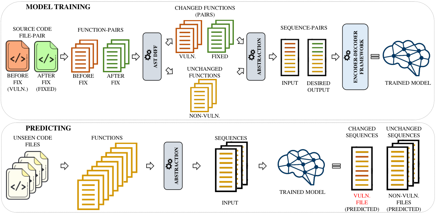
Figure 1 shows an overview of the implementation. Starting from vulnerable code components and their fixes, it involves the following activities: 1) decomposing the components into code fragments; 2) identifying which code-fragments are responsible for the vulnerability; 3) producing abstracted code-fragments by removing irrelevant information (e.g. user-defined names, comments); 4) configuring and training the machine translator. 5) producing abstracted code-fragments of an unseen code component and using the trained machine translator to predict whether it is likely to be vulnerable.
3.1 Decomposing Components into Code Fragments
We target our predictions at the component, (i.e., file) level due to: a) the empirical evidence provided by Morrison et al.Morrison+2015 and b) to account for the context of code (vulnerability-fixes) that can be fixed at multiple locations throughout the component. A code-fix can be an addition, removal, and/or modification of code. Since functions are the basic building blocks of a program, we use them to establish function-level mappings between the vulnerable components and their fixed counterparts (based on the function headers).
Thus, we extract all the functions from both, a vulnerable component and its fixed counterpart, and pair each before-fix function with the corresponding after-fix function. The functions that cannot be paired, i.e., having no counterpart, are discarded. This can happen due to the creation and/or deletion of a function to fix a vulnerability, e.g., a function added during the fix which was not present before or vice-versa.
3.2 Categorizing Functions as Vulnerable or Non-Vulnerable
As typically performed in this line of work, we consider as vulnerable, any function that was modified to fix the vulnerability. The remaining are considered as non-vulnerable (not vulnerable to the specific vulnerability). When comparing a before-fix copy to its after-fix counterpart, we ignore irrelevant syntactical changes, e.g., additional blank spaces and new lines. If there remain syntactical differences between the two copies, we label the before-fix as vulnerable.
3.3 Abstracting Irrelevant Information
A major challenge in dealing with raw source code is the huge vocabulary created by the abundance of identifiers and literals used in the code. Vocabulary, on such a large scale, hinders the learning of relevant code patterns Tufano_2019. Thus, to reduce the vocabulary size, we transform the source code into an abstract representation by replacing user-defined entities with re-usable IDs.
Figure 2 shows a code snippet of a real function (Figure 2(a)) converted into its abstract representation (Figure 2(b)). The purpose of this abstraction is to replace any reference to user-defined entities (function name, type name, variable name, and string literal) with IDs that can be reused across functions (thereby reducing vocabulary size). Thus, we replace identifiers and string literals with unique IDs. Additionally, comments and annotations are removed.
New IDs follow the regular expression (F|T|V|L)_(num)+, where num stands for numbers assigned in a sequential and positional fashion based on the occurrence of that entity. All the entities - user-defined Function names, Type names, Variable names, and String Literals are replaced with F_num, T_num, V_num, and L_num, respectively. Thus, the first function name receives the ID F_1, the second receives the ID F_2, and so on. If any of these entities appear multiple times in a function, it is replaced with the same ID.
Each function (pair) is abstracted in isolation to yield an abstracted function code, i.e., same IDs can be reused across functions without impacting TROVON. ID references are not preserved across functions, e.g., V_1 may refer to two different variable names from one function to another. This is the key to reduce the vocabulary size, e.g., the name of the first function called in any pair is replaced with the ID F_1, regardless of its original name.
In the case of vulnerable functions, the before-fix copy is abstracted first and then the after-fix copy. IDs are shared between the two copies (before-fix and after-fix) of the functions and new IDs are generated only when new (Function, Type, Variable) names and String Literals are found.
The abstracted code is rearranged in a single sentence to represent a sequence of space-separated entities, which is the representation supported by the machine translator. Sequences generated from vulnerable (before-fix), fixed (after-fix), and unchanged functions are named vulnerable, fixed, and unchanged sequences, respectively. In these settings, fixed and unchanged sequences represent non-vulnerable cases. To limit the computation cost involved in training the translator, large sequences are split into multiple sequences of no more than 50 tokens each.
3.4 Building the Machine Translator
To build our machine translator, we train an encoder-decoder model that can transform an input sequence to the desired sequence (output of the model).
A representation of a sequence is similar to a sentence in a natural language that consists of words separated by spaces and ends with a full stop. Instead of words and full stop character, a sequence has tokens and a newline character. Thus, we train the encoder-decoder by feeding it with pairs of sequences. More precisely, we use two types of pairs: (i) vulnerable sequences with their corresponding fixed sequences, and (ii) non-vulnerable sequences paired with themselves. Non-vulnerable sequence-pairing is essential to allow the learner to identify what should not be changed. Thereby, avoiding to raise many false positives (incorrectly predicting non-vulnerable sequences as vulnerable) while learning only from “clean” data.
3.5 Predicting Vulnerable Components
To predict whether an unseen component, (i.e., file) is potentially vulnerable, we decompose it into sequences following the process depicted in Figure 1. Then, we feed the resulting sequences into the machine translator which produces output sequences. If one (or more) of the output sequences returned by the model is different from the original one, (i.e., input sequences), we consider the component as likely to be vulnerable. Otherwise, we consider component as likely non-vulnerable, i.e., in case of no change in any of the output sequences in comparison to the input sequences, the component is considered as likely non-vulnerable.
4 Experimental Evaluation
4.1 Research Questions
TROVON aims to support code reviews by predicting vulnerable components in new releases, based on the information learned from previous (historical) data, i.e., the previous project release. Therefore, our first research question regards the prediction ability of TROVON. We measure the prediction ability of TROVON to correctly predict vulnerable and non-vulnerable components. We do so with the help of classification assessment metrics, i.e., Precision, Recall, F-1, and MCC. We evaluate this by training on all available vulnerabilities of one release and testing on the next release, for all available release pairs. Thus, we ask:
- RQ1
What is the prediction performance of TROVON in a release-based scenario ?
After assessing the prediction ability of TROVON, we turn our attention to existing techniques. Hence, we investigate:
- RQ2
What is the prediction performance of TROVON in comparison to existing techniques?
In TROVON, we train a model on the vulnerabilities of a release and test the trained model on the components of the next release. Since we perform a release-based evaluation, vulnerabilities spanning across multiple releases could be either seen by the trained model (used during training) or not (newly appearing component). Thus, we may have the knowledge in advance that a component is vulnerable in a given release irrespective of the vulnerability detection date. As these vulnerable components may remain unfixed and reappear in the next release, it is essential to assess the learning potential of our models by evaluating how proficient are the studied models in classifying correctly components that were “seen” during training, in a sense checking how well the model remembers, and in classifying new components, i.e., components that were “unseen” during training, in a sense checking how well a model can actually perform on new instances. Hence, we aim at controlling for seen and unseen vulnerable components and ask:
- RQ3
What is the prediction performance of the studied techniques in predicting seen and unseen vulnerable components?
Until now, we consider that in every release all known vulnerable components are labelled as such, i.e., following the clean training data settings. This analysis provides indications on what the potential prediction ability of the approaches is when the available data are clean, i.e., all the component’s labeling information (vulnerable / non-vulnerable) is always available irrespective of time. Unfortunately, in practice, such information is unavailable and inflates the actual performance of the prediction models. The actual performance in Realistic Training Data Settings is much lower due to real-world labeling issues Jimenez+2019, i.e., vulnerabilities are frequently reported at a much later time than they are actually introduced. This has adverse effects as they cause the classifiers to treat vulnerable components as non-vulnerable. Hence, it is imperative to study performance under Realistic Training Data Settings, where a prediction model is trained only on those vulnerabilities that were detected till the release date of a version for which the vulnerability prediction is performed. For this reason, we also evaluate the approaches under Realistic Training Data Settings. Hence, we ask:
- RQ4
How effective (in predicting vulnerable components) is TROVON in comparison to existing techniques under Realistic Training Data Settings?
4.2 Data
For our study, we need projects with many releases and vulnerabilities. We consider three large security-intensive open-source systems that were used by previous research Jimenez+2019 – the Linux Kernel, the OpenSSL library, and the Wireshark tool. These systems are widely used, mature, and have a long history of releases and vulnerability reports.
Linux Kernel LinuxKernel is an operating system, integrated into billions of systems and devices, such as Android. Linux is one of the largest open-source code-bases and has a long history (since 1991), recorded in its repository. It is relevant for our evaluation since it has many security aspects and is among the projects with a higher number of reported vulnerabilities in NVD. OpenSSL OpenSSL is a library implementing the SSL and TLS protocols, commonly used in communications. It is of critical importance as highlighted by the Heartbleed vulnerability, which made half of a million web servers vulnerable to attacks heartbleed. Wireshark WireShark is a network packet analyzer mainly used for troubleshooting and debugging. The project is open source and is relevant for the study because it is integrated with most operating systems.
We use VulData7 JimenezPT18 which is a publicly available22 2 https://github.com/electricalwind/data7 tool to gather the vulnerabilities, i.e., the vulnerable and the corresponding fixed components of the aforementioned systems. As we mention in section 2.1, for every vulnerability, NVD provides a Git commit IDs of the code related to vulnerability-fix commit. By using these NVD provided Git commitIDs, VulData7 extracts the code of vulnerabilities, (i.e., vulnerable code and its patch) and creates a vulnerability dataset.
To gather the code-base of these systems, we use FrameVPM Jimenez+2019 which is also a publicly available tool33 3 https://github.com/electricalwind/framevpm. FrameVPM is a framework built to evaluate and compare vulnerability prediction models. We also used FrameVPM to perform a prediction comparison with existing techniques. Section 4.5 elaborates on the re-implementation of existing techniques that we compare with. Table 1 provides the details of our dataset. The dataset composed of the vulnerabilities reported in National Vulnerability Database (NVD) NVD, and the codebase gathered for the 36 releases of Linux Kernel project LinuxKernel, 10 releases of Openssl project OpenSSL, and 10 releases of Wireshark project WireShark is publicly available44 4 https://github.com/garghub/TROVON, along with our source-code and our re-implemented source-code of the baselines that we compared TROVON with.
| System | #Releases | #Avg.Comp | #Avg.Vuln.Comp | %Vuln. |
| Linux Kernel | 36 | 16456 | 456 | 3% |
| Wireshark | 10 | 2012 | 134 | 7% |
| OpenSSL | 10 | 664 | 59 | 9% |
4.3 Implementation and Model Configuration
During the abstraction phase, we rely on the srcML tool 7816536 to convert source code into an XML format including tags to identify literals, keywords, identifiers, and comments. This helps in separating user-defined identifiers and string literals (the largest part of the vocabulary) from language keywords (a limited set). Then, ID replacement is performed by a dedicated tool that we implemented. To check whether before and after-fix copies are different, we input the XML produced by srcML into the Gumtree Spoon AST Diff falleri:hal-01054552 tool. The purpose of using Gumtree Spoon AST Diff is to achive a fine-grained diff which can ignore irrelevant changes such as whitespaces and/or new line characters. It should be noted that TROVON is not bound to the above-mentioned third-party tools. As an alternative, one can use any utility that identifies user-defined entities and performs a diff.
Our encoder-decoder model is built on top of tf-seq2seq tensorflow2015-whitepaper, a general-purpose encoder-decoder framework. To configure it, we learn from previous works that apply machine translation to solve software engineering tasks other than vulnerability prediction, e.g., Tufano_2019; DBLP:journals/tosem/TufanoWBPWP19; garg2022cerebro. Thus, we rely on a bidirectional encoder as it generally outperforms a unidirectional encoder bahdanau2014neural. We use a Long Short-Term Memory (LSTM) network HochreiterHochreiter1997 to act as the Recurrent Neural Network (RNN) cell, which was shown to perform better than other common alternatives like simple RNNs or gated recurrent units, in other software engineering prediction tasks lstmcomparison2019; lstmcomparisonwebsite. Bucketing and padding are used to deal with the variable length of sequences. To strike a balance between performance and training time, we utilize AttentionLayerBahdanau as our attention class, configured with 2 layered AttentionDecoder and 1 layered BidirectionalRNNEncoder, both with 256 units.
To determine an appropriate number of training steps, we conducted a preliminary study involving a validation set (independent of both the training set and the test set that we use in our experimental evaluation) and trained the model by iterations of 5,000 steps. At the end of each iteration, we check whether the prediction accuracy on the validation set improved. If it improved, then we pursued the training for another iteration, otherwise, stopped. We found out that the model stopped improving at 50,000 steps, which we thus set as a threshold. This order of magnitude is in line with previous research applying machine translation to solve software engineering prediction tasks, e.g., garg2022cerebro; Tufano_2019.
4.4 Experimental Settings
Our experimental evaluation is designed to evaluate techniques under Clean Training Data Settings and Realistic Training Data Settings. We train a model on each release and test the trained model on the following release, (i.e., next release) simulating a typical release-based vulnerability prediction evaluation scenario Jimenez+2019.
Clean Training Data Settings - Used in RQs 1, 2 & 3: In these settings, a prediction model is trained using all the vulnerabilities (vulnerable, i.e., before-fix sequences transformation to non-vulnerable, i.e., after-fix sequences) of a release of a system (Linux Kernel / OpenSSL / Wireshark). The trained models are evaluated based on their predictions in the following release of the same system (e.g., trained on vulnerable components in Linux Kernel release v4.0 and evaluated on all components of v4.1). The components of the following release are converted into sequences that are input to the trained model to get the output sequences. Then, TROVON compares the output sequences generated by the trained model with the input sequences. A component is considered vulnerable if any of the output sequences differ from the input sequences, otherwise considered as non-vulnerable. This training-testing process is repeated for all available releases.
For our release-based experiments where we train the models of different approaches on one release and test the trained models on the next release, in total we have 36 releases of Linux Kernel, 10 releases of Wireshark, and 10 releases of OpenSSL, as mentioned in Table 1. In case of (n) releases available to us for a system, we can only perform (n–1) experiments because in chronological order, the last experiment would be to train a model on (n–1)th release and test the trained model on (n)th release. The reason for such is that we do not have a release to test a model trained on the nth release. Hence, for 1 approach, we performed 35 experiments for Linux Kernel, 9 experiments for Wireshark, and 9 experiments for Wireshark. That results to 53 experiments in total (35 + 9 + 9 = 53), for 1 approach.
Realistic Training Data Settings - Used in RQ4: In contrast to the clean training data settings, in Realistic Training Data Settings we consider the date when the vulnerability was fixed. Vulnerability fixing date determines whether a vulnerability is included in the training dataset or not. In these settings, a prediction model (for one release of the system) is trained only on those vulnerabilities that were fixed before the next release date. Then, the trained model is evaluated on all the components of the following release of the same system.
4.5 Benchmarks for Vulnerability Prediction
To assess effectiveness, we compare TROVON with existing vulnerability prediction techniques. To perform the comparison we use FrameVPM, a framework enabling the replication and comparison of vulnerability prediction approaches, introduced by Jimenez et al.Jimenez+2019. Overall, we compare TROVON with:
Software Metrics: Complexity metrics have been extensively used for defect prediction (e.g. Hall+2012) and vulnerability prediction (e.g. 10.1145/1414004.1414065; ShinMWO2011; 10.1016/j.sysarc.2010.06.003; TheisenW20). It is based on the idea that complex code is difficult to maintain and test, and thus has a higher chance of having vulnerabilities than simple code. Using FrameVPM, we replicate and compare with the original study from Shin et al.ShinMWO2011 that rely on features related to following metrics:
- 1.
Complexity and Coupling
- (a)
LinesOfCode: lines of code;
- (b)
PreprocessorLines: preprocessing lines of code;
- (c)
CommentDensity ratio: lines of comments to lines of code;
- (d)
CountDeclFunction: number of functions defined;
- (e)
CountDeclVariable: number of variables defined;
- (f)
CC(sum, avg, max): sum, average and max cyclomatic complexity;
- (g)
SCC(sum, avg, max): strict cyclomatic complexityShinMWO2011;
- (h)
CCE(sum, avg, max): essential cyclomatic complexityShinMWO2011;
- (i)
MaxNesting(sum, avg, max): maximum nesting level of control constructs;
- (j)
fanIn(sum, avg, max): number of inputs, i.e., input parameters and global variables to functions;
- (k)
fanOut(sum, avg, max): number of outputs, i.e., assignments to global variables and parameters of function calls.
- (a)
- 2.
Code Churn: added lines, modified lines and deleted lines in the history of a component.
- 3.
Developer Activity Metrics:
- (a)
number of commits impacting a component;
- (b)
number of developers modified a component;
- (c)
current number of developers working on a component.
- (a)
Text Mining: It considers a source code component as a collection of terms associated with frequencies, also known as Bag of Words (BoW), used for vulnerability prediction 6860243. The source code is broken into a vector of code tokens, and the frequency of each token is then used as the features to build the vulnerability prediction model. Further improvements have been performed to significantly improve its performance, e.g., by pooling frequency values in different bins according to particular criteria to discretize BoW’s features 6860243; 10.5555/1643031.1643034; TheisenW20.
Imports and Function Calls: The work of Neuhaus et al. Neuhaus+2007 is based on the observation that the vulnerable components tend to import and call a particular small set of functions. Thus, the features of this simple prediction model are the components’ imports and function calls. Following the suggestions of FrameVPM, we use imports and function calls as separate sets of features. We train one model based on Imports and another based on Function Calls, thus implementing one model per set of features.
Devign: The work of Zhou et al. zhou2019devign emphasizes the use of graph neural network for vulnerability detection. With Abstract Syntax Tree (AST) as the backbone, Zhou et al. proposed to convert components (vulnerable/non-vulnerable) as code property graphs which helps to solve the problem of information loss during learning. To perform component classification, (i.e., graph-level classification), graph neural network models are trained which are composed of gated graph recurrent layer and convolutional layer, that enables to learn the vulnerable programming pattern. Since the authors’ implementation of the approach is not available, we implemented Devign based on our understanding of zhou2019devign and made it publicly available55 5 https://github.com/garghub/TROVON/tree/main/devign.
LSTM and LSTM-RF: The work of Dam et al. Dam+2018 focuses to capture semantic features of code components (vulnerable/non-vulnerable) and using these features to perform vulnerability prediction. Dam et al. asserted that Long Short Term Memory (LSTM) HochreiterHochreiter1997 is highly effective in learning long-term dependencies in sequential data such as text and speech, and can be used to learn features that represent both the semantics of code tokens (semantic features) and the sequential structure of source code (syntactic features). In this approach, components are encoded using the embedding layer, and along with labels (vulnerable/non-vulnerable), are used to train LSTM models. Although these trained LSTM models are capable of prediction, i.e., to provide a probability of a component being vulnerable, the approach extends a step further. The embeddings for the components are extracted using the trained LSTM models, and are used to train binary classifier. Finally, the trained binary classifier provides the probability/likelihood of a component being vulnerable. For LSTM approach, we used the trained LSTM models for predictions, and for LSTM-RF approach, we used trained binary classifiers for predictions. Here as well, due to unavailable authors’ implementation, we implemented the approach based on our understanding of HochreiterHochreiter1997 and made it publicly available66 6 https://github.com/garghub/TROVON/tree/main/lstm-rf.
4.6 Performance measurement
Vulnerability prediction modeling is a binary classification problem, thus it can result in four types of outputs: Given a vulnerable component, if it is predicted as vulnerable, then it is a true positive (TP); otherwise, it is a false negative (FN). Given a non-vulnerable component, if it is predicted as non-vulnerable, then it is a true negative (TN); otherwise, it is a false positive (FP). From these, we can compute the traditional evaluation metrics such as Precision, Recall, and F-measure scores, which quantitatively evaluate the prediction accuracy of vulnerability prediction models.
Intuitively, Precision indicates the ratio of correctly predicted positives over all the considered positives. Recall indicates the ratio of correctly predicted positives over all the actual positives. F-measure indicates the weighted harmonic mean of Precision and Recall.
Yet, these metrics do not take into account the true negatives and can be misleading, especially in the case of imbalanced data. Hence, we complement these with the Matthews Correlation Coefficient (MCC) MATTHEWS1975442, a reliable metric of the quality of prediction models 6824804. It is generally regarded as a balanced measure that can be used even when the classes are of very different sizes, e.g. in the case of Linux Kernel, 3% vulnerable components (positives) over 97% non-vulnerable components (negatives). MCC is calculated as:
MCC returns a coefficient between 1 and -1. An MCC value of 1 indicates a perfect prediction, while a value of -1 indicates a perfect inverse prediction i.e., a total disagreement between prediction and reality. MCC value of 0 indicates that the prediction performance is equivalent to random guessing.
5 Experimental Results
| Release | MCC | F-measure | Precision | Recall | Total Vuln. Comp. |
| Linux Kernel | |||||
| v3.0 | 0.70 | 0.86 | 0.84 | 0.89 | 598 |
| v3.1 | 0.72 | 0.87 | 0.82 | 0.92 | 612 |
| v3.2 | 0.75 | 0.88 | 0.86 | 0.91 | 612 |
| v3.3 | 0.70 | 0.86 | 0.82 | 0.91 | 609 |
| v3.4 | 0.73 | 0.88 | 0.84 | 0.91 | 607 |
| v3.5 | 0.72 | 0.86 | 0.94 | 0.79 | 609 |
| v3.6 | 0.74 | 0.88 | 0.86 | 0.90 | 640 |
| v3.7 | 0.67 | 0.85 | 0.82 | 0.89 | 640 |
| v3.8 | 0.78 | 0.89 | 0.92 | 0.87 | 632 |
| v3.9 | 0.69 | 0.86 | 0.83 | 0.90 | 633 |
| v3.10 | 0.77 | 0.89 | 0.88 | 0.90 | 637 |
| v3.11 | 0.85 | 0.93 | 0.93 | 0.92 | 613 |
| v3.12 | 0.76 | 0.89 | 0.88 | 0.90 | 584 |
| v3.13 | 0.72 | 0.87 | 0.82 | 0.92 | 578 |
| v3.14 | 0.85 | 0.93 | 0.93 | 0.93 | 573 |
| v3.15 | 0.78 | 0.89 | 0.89 | 0.90 | 554 |
| v3.16 | 0.80 | 0.91 | 0.92 | 0.89 | 553 |
| v3.17 | 0.81 | 0.91 | 0.91 | 0.91 | 443 |
| v3.18 | 0.81 | 0.91 | 0.93 | 0.89 | 428 |
| v3.19 | 0.72 | 0.87 | 0.84 | 0.91 | 420 |
| v4.0 | 0.88 | 0.94 | 0.96 | 0.92 | 417 |
| v4.1 | 0.86 | 0.93 | 0.94 | 0.93 | 417 |
| v4.2 | 0.77 | 0.88 | 0.96 | 0.82 | 410 |
| v4.3 | 0.84 | 0.92 | 0.94 | 0.90 | 391 |
| v4.4 | 0.82 | 0.92 | 0.91 | 0.93 | 371 |
| v4.5 | 0.79 | 0.90 | 0.92 | 0.88 | 347 |
| v4.6 | 0.79 | 0.90 | 0.88 | 0.93 | 330 |
| v4.7 | 0.79 | 0.90 | 0.91 | 0.90 | 310 |
| v4.8 | 0.83 | 0.92 | 0.91 | 0.92 | 284 |
| v4.9 | 0.80 | 0.90 | 0.90 | 0.90 | 259 |
| v4.10 | 0.79 | 0.90 | 0.92 | 0.88 | 233 |
| v4.11 | 0.75 | 0.88 | 0.87 | 0.90 | 194 |
| v4.12 | 0.78 | 0.89 | 0.93 | 0.86 | 176 |
| v4.13 | 0.79 | 0.90 | 0.94 | 0.86 | 133 |
| v4.14 | 0.80 | 0.91 | 0.91 | 0.90 | 113 |
| Wireshark | |||||
| v1.8.0 | 0.50 | 0.69 | 0.97 | 0.53 | 138 |
| v1.10.0 | 0.58 | 0.77 | 0.92 | 0.67 | 168 |
| v1.11.0 | 0.78 | 0.88 | 0.97 | 0.81 | 168 |
| v1.12.0 | 0.58 | 0.76 | 0.95 | 0.63 | 165 |
| v1.99.0 | 0.71 | 0.85 | 0.95 | 0.77 | 156 |
| v2.0.0 | 0.59 | 0.78 | 0.93 | 0.67 | 123 |
| v2.1.0 | 0.74 | 0.86 | 0.98 | 0.76 | 116 |
| v2.2.0 | 0.67 | 0.83 | 0.93 | 0.75 | 93 |
| v2.4.0 | 0.17 | 0.65 | 0.69 | 0.61 | 79 |
| OpenSSL | |||||
| v0.9.3 | 0.83 | 0.91 | 1.00 | 0.83 | 53 |
| v0.9.4 | 0.83 | 0.91 | 1.00 | 0.83 | 56 |
| v0.9.5 | 0.83 | 0.91 | 1.00 | 0.83 | 56 |
| v0.9.6 | 0.67 | 0.80 | 1.00 | 0.67 | 65 |
| v0.9.7 | 0.71 | 0.83 | 1.00 | 0.71 | 78 |
| v0.9.8 | 0.71 | 0.83 | 1.00 | 0.71 | 75 |
| v1.0.0 | 0.71 | 0.84 | 0.96 | 0.75 | 71 |
| v1.0.1 | 0.73 | 0.87 | 0.91 | 0.82 | 48 |
| v1.0.2 | 0.67 | 0.80 | 1.00 | 0.67 | 26 |
| Overall | |||||
| Average | 0.74 | 0.87 | 0.91 | 0.84 | 334 |
| Median | 0.76 | 0.88 | 0.92 | 0.89 | 330 |
5.1 Prediction with clean training data, aka Clean Training Data Settings (RQ1)
Table 2 records the prediction performance results for the experiments conducted on the 56 releases we study, i.e., 36 releases of Linux Kernel, 10 of Wireshark, and 10 of OpenSSL, and the total number of vulnerable components present in every release.
As mentioned earlier, here the model is trained on a release and evaluated against the following (next) release of the same system.
TROVON obtained an overall average (and median) of MCC= 0.74 (0.76), F-measure= 0.87 (0.88), Precision= 0.91 (0.92), and Recall= 0.84 (0.89) in prediction of vulnerable components in the next release of a project.
For almost all releases, TROVON’s prediction models trained with the clean data achieved above 0.65 MCC (49 out of 53 releases), above 0.75 F-measure (51 out of 53 releases), above 0.80 Precision (52 out of 53 releases), and above 0.70 Recall (49 out of 53 releases).
The results achieved by TROVON indicate that the suggested predictions can be considered actionable for security engineers looking to prioritize security inspection and testing efforts shin_can_2013.
| Approach | MCC | F-measure | Precision | Recall |
| Software Metrics | 0.49 (0.53) | 0.44 (0.48) | 0.85 (0.92) | 0.32 (0.34) |
| Imports | 0.46 (0.49) | 0.43 (0.44) | 0.83 (0.88) | 0.30 (0.29) |
| Function Calls | 0.52 (0.56) | 0.48 (0.50) | 0.84 (0.89) | 0.36 (0.35) |
| Text Mining | 0.52 (0.55) | 0.48 (0.51) | 0.83 (0.88) | 0.36 (0.38) |
| Devign | 0.33 (0.36) | 0.29 (0.32) | 0.79 (0.89) | 0.19 (0.19) |
| LSTM | 0.25 (0.22) | 0.23 (0.18) | 0.15 (0.09) | 0.92 (0.93) |
| LSTM-RF | 0.47 (0.49) | 0.43 (0.42) | 0.80 (0.89) | 0.32 (0.29) |
| TROVON | 0.74 (0.76) | 0.87 (0.88) | 0.91 (0.92) | 0.84 (0.89) |
5.2 Comparison with existing techniques (RQ2)
Figure 3 shows the performance comparison of TROVON with existing approaches in a box plot format. Box plots show the distribution of performance indicators (MCC, F-measure, Precision, Recall) for the techniques per project.
We can observe that TROVON outperforms the others by achieving higher MCC scores.
Table 3 summarizes the overall performance of the techniques.
Interestingly, TROVON achieved higher prediction performance in comparison to existing techniques, with a statistically significant77
7
We compared the MCC values by using Wilcoxon sign-rank-test Wilcoxon1945, and obtained a with existing approaches.
We also compared the effect size of MCC values, by using the Vargha-Delaney A measure VarghaDelaney2000, and obtained a value of lower than in every case, clearly indicating that TROVON significantly outperforms existing techniques. difference.
We can also observe that the technique Function Calls outperforms the others ( Software Metrics, Imports, Text Mining, Devign, LSTM, and LSTM-RF ) with its average MCC of 0.52.
TROVON even outperforms Function Calls with its 40.84% higher MCC and 80.67% higher F-measure.
It is worth mentioning that the average improvement offered by TROVON is 8.68% in Precision and 134.73% in Recall, in comparison to Function Calls.
The results show that TROVON can provide comparatively better guidance to security engineers than existing techniques, to prioritize components for security inspection shin_can_2013.
5.3 Predictions on Seen vs Unseen Vulnerable Components (RQ3)
Table 4 shows the average percentages of the seen vulnerable components correctly predicted by TROVON and existing techniques across 56 releases of the systems. On average, the models that are based on TROVON predict 92.79%, 69.48% and 87.19% of the seen vulnerable components in Linux Kernel, Wireshark, and OpenSSL project releases, respectively. The models based on LSTM performs the best in identifying already seen vulnerable components, i.e., 96.69%, 76.43%, and 95.77% of the vulnerable components identified correctly in Linux Kernel, Wireshark, and OpenSSL project releases, respectively. The percentages gained by TROVON are higher than existing techniques, except LSTM, by 44.12% for Linux Kernel releases, 17.19% for Wireshark releases, and 33.81% for OpenSSL releases, indicating a high learning potential.
| Approach | Linux Kernel 36 releases | Wireshark 10 releases | OpenSSL 10 releases |
| Software Metrics | 48.12% | 54.84% | 54.17% |
| Imports | 48.12% | 60.76% | 50.00% |
| Function Calls | 58.65% | 52.69% | 64.58% |
| Text Mining | 57.14% | 56.99% | 64.58% |
| Devign | 32.34% | 39.64% | 35.69% |
| LSTM | 96.69% | 76.43% | 95.77% |
| LSTM-RF | 47.66% | 48.81% | 51.25% |
| TROVON | 92.79% | 69.48% | 87.19% |
| Approach | Linux Kernel 36 releases | Wireshark 10 releases | OpenSSL 10 releases |
| Software Metrics | 09.09% | 15.48% | 18.18% |
| Imports | 50.00% | 08.93% | 23.08% |
| Function Calls | 56.10% | 60.00% | 09.09% |
| Text Mining | 45.45% | 16.07% | 18.18% |
| Devign | 32.54% | 33.13% | 14.99% |
| LSTM | 25.79% | 27.63% | 23.02% |
| LSTM-RF | 36.39% | 25.62% | 18.01% |
| TROVON | 76.53% | 91.03% | 60.07% |
Table 5 shows the average percentages of the unseen vulnerable component prediction. On average, TROVON based trained models predict 76.53%, 91.03% and 60.07% of the unseen vulnerable components in Linux Kernel, Wireshark, and OpenSSL project releases, respectively. The percentages gained by TROVON are higher than existing techniques by 40.05% for Linux Kernel releases, 64.34% for Wireshark releases, and 42.28% for OpenSSL releases, reflecting higher generalization capability in comparison to existing techniques. It is worth noting that TROVON obtains all the above mentioned percentages with an MCC of 0.74, on average, which is 80.39% higher than existing techniques.
5.4 Comparison with existing techniques under Realistic Training Data Settings (RQ4)
As mentioned before, in Realistic Training Data Settings, a model is trained only on the vulnerabilities of a release that were detected / made public before the next release date of the system. This unavoidably introduces mislabeling noise because every component that has no vulnerabilities uncovered before the next release date, is considered non-vulnerable during training. Figure 4 shows that the performance of all the techniques is considerably reduced in the Realistic Training Data Settings, in comparison to the Clean Training Data Settings. The results are in accordance with Jimenez et al. Jimenez+2019. Despite this drop in performance, TROVON outperforms existing techniques with a statistically significant88 8 We compared the MCC values using Wilcoxon sign-rank-test and obtained a with existing approaches. We also compared the MCC values with the Vargha-Delaney A measure and obtained a value lower than in every case, indicating that TROVON significantly outperforms existing techniques. sizeable difference.
| Approach | MCC | F-measure | Precision | Recall |
| Software Metrics | 0.06 (0.03) | 0.03 (0.01) | 0.31 (0.30) | 0.02 (0.01) |
| Imports | 0.06 (0.06) | 0.04 (0.02) | 0.34 (0.33) | 0.02 (0.01) |
| Function Calls | 0.07 (0.05) | 0.04 (0.02) | 0.34 (0.33) | 0.03 (0.01) |
| Text Mining | 0.06 (0.05) | 0.04 (0.01) | 0.29 (0.28) | 0.02 (0.01) |
| Devign | 0.13 (0.02) | 0.12 (0.03) | 0.34 (0.06) | 0.18 (0.02) |
| LSTM | 0.16 (0.14) | 0.14 (0.11) | 0.08 (0.06) | 0.83 (0.86) |
| LSTM-RF | 0.29 (0.27) | 0.28 (0.23) | 0.47 (0.49) | 0.21 (0.15) |
| TROVON | 0.39 (0.41) | 0.69 (0.68) | 0.86 (0.87) | 0.58 (0.56) |
Table 6 shows the overall average and median performance statistics for each technique.
We can observe that the technique LSTM-RF outperforms the other existing techniques (Software Metrics, Imports, Function Calls, Text Mining, Devign, and LSTM) with its average MCC of 0.29.
TROVON even outperforms LSTM-RF in all the performance measures, i.e., 35.52% higher MCC, 148.91% higher F-measure, 81.61% higher Precision, and 183.90% higher Recall, in comparison to LSTM-RF.
This indicates that TROVON has much higher accuracy in vulnerability prediction than existing techniques in the Realistic Training Data Settings as well.
6 TROVON with Bi-LSTM
Although training a machine translator (viz. an encoder-decoder sequence to sequence model) to identify vulnerable components, is an integral part of TROVON’s architecture, we also replicated our experiments with Bi-LSTM models. We kept the entire experimental setting the same, (i.e., both Clean Training Data Settings and Realistic Training Data Settings with the corresponding training and test sets) and trained Bi-LSTM models instead of training sequence to sequence models. For this experiment, we adhere to the key idea of TROVON and train Bi-LSTM models on the validated data, (i.e., only on components known to be vulnerable and leave aside the non-vulnerable ones). We name this approach TROVON-BILSTM.
| Approach | MCC | F-measure | Precision | Recall |
| Linux Kernel | ||||
| TROVON-BILSTM | 0.73 (0.70) | 0.84 (0.83) | 0.84 (0.83) | 0.84 (0.84) |
| TROVON | 0.78 (0.78) | 0.89 (0.89) | 0.89 (0.91) | 0.90 (0.90) |
| Wireshark | ||||
| TROVON-BILSTM | 0.54 (0.54) | 0.72 (0.72) | 0.85 (0.85) | 0.63 (0.61) |
| TROVON | 0.59 (0.59) | 0.79 (0.78) | 0.92 (0.95) | 0.69 (0.67) |
| OpenSSL | ||||
| TROVON-BILSTM | 0.71 (0.68) | 0.82 (0.79) | 0.93 (0.98) | 0.73 (0.68) |
| TROVON | 0.74 (0.71) | 0.86 (0.84) | 0.99 (0.99) | 0.76 (0.75) |
| Approach | MCC | F-measure | Precision | Recall |
| Linux Kernel | ||||
| TROVON-BILSTM | 0.38 (0.39) | 0.65 (0.67) | 0.84 (0.87) | 0.53 (0.54) |
| TROVON | 0.40 (0.41) | 0.68 (0.68) | 0.88 (0.88) | 0.56 (0.55) |
| Wireshark | ||||
| TROVON-BILSTM | 0.34 (0.36) | 0.66 (0.65) | 0.73 (0.70) | 0.61 (0.62) |
| TROVON | 0.37 (0.38) | 0.72 (0.72) | 0.79 (0.79) | 0.66 (0.66) |
| OpenSSL | ||||
| TROVON-BILSTM | 0.37 (0.31) | 0.68 (0.68) | 0.75 (0.74) | 0.62 (0.61) |
| TROVON | 0.41 (0.31) | 0.73 (0.68) | 0.81 (0.78) | 0.67 (0.62) |
Tables 7 and 8 show the average and median performance statistics of TROVON-BILSTM in Clean Training Data Settings and Realistic Training Data Settings, respectively. We also mention the results of TROVON for comparison. On average, in Clean Training Data Settings, TROVON-BILSTM achieved 0.73 MCC, 0.84 F-1, 0.84 Precision, and 0.84 Recall for Linux Kernel releases; 0.54 MCC, 0.72 F-1, 0.85 Precision, and 0.63 Recall for Wireshark releases; and 0.71 MCC, 0.82 F-1, 0.95 Precision, and 0.73 Recall for OpenSSL releases. In Realistic Training Data Settings, TROVON-BILSTM achieved 0.38 MCC, 0.65 F-1, 0.84 Precision, and 0.53 Recall for Linux Kernel releases; 0.34 MCC, 0.66 F-1, 0.73 Precision, and 0.61 Recall for Wireshark releases; and 0.37 MCC, 0.68 F-1, 0.75 Precision, and 0.62 Recall for OpenSSL releases.
Figures 5 and 6 show the performance comparison of TROVON-BILSTM and TROVON in Clean Training Data Settings and Realistic Training Data Settings, respectively. The figures show that TROVON performs comparatively better than TROVON-BILSTM. Overall, when trained with vulnerabilities, in Clean Training Data Settings, TROVON outperforms TROVON-BILSTM by 6.49% in MCC, 6.63% in F-1, 6.40% in Precision, and 6.75% in Recall. In Realistic Training Data Settings, TROVON outperforms TROVON-BILSTM by 5.08% in MCC, 5.21% in F-1, 5.01% in Precision, and 5.43% in Recall.
7 Threats To Validity
Construct Validity: We use VulData7 JimenezPT18 for data collection using the Git commit IDs provided in the CVE-NVD database. This process ensures the retrieval of known and fixed vulnerabilities, whereas undiscovered or unfixed vulnerabilities are ignored. This may result in false negatives with a potential impact on our measurements. However, given the size of Linux Kernel, Wireshark, and OpenSSL and their long history of vulnerability reports, we believe that it is unlikely to have many such cases.
Another concern originates from our choice to learn from the vulnerable and fixed pairs of components. Since TROVON has access to this information one can argue that the improved performance is due to this additional knowledge of fixed components. To diminish this concern we also included the fixed versions of the vulnerable files in the training set for training existing techniques, but this resulted in negligible differences in their performance.
One may wonder if most of the vulnerabilities are introduced due to code changes performed between the releases and whether every changed component between adjacent releases can be flagged as vulnerable. We analyzed our data and found that the results are close to random guessing with MCC- 0.06, 0.09, 0.1 and Precision- 0.04, 0.08, 0.14 for Linux Kernel, Wireshark, and OpenSSL project releases, respectively. These results are in accordance with the findings of Jimenez et al. Jimenez+2019 that most vulnerabilities span across multiple releases without being detected, and mislead the predictions, e.g., an existing vulnerability in release R1 may get detected and fixed in the release R4. Also, many files are modified between the releases, i.e., 29.95%, 72.53%, and 73.58% of the files, on average, are changed for Linux Kernel, Wireshark, and OpenSSL, which adds to the imprecision of this baseline by producing excessive numbers of false positives/negatives.
Internal Validity: We do not consider non-vulnerable components for training as these files can in fact be vulnerable (vulnerability undetected till date) and may mislead our predictor. Still, we train on the unchanged and fixed parts of the vulnerable components as we believe that these are unlikely to be vulnerable. To support this intuition, we checked our data and found that it is indeed true, i.e., components having more than one vulnerability, with one fixed and the other not, are on average 0.037%, 0.19%, and 0.24% of the Linux Kernel, Wireshark, and OpenSSL components per release.
We use FrameVPM Jimenez+2019 to implement vulnerability prediction models for Software Metrics, Imports, Function Calls, and Text Mining. As none of the replicated approaches provide a replication package, the framework may not have implemented precisely the original approaches. To reduce this threat we inspected the code, parameters, and experiment decisions to perform the most accurate replication possible. Given that our results are in line with the previous replication studies jimenez2016empirical; Jimenez+2019 and the original studies ShinMWO2011; Neuhaus+2007, we believe this threat is of less significance.
Similarly, we implement Devign, LSTM, and LSTM-RF based on our understanding of authors’ work described in the available articles because the author’s implementation/source-code of these approaches is not available. Still, there is a possibility that we may not have implemented the original approaches as precisely as the authors of these approaches would have. Nevertheless, these approaches make the clean labeling assumption Jimenez+2019 thereby experimenting fundamental limitations on their performance. This is actually the key reason why previous work reports much better results. Nevertheless, when using Clean Training Data Settings, we found F-1 scores of 32.73% and 36.54% for Linux Kernel and Wireshark, which are in line with the results reported by Zhou et al. zhou2019devign (i.e., F-1 score of 24.64% and 42.05% for Linux Kernel and Wireshark), in their case of imbalanced data (the only case that is somehow comparable with our analysis).
External Validity: Although the study expands its evaluation to three security-critical open source systems, the results may not generalize to other projects (e.g., Android). Additional studies are required to sufficiently take care of the generalization threat. Also, we split the methods into sequences of no more than 50 tokens each. Method-splitting in larger sequences may require more training time and computational resources but can lead to better results.
8 Related Work
Early work in the area of vulnerability prediction has focused on defining features that could be linked to vulnerabilities and thus to be used to train learners. The first such work can be traced back to the study of Neuhaus et al. Neuhaus+2007, which investigated the use of libraries and function calls. Later, Shin et al. shin_can_2013; ShinMWO2011 and Zulkernine et al. 10.1016/j.sysarc.2010.06.003 investigated the use of code metrics such as complexity, code churn, and object oriented metrics. Theisen and Williams TheisenW20 showed that a combination of these features can slightly improve the F-score and recommend identifying new features.
These approaches, although promising, were all using features designed based on human intuition. Scandariato et al. 6860243 advocated that the learners should find their features without human intervention. To achieve this, they suggested the Text Mining approach where code is treated as text and the learner learns from Bag of Words (BoW). The results of their exploratory study demonstrated that Text Mining’s prediction power was superior to the state of the art vulnerability prediction models with good performance for both precision and recall in intra-project predictions.
Recently, deep learning techniques have been explored to automatically learn the required features to predict vulnerabilities. Li et. al DBLP:conf/ndss/LiZXO0WDZ18 used Bidirectional LSTMs to train a vulnerability prediction model on code gadgets, which are semantically related lines of code. Under Clean Training Data Settings, this technique was shown to be effective for analyzing two particular weaknesses, namely, buffer error vulnerabilities (CWE-119) and management error vulnerabilities (CWE-399). In contrast, TROVON trains the translation model on sequences extracted from the source code and does not target specific weaknesses.
Machine learning has also been used in other software engineering prediction tasks. For instance, several works DAmbros+2012; Hall+2012; Yang+2015; Wang+2016 used machine learning models for defect prediction. Particularly, RNN models have been used for automatically fixing errors in C programs Gupta+2017, for generating API usage sequences Gu+2016, and for fault localization Huo+2016. Closer to our work, machine translation-based approaches have been successfully applied to automatically learn code features for detecting code clones White+2016, and interesting mutants garg2022cerebro, for learning how to mutate source code from bugs Tufano_2019, and to produce bug-fixing repairs DBLP:journals/tosem/TufanoWBPWP19. To our knowledge, TROVON is the first approach that proposes and evaluates a machine translation-based vulnerability prediction.
9 Conclusion
This paper proposes TROVON, a machine translation based approach to automatically learn to predict vulnerable components from noisy historical data. Taking advantage of the large amounts of historical data, our predictions can be used to assist developers in code reviews and security testing. The important advantage of TROVON is that it is completely automatic as it learns latent features (context, patterns, etc.) linked with vulnerabilities based on information mining from code repositories (in particular by analyzing historical vulnerability fixes and their context). We empirically evaluated the effectiveness of TROVON following the methodological guidelines set by Jimenez et al. Jimenez+2019. In particular, we demonstrated that TROVON can mitigate the problem of real-world noisy data on the releases of the three security-critical open source systems that were used by previous research. Moreover, we showed that TROVON outperforms existing techniques under both, clean and realistic, (i.e., noisy) training data settings. On average, when trained on clean data, TROVON achieved an overall improvement of 80.39% in MCC score. Moreover, in Realistic Training Data Settings, TROVON achieved 3.63 times higher MCC score in comparison to existing approaches.
Conflict of interest
The authors declare that they have no conflict of interest.
References
- [1] Definition of vulnerability. https://cve.mitre.org/about/terminology.html, (accessed May 01, 2021).
- [2] The heartbleed bug. https://heartbleed.com/, (accessed May 01, 2021).
- [3] Linux in 2020: 27.8 million lines of code in the kernel. https://www.linux.com/news/linux-in-2020-27-8-million-lines-of-code-in-the-kernel-1-3-million-in-systemd/, (accessed May 01, 2021).
- [4] Linux kernal. https://www.kernel.org, (accessed May 01, 2021).
- [5] National vulnerability database. https://nvd.nist.gov, (accessed May 01, 2021).
- [6] Openssl. https://www.openssl.org, (accessed May 01, 2021).
- [7] Vulnerabilities. https://owasp.org/www-community/vulnerabilities/, (accessed May 01, 2021).
- [8] Wireshark. https://www.wireshark.org, (accessed May 01, 2021).
- [9] Dzmitry Bahdanau, Kyunghyun Cho, and Yoshua Bengio. Neural machine translation by jointly learning to align and translate, 2014.
- [10] D. Britz, A. Goldie, T. Luong, and Q. Le. Massive Exploration of Neural Machine Translation Architectures. ArXiv e-prints, March 2017.
- [11] Jason Brownlee. Encoder-decoder recurrent neural network models for neural machine translation. https://machinelearningmastery.com/encoder-decoder-recurrent-neural-network-models-neural-machine-translation/, 2018 (accessed February 01, 2022).
- [12] Jason Brownlee. When to use mlp, cnn, and rnn neural networks. https://machinelearningmastery.com/when-to-use-mlp-cnn-and-rnn-neural-networks, 2018 (accessed May 01, 2021).
- [13] Istehad Chowdhury and Mohammad Zulkernine. Using complexity, coupling, and cohesion metrics as early indicators of vulnerabilities. J. Syst. Archit., 57(3):294–313, March 2011.
- [14] M. L. Collard and J. I. Maletic. srcml 1.0: Explore, analyze, and manipulate source code. In 2016 IEEE International Conference on Software Maintenance and Evolution (ICSME), pages 649–649, 2016.
- [15] H. K. Dam, T. Tran, T. T. M. Pham, S. W. Ng, J. Grundy, and A. Ghose. Automatic feature learning for predicting vulnerable software components. IEEE Transactions on Software Engineering, pages 1–1, 2018.
- [16] Marco D’Ambros, Michele Lanza, and Romain Robbes. Evaluating defect prediction approaches: A benchmark and an extensive comparison. Empirical Softw. Engg., 17(4–5):531–577, August 2012.
- [17] Martín Abadi et al. TensorFlow: Large-scale machine learning on heterogeneous systems, 2015. Software available from tensorflow.org.
- [18] Jean-Rémy Falleri, Floréal Morandat, Xavier Blanc, Matias Martinez, and Martin Monperrus. Fine-grained and Accurate Source Code Differencing. In Proceedings of the International Conference on Automated Software Engineering, pages 313–324, Västeras, Sweden, 2014. update for oadoi on Nov 02 2018.
- [19] Aayush Garg, Milos Ojdanic, Renzo Degiovanni, Thierry Titcheu Chekam, Mike Papadakis, and Yves Le Traon. Cerebro: Static subsuming mutant selection. IEEE Transactions on Software Engineering, pages 1–1, 2022.
- [20] Xiaodong Gu, Hongyu Zhang, Dongmei Zhang, and Sunghun Kim. Deep api learning. In Proceedings of the 2016 24th ACM SIGSOFT International Symposium on Foundations of Software Engineering, FSE 2016, page 631–642, New York, NY, USA, 2016. Association for Computing Machinery.
- [21] Rahul Gupta, Soham Pal, Aditya Kanade, and Shirish Shevade. Deepfix: Fixing common c language errors by deep learning. In Proceedings of the Thirty-First AAAI Conference on Artificial Intelligence, AAAI’17, page 1345–1351. AAAI Press, 2017.
- [22] T. Hall, S. Beecham, D. Bowes, D. Gray, and S. Counsell. A systematic literature review on fault prediction performance in software engineering. IEEE Transactions on Software Engineering, 38(6):1276–1304, 2012.
- [23] Sepp Hochreiter and Jürgen Schmidhuber. Long short-term memory. Neural Comput., 9(8):1735–1780, November 1997.
- [24] Xuan Huo, Ming Li, and Zhi-Hua Zhou. Learning unified features from natural and programming languages for locating buggy source code. In Proceedings of the Twenty-Fifth International Joint Conference on Artificial Intelligence, IJCAI’16, page 1606–1612. AAAI Press, 2016.
- [25] Matthieu Jimenez, Mike Papadakis, and Yves Le Traon. An empirical analysis of vulnerabilities in openssl and the linux kernel. In 2016 23rd Asia-Pacific Software Engineering Conference (APSEC), pages 105–112. IEEE, 2016.
- [26] Matthieu Jimenez, Mike Papadakis, and Yves Le Traon. Enabling the continous analysis of security vulnerabilities with vuldata7. In Proceedings of the 18th IEEE International Working Conference on Source Code Analysis and Manipulation SCAM 2018, Madrid, Spain, September 23-24, 2018, 2018.
- [27] Matthieu Jimenez, Renaud Rwemalika, Mike Papadakis, Federica Sarro, Yves Le Traon, and Mark Harman. The importance of accounting for real-world labelling when predicting software vulnerabilities. In Proceedings of the 2019 27th ACM Joint Meeting on European Software Engineering Conference and Symposium on the Foundations of Software Engineering, ESEC/FSE 2019, page 695–705, New York, NY, USA, 2019. Association for Computing Machinery.
- [28] Igor Kononenko. On biases in estimating multi-valued attributes. In Proceedings of the 14th International Joint Conference on Artificial Intelligence - Volume 2, IJCAI’95, page 1034–1040, San Francisco, CA, USA, 1995. Morgan Kaufmann Publishers Inc.
- [29] Zhen Li, Deqing Zou, Shouhuai Xu, Xinyu Ou, Hai Jin, Sujuan Wang, Zhijun Deng, and Yuyi Zhong. Vuldeepecker: A deep learning-based system for vulnerability detection. In 25th Annual Network and Distributed System Security Symposium, NDSS 2018, San Diego, California, USA, February 18-21, 2018, 2018.
- [30] B.W. Matthews. Comparison of the predicted and observed secondary structure of t4 phage lysozyme. Biochimica et Biophysica Acta (BBA) - Protein Structure, 405(2):442 – 451, 1975.
- [31] Patrick Morrison, Kim Herzig, Brendan Murphy, and Laurie Williams. Challenges with applying vulnerability prediction models. In Proceedings of the 2015 Symposium and Bootcamp on the Science of Security, HotSoS ’15, New York, NY, USA, 2015. Association for Computing Machinery.
- [32] Sara Moshtari and Ashkan Sami. Evaluating and comparing complexity, coupling and a new proposed set of coupling metrics in cross-project vulnerability prediction. In Sascha Ossowski, editor, Proceedings of the 31st Annual ACM Symposium on Applied Computing, Pisa, Italy, April 4-8, 2016, pages 1415–1421. ACM, 2016.
- [33] Stephan Neuhaus, Thomas Zimmermann, Christian Holler, and Andreas Zeller. Predicting vulnerable software components. In Proceedings of the 14th ACM Conference on Computer and Communications Security, CCS ’07, page 529–540, New York, NY, USA, 2007. Association for Computing Machinery.
- [34] B. Potter and G. McGraw. Software security testing. IEEE Security Privacy, 2(5):81–85, 2004.
- [35] R. Scandariato, J. Walden, A. Hovsepyan, and W. Joosen. Predicting vulnerable software components via text mining. IEEE Transactions on Software Engineering, 40(10):993–1006, 2014.
- [36] M. Shepperd, D. Bowes, and T. Hall. Researcher bias: The use of machine learning in software defect prediction. IEEE Transactions on Software Engineering, 40(6):603–616, 2014.
- [37] Apeksha Shewalkar, Deepika Nyavanandi, and Simone Ludwig. Performance evaluation of deep neural networks applied to speech recognition: Rnn, lstm and gru. Journal of Artificial Intelligence and Soft Computing Research, 9:235–245, 10 2019.
- [38] Yonghee Shin, Andrew Meneely, Laurie Williams, and Jason A. Osborne. Evaluating complexity, code churn, and developer activity metrics as indicators of software vulnerabilities. IEEE Trans. Softw. Eng., 37(6):772–787, November 2011.
- [39] Yonghee Shin and Laurie Williams. An empirical model to predict security vulnerabilities using code complexity metrics. In Proceedings of the Second ACM-IEEE International Symposium on Empirical Software Engineering and Measurement, ESEM ’08, page 315–317, New York, NY, USA, 2008. Association for Computing Machinery.
- [40] Yonghee Shin and Laurie Williams. Can traditional fault prediction models be used for vulnerability prediction? Empirical Software Engineering, 18(1):25–59, February 2013.
- [41] Ilya Sutskever, Oriol Vinyals, and Quoc V. Le. Sequence to sequence learning with neural networks, 2014.
- [42] Yaming Tang, Fei Zhao, Yibiao Yang, Hongmin Lu, Yuming Zhou, and Baowen Xu. Predicting vulnerable components via text mining or software metrics? an effort-aware perspective. In QRS, pages 27–36. IEEE, 2015.
- [43] Christopher Theisen and Laurie A. Williams. Better together: Comparing vulnerability prediction models. Inf. Softw. Technol., 119, 2020.
- [44] Michele Tufano, Cody Watson, Gabriele Bavota, Massimiliano Di Penta, Martin White, and Denys Poshyvanyk. Learning how to mutate source code from bug-fixes. 2019 IEEE International Conference on Software Maintenance and Evolution (ICSME), Sep 2019.
- [45] Michele Tufano, Cody Watson, Gabriele Bavota, Massimiliano Di Penta, Martin White, and Denys Poshyvanyk. An empirical study on learning bug-fixing patches in the wild via neural machine translation. ACM Trans. Softw. Eng. Methodol., 28(4):19:1–19:29, 2019.
- [46] András Vargha and Harold D. Delaney. A critique and improvement of the ”cl” common language effect size statistics of mcgraw and wong. Journal of Educational and Behavioral Statistics, 25(2):101–132, 2000.
- [47] Song Wang, Taiyue Liu, and Lin Tan. Automatically learning semantic features for defect prediction. In Proceedings of the 38th International Conference on Software Engineering, ICSE ’16, page 297–308, New York, NY, USA, 2016. Association for Computing Machinery.
- [48] M. White, M. Tufano, C. Vendome, and D. Poshyvanyk. Deep learning code fragments for code clone detection. In 2016 31st IEEE/ACM International Conference on Automated Software Engineering (ASE), pages 87–98, 2016.
- [49] Frank Wilcoxon. Individual comparisons by ranking methods. Biometrics Bulletin, 1(6):80–83, 1945.
- [50] X. Yang, D. Lo, X. Xia, Y. Zhang, and J. Sun. Deep learning for just-in-time defect prediction. In 2015 IEEE International Conference on Software Quality, Reliability and Security, pages 17–26, 2015.
- [51] Yaqin Zhou, Shangqing Liu, Jingkai Siow, Xiaoning Du, and Yang Liu. Devign: Effective vulnerability identification by learning comprehensive program semantics via graph neural networks, 2019.
- [52] Thomas Zimmermann, Nachiappan Nagappan, Harald Gall, Emanuel Giger, and Brendan Murphy. Cross-project defect prediction: A large scale experiment on data vs. domain vs. process. In Proceedings of the 7th Joint Meeting of the European Software Engineering Conference and the ACM SIGSOFT Symposium on The Foundations of Software Engineering, ESEC/FSE ’09, page 91–100, New York, NY, USA, 2009. Association for Computing Machinery.