Many-body delocalisation as symmetry breaking

Broken symmetry has been a useful concept in the description of many phase transitions Landau and Lifshitz 1980; Sachdev 2011; Altland and Simons 2010, extending even to the Anderson localisation of single-particle wavefunctions. In that context, it was a consideration of disorder-averaged Green’s functions which showed how the corresponding delocalisation transition could be understood as symmetry breaking in a field theory Wegner 1979. There has since been substantial progress in the study of many-body localisation, the analogue of Anderson localisation in the presence of interactions Fleishman and Anderson 1980; Gornyi et al. 2005; Basko et al. 2006; Oganesyan and Huse 2007; Pal and Huse 2010; Nandkishore and Huse 2015; Abanin et al. 2019. The many-body localisation transition, however, has not so far been described in the language of symmetry breaking, nor has a local order parameter been identified.

The many-body localised (MBL) phase is characterised by its failure to equilibrate, and so falls outside the regimes described by statistical mechanics Nandkishore and Huse 2015; Abanin et al. 2019. It is to be contrasted with the ergodic phase, where in the thermodynamic limit local observables approach their equilibrium values under unitary dynamics D’Alessio et al. 2016; Deutsch 2018; Deutsch 1991; Srednicki 1994; Rigol et al. 2008. This fundamental difference in dynamics is reflected in the spectral properties; indeed the many-body localisation transition, which separates the MBL and ergodic phases, can be characterised as an eigenstate phase transition Nandkishore and Huse 2015.

Because the dynamics is in question it is natural to adopt a space-time description. Such an approach has been central to recent advances in our understanding of entanglement growth Nahum et al. 2017; von Keyserlingk et al. 2018; Nahum et al. 2018 and the measurement transition Li et al. 2018; Skinner et al. 2019; Chan et al. 2019; Li et al. 2019 in many-body systems. In these investigations random quantum circuits, minimal models for discrete time evolution with local interactions, have proved exceedingly useful. In addition, their time-periodic counterparts, random Floquet circuits, have cast light on the spectral properties of local evolution operators Kos et al. 2018; Chan et al. 2018a; Chan et al. 2018b; Bertini et al. 2018; Garratt and Chalker 2021, including examples which are believed to be representative of Floquet systems more generally.

In this Letter we study the spectral form factors (SFFs) of random Floquet circuits across a many-body localisation transition Ponte et al. 2015; Lazarides et al. 2015; Zhang et al. 2016; Sünderhauf et al. 2018; Macé 2019. The SFF $K(t)$ at time $t$ probes spectral statistics on quasienergy scales $2\pi/t$, and its disorder average ${\langle K(t)\rangle}$ is very different in the two phases. For a spin-1/2 chain with $L$ sites, and without time-reversal symmetry, ${\langle K(t)\rangle}\simeq t$ in the ergodic phase for sufficiently large $t<2^{L}\equiv t_{\text{H}}$, the Heisenberg time. On the other hand, in the MBL phase ${\langle K(t)\rangle}\simeq 2^{L}$ for $t\gtrsim 2$. Our approach, as in Ref. Garratt and Chalker 2021, is to express the disorder-averaged SFF in terms of an averaged transfer matrix which acts in the space direction.

Related transfer matrices have been used to study kicked Ising models Akila et al. 2016; Akila et al. 2017; Akila et al. 2018, while those generating the SFF have been used to study the dual-unitary point Bertini et al. 2018; Flack et al. 2020 and signatures of localisation away from it Braun et al. 2020. Analogous objects have been introduced to study entanglement growth and dynamical correlations in dual-unitary models Bertini et al. 2019a; Piroli et al. 2020, as well as thermalisation via an influence matrix in more general settings Lerose et al. 2021; Sonner et al. 2020. Using the transfer matrix representation of the average SFF we will show that the MBL-ergodic transition is symmetry breaking.

Our models are Floquet spin-1/2 Heisenberg chains with random local fields. The evolution operator for integer time $t$ is $W(t)\equiv W^{t}$, where the Floquet operator $W$ is a $2^{L}\times 2^{L}$ unitary matrix with the brickwork structure shown in Fig. 1(a). During a single time step each site $x=0\ldots(L-1)$ interacts first with one neighbour and then with the other. These interactions are described by $4\times 4$ unitary matrices $U_{x-1,x}$ and $U_{x,x+1}$ with the parametrisation

Here $A,A^{\prime},B$ and $B^{\prime}$ are independent Haar-random $\text{U}(2)$ matrices representing the local fields, $\Sigma$ is the two-site swap operator, and $J$ is the coupling strength. Our model has no conserved densities, and does not have time-reversal symmetry. Furthermore, all points in the spectrum are statistically equivalent, precluding a mobility edge and removing the need for any unfolding procedure in the analysis of the spectrum. For $J=1/2$ our model is dual unitary, falling into the non-interacting class of Refs. Claeys and Lamacraft 2021; Bertini et al. 2019b. Here, however, we are concerned only with ${0\leq J\leq 0.3}$. Our model is MBL for $J<J_{c}$ and ergodic for $J_{c}<J<1/2$, with the critical point $J_{c}\approx 0.07$ sup. We focus on behaviour within each of the two phases and defer consideration of critical properties for future work.

The SFF is defined by $K(t)=|\text{Tr}W(t)|^{2}$ [see Fig. 1(b)], and using the spectral decomposition $W=\sum_{n}e^{i\theta_{n}}{|n\rangle\langle n|}$ with $n=1\ldots 2^{L}$ we see that $K(t)=\sum_{nm}e^{i(\theta_{n}-\theta_{m})t}$. This is the Fourier transform of the two-point correlator of the level density. Moreover, $\text{Tr}W(t)$ can be expressed as a sum over closed paths, or many-body orbits, in the space of spin configurations. $K(t)$ is then a sum over pairs of such many-body orbits; we will refer to those coming from $\text{Tr}W(t)$ as forward orbits, and those coming from the conjugate as backward orbits. For Floquet systems with local interactions this sum over pairs of forward and backward orbits can be generated by transfer matrices acting in the space direction, as we now discuss.

The orbits of individual spins can be represented as the states of a spin chain, and orbit pairs as the states of a spin ladder. To see this note that these orbits are sequences of $2t$ states, and we can write these as vectors $|a_{0}b_{0}\ldots a_{t-1}b_{t-1}\rangle$, where $a_{r},b_{r}=0,1$ represent the state at times $r$ and $(r+1/2)$ respectively, for $r$ integer. Orbit pairs are then naturally represented as tensor products $|a_{0}b_{0}\ldots\rangle\otimes|a^{*}_{0}b^{*}_{0}\ldots\rangle$. Here unstarred labels correspond to the forward orbit, and starred to the backward. These are the states of a $2\times(2t)$-site spin ladder, shown on the right in Fig. 1(c).

The transfer matrices generating $K(t)$ act on states of this spin ladder. In a given disorder realisation these are tensor products of matrices which act on the two spin chains, generating $\text{Tr}W(t)$ and its conjugate, respectively [see Fig. 1(c)]. Details of this construction are given in Refs. Garratt and Chalker 2021; sup. We denote matrices generating $K(t)$ in this way by $\mathcal{R}_{x,x+1}$ for bonds $(x,x+1)$ with $x$ even, and it is clear from Fig. 1(c) that for $x$ odd these matrices are shifted by half of a time step with respect to those with $x$ even. On single-site orbits this shift is described by the operator $S$ defined by $S|a_{0}b_{0}\ldots a_{t-1}b_{t-1}\rangle=|b_{0}a_{1}\ldots b_{t-1}a_{0}\rangle$. On orbit pairs, it is described by the operator $\mathcal{S}=S\otimes S$.

With periodic boundary conditions, which necessitates $L$ even, we then have

where the trace tr is over single-site orbit pairs. Because the matrices $U_{x,x+1}$ are independently and identically distributed, $\mathcal{R}_{x,x+1}$ can be averaged independently for each $x$ and we write ${\langle\mathcal{R}_{x,x+1}\rangle}={\langle\mathcal{R}\rangle}$. The average SFF is then

where we have used time periodicity to write $\langle K(t)\rangle$ in terms of a single kind of averaged transfer matrix, $\mathcal{S}\langle\mathcal{R}\rangle$. Open boundary conditions are instead encoded in vectors $\langle\mathcal{B}_{L}|$ and $|\mathcal{B}_{R}\rangle$ so that

We now elaborate on how the MBL-ergodic transition is symmetry breaking. The transfer matrices, which act on pairs of single-site orbits, commute with the time translation operations $S^{2}\otimes 1$ and $1\otimes S^{2}$ acting on the respective forward and backward orbits. These symmetries imply that $\mathcal{S}{\langle\mathcal{R}\rangle}$ can be block-diagonalised into $t^{2}$ sectors labelled by the $t$ different eigenvalues of each of $S^{2}\otimes 1$ and $1\otimes S^{2}$. In the regimes we consider no more than $t$ eigenvalues control ${\langle K(t)\rangle}$, and one of these resides in each sector with eigenvalue $e^{2\pi i\nu/t}$ under $S^{2}\otimes 1$ and $e^{-2\pi i\nu/t}$ under $1\otimes S^{2}$, for integer $\nu=0\ldots(t-1)$. We denote these eigenvalues of $\mathcal{S}{\langle\mathcal{R}\rangle}$ by $\lambda(\nu,t)$, and the corresponding right and left eigenvectors by $|\nu,t;R\rangle$ and $\langle\nu,t;L|$, respectively. In the MBL phase $\lambda(0,t)$ is the unique leading eigenvalue, and the corresponding eigenvector is invariant under relative translation of forward and backward orbits. In the ergodic phase all $\lambda(\nu,t)$ are asymptotically degenerate at large $t$. The corresponding eigenvectors break the symmetry of the transfer matrix under relative time-translation of orbits within a pair.

This behaviour of the eigenvalues can be related to the dependence of $\langle K(t)\rangle$ on $t$ and $L$ in the two phases as follows. First note that in the limit of decoupled sites $(J=0)$, $\langle K(t)\rangle=\langle k(t)\rangle^{L}$, where $\langle k(t)\rangle$ is the average SFF for $2\times 2$ Haar-random unitary matrices. $\langle k(1)\rangle=1$ and $\langle k(t\geq 2)\rangle=2$ so $\langle K(t)\rangle$ saturates at $2^{L}$ for $t\geq 2$. In this case there is one nonzero eigenvalue $\lambda(0,t)=\langle k(t)\rangle$. For small $J<J_{c}$ the other eigenvalues are nonzero, but $\lambda(0,t)$ remains dominant. By contrast in the ergodic phase ${\langle K(t)\rangle}\simeq t$ for ${t_{\text{Th}}<t<t_{\text{H}}}$, where $t_{\text{Th}}$ (a function of $L$) is the Thouless time. This arises from having $t$ eigenvalues $\lambda(\nu,t)\simeq 1$ for all $\nu$ Garratt and Chalker 2021.

To support these claims and investigate behaviour at general $J$ we use a variety of numerical approaches. At very short times we can diagonalise $\mathcal{S}{\langle\mathcal{R}\rangle}$ exactly and in Figs. 2(a)-(c) we show the magnitudes of all nonzero eigenvalues for $0\leq J\leq 0.3$ and $t=2,3,4$. Even for these small values of $t$ we see that increasing $J$ causes the separation between the $\lambda(\nu,t)$ to decrease, and a gap between them and all other eigenvalues to appear. For these times $\lambda(0,t)>1$, whereas $\lambda(\nu\neq 0,t)<1$, with $\lambda(0,t)\gg\lambda(\nu\neq 0,t)$ at small $J$.

To elucidate the behaviour of $\mathcal{S}{\langle\mathcal{R}\rangle}$ in each phase it is necessary to go to much larger $t$, where exact diagonalisation is computationally too demanding. Instead we compare the average SFF with open and periodic boundary conditions. Because $\langle\mathcal{B}_{L}|$ and $|\mathcal{B}_{R}\rangle$ are invariant under translation by integer time steps, the SFF with open boundary conditions has contributions from only the $\nu=0$ sector, while with periodic boundary conditions all sectors contribute.

From Eq. (4) and the spectral decomposition of $\mathcal{S}{\langle\mathcal{R}\rangle}$ we have with open boundary conditions

where the ellipses represent the contributions from subleading eigenvalues. Note that here the result ${\langle K(t)\rangle}\simeq t$ at late times in the ergodic phase arises from $\lambda(0,t)\simeq 1$ and $\langle\mathcal{B}_{L}|0,t;R\rangle\langle 0,t;L|\mathcal{B}_{R}\rangle\simeq t$ Garratt and Chalker 2021. From the scaling of ${\langle K(t)\rangle}$ with $L$ at fixed $t$ we extract $\lambda(0,t)$, and the results are shown in Fig. 2(d) for various $J$ and for $t\leq 2^{8}$. At late times we see for small $J$ that $\lambda(0,t)\simeq 2$, while for large $J$, $\lambda(0,t)\simeq 1$.

With periodic boundary conditions

where again the ellipses represent contributions from subleading eigenvalues. For a transfer matrix $\mathcal{S}{\langle\mathcal{R}\rangle}$ with $t$ degenerate leading eigenvalues $\lambda(\nu,t)=1$, and all others negligible, we expect ${\langle K(t)\rangle}/\lambda^{L}(0,t)=t$. If only one eigenvalue dominates, and it is in the symmetric $\nu=0$ sector, ${\langle K(t)\rangle}/\lambda^{L}(0,t)=1$. Precisely this behaviour, in the ergodic and MBL phases, respectively, is shown in Fig. 2(e).

To probe symmetry breaking more directly we introduce a local order parameter. The relevant symmetry, time-translation of backward orbits with respect to forward orbits, is at time $t$ the symmetry of a $t$-state clock model. We can therefore represent the order parameter by a complex number. We define a diagonal operator $\mathcal{C}$ acting on the space of single-site orbit pairs

The diagonal matrix elements of $\mathcal{C}$ in this basis are the values of the order parameter for each orbit pair.

We want to study correlations of $\mathcal{C}$ in the averaged sum over orbit pairs that generates the SFF. The one-point function $\mathcal{O}_{1}(x,t)$ associated with our order parameter is obtained by inserting $\mathcal{C}$ into the sum at the site $x$, averaging, and dividing the result by ${\langle K(t)\rangle}$. For example, with periodic boundary conditions,

Since our model has no symmetry-breaking fields or boundary conditions $\mathcal{O}_{1}(x,t)$ is identically zero. In Eq. (8) this is due to a selection rule on matrix elements of $\mathcal{C}$ which arises from $(S^{2}\otimes 1)\mathcal{C}(S^{-2}\otimes 1)=e^{2\pi i/t}\mathcal{C}$. The two-point function $\mathcal{O}_{2}(x,y,t)$ is found by inserting the operators $\mathcal{C}^{*}$ and $\mathcal{C}$ at the sites $x$ and $y$, respectively. We expect $\mathcal{O}_{2}(x,y,t)$ to show long-range correlations in a symmetry-broken phase.

Using the spectral decomposition of the transfer matrix, and the selection rule indicated above, the two-point function in the thermodynamic limit $L\to\infty$ can be written

where the form of the (real) amplitude $F(t)$ depends on the parity of $|x-y|$. For example, with $|x-y|$ even, $F(t)=\langle 0,t;L|\mathcal{C}^{*}|1,t;R\rangle\langle 1,t;L|\mathcal{C}|0,t;R\rangle$ sup. The ellipses denote the contributions from subleading eigenvalues. From Eq. (9) we find the correlation length $\xi(t)$ with

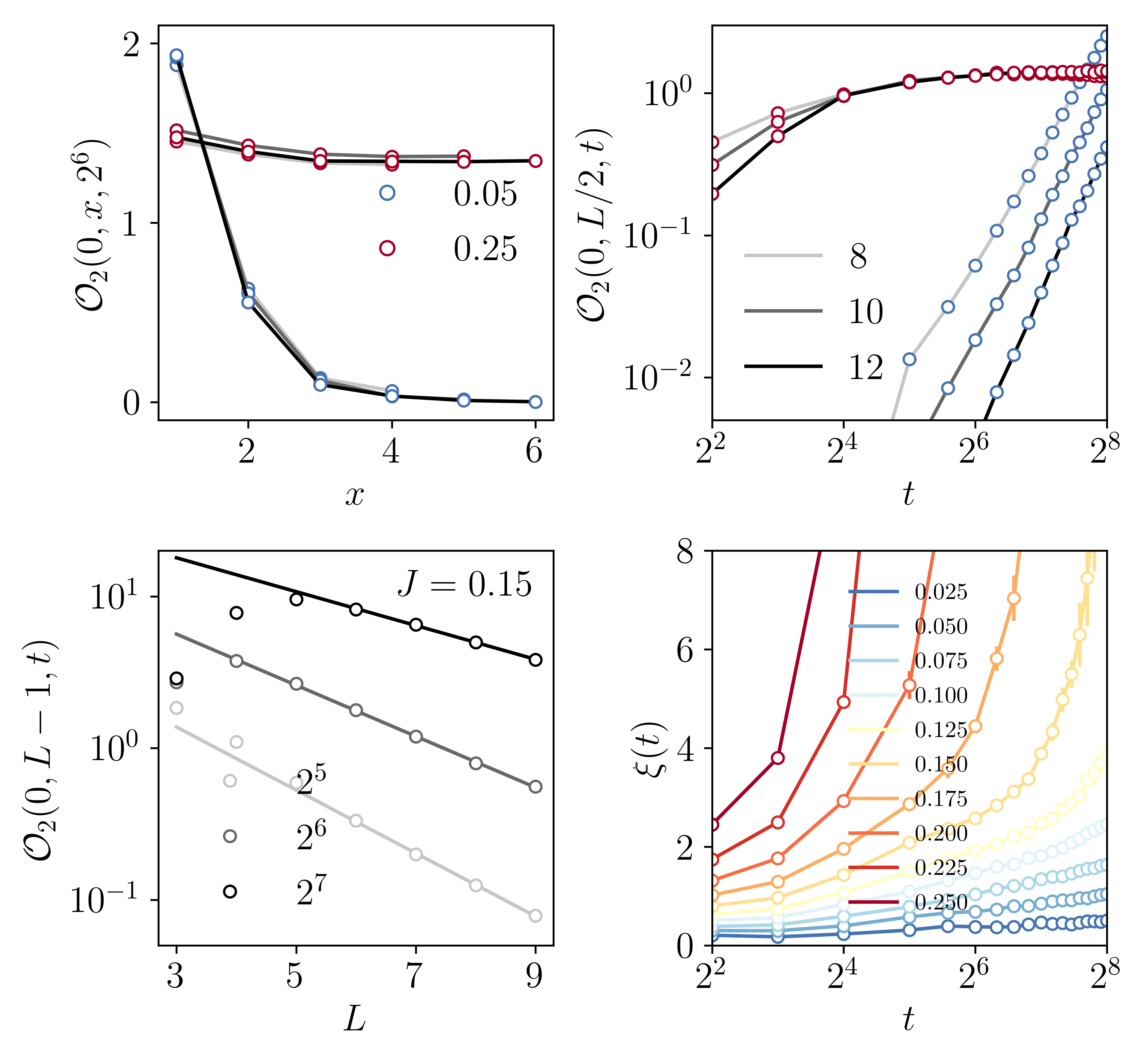
Hence $\xi(t)$ is small if the transfer matrix has a single dominant eigenvalue $\lambda(0,t)$, as in the MBL phase, and is divergent if $\lambda(0,t)$ and $\lambda(1,t)$ are degenerate at large $t$, as in the ergodic phase.

Alternatively, using the spectral decomposition of the Floquet operator, the two-point function can be expressed as sup

where $Z(x)$ is the Pauli matrix acting at site $x$, and $G_{mn}(t)=e^{i\theta_{n}t}\sum_{r=0}^{t-1}e^{i(2\pi/t+\theta_{m}-\theta_{n})r}$ selects for quasienergy separations $(\theta_{n}-\theta_{m})\sim 2\pi/t$. From this perspective, in the MBL phase we expect $\mathcal{O}_{2}(x,y,t)$ to be small for large $|x-y|$, because in that case there are few pairs of eigenstates $n$ and $m$ for which $\langle n|Z(x)|m\rangle$ and $\langle m|Z(y)|n\rangle$ are both large. Conversely, modelling these matrix elements using the eigenstate thermalisation hypothesis D’Alessio et al. 2016; Deutsch 2018; Deutsch 1991; Srednicki 1994; Rigol et al. 2008, expected to be applicable in the ergodic phase for $t\gg t_{\text{Th}}$, yields $\mathcal{O}_{2}(x,y,t)=1$ for $x\neq y$ and $t\ll t_{\text{H}}$ sup.

In Fig. 3 we test these suggestions for the behaviour of $\mathcal{O}_{2}(x,y,t)$ against numerics. From Fig. 3(a) we see a rapid decay with $|x-y|$ in the MBL phase ($J=0.05$), but find $\mathcal{O}_{2}(x,y,t)$ approximately independent of $|x-y|$ in the ergodic phase ($J=0.25$). Aspects of this behaviour depend on $t$, as we examine in Fig. 3(b). In the ergodic phase, variation is weak provided $t$ is sufficiently large. By contrast, in the MBL phase the amplitude of the two-point function increases with $t$ as a power law, and $\xi(t)$ increases slowly but remains small over the accessible range of $t$. We note that at low frequencies both power-law growth of matrix elements of local operators, and logarithmic growth in an associated lengthscale, are known features of the MBL phase Serbyn and Moore 2016; Gopalakrishnan et al. 2015; Serbyn et al. 2017; Crowley and Chandran 2021; Garratt et al. 2021. To investigate in detail the dependence of $\xi(t)$ on $t$, we extract it from the scaling of $\mathcal{O}_{2}(x,y,t)$ with separation sup, as illustrated in Fig. 3(c). Results for a range of $t$ and $J$ are shown in Fig. 3(d). These show a very rapid divergence of $\xi(t)$ with $t$ in the ergodic phase, and a much slower increase in the MBL phase.

The fact that $\xi(t)$ increases with $t$ for all values of $J$ raises the question of whether it is possible to make a sharp distinction between the two phases from the behaviour of $\mathcal{O}_{2}(x,y,t)$. This can be answered in the affirmative using the links between (i) $\xi(t)$ and $\lambda(\nu,t)$ [Eq. (10)], and (ii) $\lambda(\nu,t)$ and $\langle K(t)\rangle$ [Eq. (6)], together with the known behaviour of $\langle K(t)\rangle$ [Fig. 2]. These imply in the ergodic phase that $\xi(t)\gg L$ for $t_{\rm Th}\ll t<t_{\text{H}}$, since all $\lambda(\nu,t)$ are quasi-degenerate, and in the MBL phase that $\xi(t)\ll L$ for $t<t_{\text{H}}$, since $\lambda^{L}(0,t)\gg\lambda^{L}(\nu\neq 0,t)$. Hence, for large $L$ and $t$, $\mathcal{O}_{2}(x,y,t)$ reveals long-range order in the ergodic phase and disorder in the MBL phase. A prescription that ensures the two phases are distinguished is to take the limits $L,t\to\infty$ with $t=t_{\rm H}f\equiv 2^{L}f$ for fixed $0<f<1$.

In summary we have shown how, in a spatially extended many-body Floquet system with local interactions, the transition from an MBL phase to an ergodic one can be viewed as symmetry breaking. To do this we have related the disorder-averaged SFF to the spectrum of a transfer matrix acting in the space direction. In the ergodic phase this transfer matrix has $t$ leading eigenvalues which are asymptotically degenerate at large $t$, and these are associated with symmetry-breaking eigenvectors. The MBL phase on the other hand is characterised by a transfer matrix with one dominant eigenvalue, and the corresponding eigenvector breaks no symmetries. We have defined a local order parameter for the transition, and have shown that the behaviour of the SFF in the ergodic phase is associated with long-range correlations of this order parameter.

This perspective on the many-body localisation transition, and the set of tools we have developed, open new opportunities and raise a number of questions. While our focus here has been on behaviour deep within each phase, one can ask, for example, how $\xi(t)$ behaves in the vicinity of the critical point. Further questions concern the roles played by time-reversal symmetry, and by charge conservation. Finally, it would of course be interesting to adapt our ideas to a Hamiltonian system. This will require technical developments paralleling work described for Floquet systems in Ref. Garratt and Chalker 2021; a possible route might build on recent work described in Ref. Winer and Swingle 2020. Note that the broken symmetry in the Hamiltonian setting would be a continuous one.

In contrast with work emphasising rare-region effects at the transition De Roeck and Huveneers 2017; Agarwal et al. 2017, here we have focused only on an averaged quantity, the SFF. This nevertheless captures the distinction between the MBL and ergodic phases. A natural next step is to consider higher moments of the SFF, whereas an alternative is to study products of unaveraged transfer matrices, and the associated Lyapunov exponents Chan et al. 2021.

We are grateful to S. Roy for collaboration on related work, and to S. Parameswaran and A. Nahum for very useful discussions. This work was supported in part by EPSRC Grants EP/N01930X/1 and EP/S020527/1.

See pages 1 of suppmat_arxiv2.pdfSee pages 2 of suppmat_arxiv2.pdfSee pages 3 of suppmat_arxiv2.pdfSee pages 4 of suppmat_arxiv2.pdfSee pages 5 of suppmat_arxiv2.pdfSee pages 6 of suppmat_arxiv2.pdf

References

- Landau and Lifshitz (1980) L. D. Landau and E. M. Lifshitz, Statistical Physics (Pergamon Press, 1980).
- Sachdev (2011) S. Sachdev, Quantum Phase Transitions, 2nd ed. (Cambridge University Press, 2011).
- Altland and Simons (2010) A. Altland and B. D. Simons, Condensed matter field theory (Cambridge university press, 2010).
- Wegner (1979) F. Wegner, Z. Phys. B 35, 207 (1979).
- Fleishman and Anderson (1980) L. Fleishman and P. W. Anderson, Phys. Rev. B 21, 2366 (1980).
- Gornyi et al. (2005) I. V. Gornyi, A. D. Mirlin, and D. G. Polyakov, Phys. Rev. Lett. 95, 206603 (2005).
- Basko et al. (2006) D. Basko, I. Aleiner, and B. Altshuler, Ann. Phys. (N. Y.) 321, 1126 (2006).
- Oganesyan and Huse (2007) V. Oganesyan and D. A. Huse, Phys. Rev. B 75, 155111 (2007).
- Pal and Huse (2010) A. Pal and D. A. Huse, Phys. Rev. B 82, 174411 (2010).
- Nandkishore and Huse (2015) R. Nandkishore and D. A. Huse, Annu. Rev. Condens. Matter Phys. 6, 15 (2015).
- Abanin et al. (2019) D. A. Abanin, E. Altman, I. Bloch, and M. Serbyn, Rev. Mod. Phys. 91, 021001 (2019).
- D’Alessio et al. (2016) L. D’Alessio, Y. Kafri, A. Polkovnikov, and M. Rigol, Adv. Phys. 65, 239 (2016).
- Deutsch (2018) J. M. Deutsch, Rep. Prog. Phys. 81, 082001 (2018).
- Deutsch (1991) J. M. Deutsch, Phys. Rev. A 43, 2046 (1991).
- Srednicki (1994) M. Srednicki, Phys. Rev. E 50, 888 (1994).
- Rigol et al. (2008) M. Rigol, V. Dunjko, and M. Olshanii, Nature 452, 854 (2008).
- Nahum et al. (2017) A. Nahum, J. Ruhman, S. Vijay, and J. Haah, Phys. Rev. X 7, 031016 (2017).
- von Keyserlingk et al. (2018) C. W. von Keyserlingk, T. Rakovszky, F. Pollmann, and S. L. Sondhi, Phys. Rev. X 8, 021013 (2018).
- Nahum et al. (2018) A. Nahum, S. Vijay, and J. Haah, Phys. Rev. X 8, 021014 (2018).
- Li et al. (2018) Y. Li, X. Chen, and M. P. A. Fisher, Phys. Rev. B 98, 205136 (2018).
- Skinner et al. (2019) B. Skinner, J. Ruhman, and A. Nahum, Phys. Rev. X 9, 031009 (2019).
- Chan et al. (2019) A. Chan, R. M. Nandkishore, M. Pretko, and G. Smith, Phys. Rev. B 99, 224307 (2019).
- Li et al. (2019) Y. Li, X. Chen, and M. P. A. Fisher, Phys. Rev. B 100, 134306 (2019).
- Kos et al. (2018) P. Kos, M. Ljubotina, and T. Prosen, Phys. Rev. X 8, 021062 (2018).
- Chan et al. (2018a) A. Chan, A. De Luca, and J. T. Chalker, Phys. Rev. X 8, 041019 (2018a).
- Chan et al. (2018b) A. Chan, A. De Luca, and J. T. Chalker, Phys. Rev. Lett. 121, 060601 (2018b).
- Bertini et al. (2018) B. Bertini, P. Kos, and T. Prosen, Phys. Rev. Lett. 121, 264101 (2018).
- Garratt and Chalker (2021) S. J. Garratt and J. T. Chalker, Phys. Rev. X 11, 021051 (2021).
- Ponte et al. (2015) P. Ponte, Z. Papić, F. Huveneers, and D. A. Abanin, Phys. Rev. Lett. 114, 140401 (2015).
- Lazarides et al. (2015) A. Lazarides, A. Das, and R. Moessner, Phys. Rev. Lett. 115, 030402 (2015).
- Zhang et al. (2016) L. Zhang, V. Khemani, and D. A. Huse, Phys. Rev. B 94, 224202 (2016).
- Sünderhauf et al. (2018) C. Sünderhauf, D. Pérez-García, D. A. Huse, N. Schuch, and J. I. Cirac, Phys. Rev. B 98, 134204 (2018).
- Macé (2019) N. Macé, (2019), arXiv:1912.09489 .
- Akila et al. (2016) M. Akila, D. Waltner, B. Gutkin, and T. Guhr, J. Phys. A 49, 375101 (2016).
- Akila et al. (2017) M. Akila, D. Waltner, B. Gutkin, P. Braun, and T. Guhr, Phys. Rev. Lett. 118, 164101 (2017).
- Akila et al. (2018) M. Akila, B. Gutkin, P. Braun, D. Waltner, and T. Guhr, Ann. Phys. (N. Y.) 389, 250 (2018).
- Flack et al. (2020) A. Flack, B. Bertini, and T. Prosen, Phys. Rev. Research 2, 043403 (2020).
- Braun et al. (2020) P. Braun, D. Waltner, M. Akila, B. Gutkin, and T. Guhr, Phys. Rev. E 101, 052201 (2020).
- Bertini et al. (2019a) B. Bertini, P. Kos, and T. Prosen, Phys. Rev. X 9, 021033 (2019a).
- Piroli et al. (2020) L. Piroli, B. Bertini, J. I. Cirac, and T. Prosen, Phys. Rev. B 101, 094304 (2020).
- Lerose et al. (2021) A. Lerose, M. Sonner, and D. A. Abanin, Phys. Rev. X 11, 021040 (2021).
- Sonner et al. (2020) M. Sonner, A. Lerose, and D. A. Abanin, (2020), arXiv:2012.00777 .
- Claeys and Lamacraft (2021) P. W. Claeys and A. Lamacraft, Phys. Rev. Lett. 126, 100603 (2021).
- Bertini et al. (2019b) B. Bertini, P. Kos, and T. Prosen, Phys. Rev. Lett. 123, 210601 (2019b).
- (45) Supplemental material.
- Serbyn and Moore (2016) M. Serbyn and J. E. Moore, Phys. Rev. B 93, 041424 (2016).
- Gopalakrishnan et al. (2015) S. Gopalakrishnan, M. Müller, V. Khemani, M. Knap, E. Demler, and D. A. Huse, Phys. Rev. B 92, 104202 (2015).
- Serbyn et al. (2017) M. Serbyn, Z. Papić, and D. A. Abanin, Phys. Rev. B 96, 104201 (2017).
- Crowley and Chandran (2021) P. J. D. Crowley and A. Chandran, (2021), arXiv:2012.14393 .
- Garratt et al. (2021) S. J. Garratt, S. Roy, and J. T. Chalker, (2021), arXiv:2107.12387 .
- Winer and Swingle (2020) M. Winer and B. Swingle, (2020), arXiv:2012.01436 .
- De Roeck and Huveneers (2017) W. De Roeck and F. Huveneers, Phys. Rev. B 95, 155129 (2017).
- Agarwal et al. (2017) K. Agarwal, E. Altman, E. Demler, S. Gopalakrishnan, D. A. Huse, and M. Knap, Ann. Phys. (Berl.) 529, 1600326 (2017).
- Chan et al. (2021) A. Chan, A. De Luca, and J. T. Chalker, Phys. Rev. Research 3, 023118 (2021).