跳到论文正文
W Papers独立论文阅读器 arXiv:2012.11458 论文正文 计算阅读时间 · 0%
引用这篇论文根据当前论文元数据生成,正式投稿前建议核对。


License: arXiv.org perpetual non-exclusive license
arXiv:2012.11458v2 [math.CA] 08 Dec 2021

Decoupling for fractal subsets of the parabola

Alan Chang ACDepartment of Mathematics, Princeton University, Princeton, NJ 08544, USA Email address: alanchang@math.princeton.edu , Jaume de Dios Pont JDPDepartment of Mathematics, University of California Los Angeles, Portola Plaza 520, Los Angeles, CA 90095, USA Email address: jdedios@math.ucla.edu , Rachel Greenfeld RGDepartment of Mathematics, University of California Los Angeles, Portola Plaza 520, Los Angeles, CA 90095, USA Email address: greenfeld@math.ucla.edu , Asgar Jamneshan AJDepartment of Mathematics, Koç University, Rumelifeneri Yolu, 34450, Sariyer, Istanbul, Turkey Email address: ajamneshan@ku.edu.tr , Zane Kun Li ZKLDepartment of Mathematics, Indiana University Bloomington, Bloomington, IN-47405, USA Email address: zkli@iu.edu and José Madrid JMDepartment of Mathematics, University of California Los Angeles, Portola Plaza 520, Los Angeles, CA 90095, USA Email address: jmadrid@math.ucla.edu
Abstract.

We consider decoupling for a fractal subset of the parabola. We reduce studying l2​Lpl^{2}L^{p} decoupling for a fractal subset on the parabola {(t,t2):0≤t≤1}\{(t,t^{2}):0\leq t\leq 1\} to studying l2​Lp/3l^{2}L^{p/3} decoupling for the projection of this subset to the interval [0,1][0,1]. This generalizes the decoupling theorem of Bourgain-Demeter in the case of the parabola. Due to the sparsity and fractal like structure, this allows us to improve upon Bourgain-Demeter’s decoupling theorem for the parabola. In the case when p/3p/3 is an even integer we derive theoretical and computational tools to explicitly compute the associated decoupling constant for this projection to [0,1][0,1]. Our ideas are inspired by the recent work on ellipsephic sets by Biggs [1, 2] using nested efficient congruencing.

1. Introduction

Fix an integer q≥3q\geq 3, not necessarily a prime, and let δ⁡(i):=1/qi\delta(i):=1/q^{i}, i≥0i\geq 0. Let C0:=[0,1]C_{0}:=[0,1]. To construct level ii, we partition Ci−1C_{i-1} into intervals of length δ⁡(i)\delta(i), remove some of them, and denote by N⁡(i)N(i) the number of unremoved intervals. We associate C=⋂i≥0CiC=\bigcap_{i\geq 0}C_{i} with its levels CiC_{i}. For an interval II with |I|=δ⁡(i)|I|=\delta(i), δ⁡(i)>δ⁡(j)\delta(i)>\delta(j), Pδ⁡(j)​(I∩Cj)P_{\delta(j)}(I\cap C_{j}) will denote the collection of intervals that make up CjC_{j} which are contained in II. We also let Pδ⁡(i)​(Ci)=Pδ⁡(i)​([0,1]∩Ci)P_{\delta(i)}(C_{i})=P_{\delta(i)}([0,1]\cap C_{i}) be the collection of intervals of length δ⁡(i)\delta(i) that make up CiC_{i} and so N⁡(i)=#​Pδ⁡(i)​(Ci)N(i)=\#P_{\delta(i)}(C_{i}).

We call C=⋂i≥0CiC=\bigcap_{i\geq 0}C_{i} a generalized Cantor set and CiC_{i} a generalized Cantor set of level ii, when the following three conditions are satisfied:

  • •

    N⁡(i+j)=N⁡(i)​N​(j)N(i+j)=N(i)N(j).

  • •

    Ci⊂Ci−1C_{i}\subset C_{i-1}.

  • •

    The level CiC_{i} is similar to level Ci−1C_{i-1}. More precisely, for every interval I∈Pδ⁡(i−1)​(Ci−1)I\in P_{\delta(i-1)}(C_{i-1}), the set I∩CiI\cap C_{i} is a translate of q−1​Ci−1q^{-1}C_{i-1}.

By multiplicativity of N⁡(⋅)N(\cdot), given an I∈Pδ⁡(i)​(Ci)I\in P_{\delta(i)}(C_{i}) and i<ji<j, the number of intervals in Pδ⁡(j)​(Cj)P_{\delta(j)}(C_{j}) that are contained in II is N⁡(j−i)N(j-i). Additionally,

(1) δ(i)−dim(C)=N(i)\displaystyle\delta(i)^{-\dim(C)}=N(i)

where dim(C)\dim(C) is the Hausdorff dimension of CC. Note that in our definition, it is possible to let N⁡(i)=qiN(i)=q^{i} and so CiC_{i} is the partition of [0,1][0,1] into intervals of length 1/qi1/q^{i}.

The traditional middle-thirds Cantor set has q=3q=3 and N⁡(i)=2iN(i)=2^{i}. To avoid writing generalized Cantor set repeatedly, we will just call the above constructed set CC, a Cantor set and CiC_{i}, a level of Cantor set. A simple modification of our argument also allows it to work with asymmetric Cantor sets, however in order to simplify the arguments notation-wise, we do not pursue such a goal here.

Given a level of a Cantor set CiC_{i}, for each interval I∈Pδ⁡(i)​(Ci)I\in P_{\delta(i)}(C_{i}), let ℓI\ell_{I} denote the left endpoint of II and

ΩI:={ξ∈ℝ2:ℓI≤ξ1≤ℓI+δ(i),|ξ2−(2ℓI+δ(i))(ξ1−ℓI)−ℓI2|≤δ(i)2}.\displaystyle\Omega_{I}:=\{\xi\in\mathbb{R}^{2}:\ell_{I}\leq\xi_{1}\leq\ell_{I}+\delta(i),|\xi_{2}-(2\ell_{I}+\delta(i))(\xi_{1}-\ell_{I})-\ell_{I}^{2}|\leq\delta(i)^{2}\}.

Note that ΩI\Omega_{I} is a O⁡(δ⁡(i))×O⁡(δ​(i)2)O(\delta(i))\times O(\delta(i)^{2}) parallelogram that covers and is covered by a O⁡(δ​(i)2)O(\delta(i)^{2}) neighborhood of the piece of parabola above II.

For an interval II and f:ℝ→ℝf:\mathbb{R}\rightarrow\mathbb{R}, let fIf_{I} be defined such that fI^=f^​1I\widehat{f_{I}}=\widehat{f}1_{I}. Next for a region θ\theta and f:ℝ2→ℝf:\mathbb{R}^{2}\rightarrow\mathbb{R}, let fθf_{\theta} be defined such that fθ^=f^​1θ\widehat{f_{\theta}}=\widehat{f}1_{\theta}.

Finally, throughout this paper, for two nonnegative expressions XX and YY we use the notation X≲YX\lesssim Y or Y≳XY\gtrsim X to denote the bound X≤C​YX\leq CY for some absolute constant C>0C>0. If there are subscripts, for example, X≲pYX\lesssim_{p}Y, then we mean that there exists a constant Cp>0C_{p}>0 depending only on pp such that X≤Cp​YX\leq C_{p}Y. Additionally X∼YX\sim Y means that X≲YX\lesssim Y and Y≲XY\lesssim X.

1.1. Decoupling for CiC_{i} on the parabola

Fix a Cantor set CC and its levels CiC_{i}. For p≥2p\geq 2, let Dp​(δ​(i))D_{p}(\delta(i)) be the best constant such that

‖∑J∈Pδ⁡(i)​(Ci)fΩJ‖Lp​(ℝ2)≤Dp​(δ⁡(i))​(∑J∈Pδ⁡(i)​(Ci)‖fΩJ‖Lp​(ℝ2)2)1/2\displaystyle\|\sum_{J\in P_{\delta(i)}(C_{i})}f_{\Omega_{J}}\|_{L^{p}(\mathbb{R}^{2})}\leq D_{p}(\delta(i))(\sum_{J\in P_{\delta(i)}(C_{i})}\|f_{\Omega_{J}}\|_{L^{p}(\mathbb{R}^{2})}^{2})^{1/2}

for all Schwartz functions ff which are Fourier supported in ⋃J∈Pδ⁡(i)​(Ci)ΩJ\bigcup_{J\in P_{\delta(i)}(C_{i})}\Omega_{J}.

In the case when the Cantor set CC is the whole interval [0,1][0,1] and CiC_{i} is the partition of [0,1][0,1] into intervals of length δ⁡(i)\delta(i), we see that Dp​(δ​(i))D_{p}(\delta(i)) is just the regular l2​Lpl^{2}L^{p} decoupling constant for the parabola considered by Bourgain-Demeter in [4, 5] and so we immediately have Dp(δ(i))≲εδ(i)−ε(1+δ(i)−(12−3p))D_{p}(\delta(i))\lesssim_{\varepsilon}\delta(i)^{-\varepsilon}(1+\delta(i)^{-(\frac{1}{2}-\frac{3}{p})}). Our main result is the following generalization of Bourgain-Demeter’s parabola decoupling theorem.

Theorem 1.1.

Fix p≥2p\geq 2 and a Cantor set CC and its levels. Let κp​(C)\kappa_{p}(C) be the smallest number such that

(2) ∥∑J∈Pδ⁡(i)​(Ci)fJ∥Lp​(ℝ)≲p,ε,dim(C),N⁡(1)N(i)κp​(C)+ε(∑J∈Pδ⁡(i)​(Ci)∥fJ∥Lp​(ℝ)2)1/2\displaystyle\|\sum_{J\in P_{\delta(i)}(C_{i})}f_{J}\|_{L^{p}(\mathbb{R})}\lesssim_{p,\varepsilon,\dim(C),N(1)}N(i)^{\kappa_{p}(C)+\varepsilon}(\sum_{J\in P_{\delta(i)}(C_{i})}\|f_{J}\|_{L^{p}(\mathbb{R})}^{2})^{1/2}

for all Schwartz functions f:ℝ→ℝf:\mathbb{R}\rightarrow\mathbb{R} and all ii. Then the l2​L3​pl^{2}L^{3p} decoupling constant for CC is such that for every ε>0\varepsilon>0,

D3​p(δ(i))≲p,ε,dim(C),N⁡(1)N(i)κp​(C)+ε.D_{3p}(\delta(i))\lesssim_{p,\varepsilon,\dim(C),N(1)}N(i)^{\kappa_{p}(C)+\varepsilon}.

This theorem is proven in Section 2. The case of p=2p=2 is just an immediate application Bourgain-Demeter’s result on the parabola and (1). For p>2p>2, due to the sparsity and fractal structure of CC, we can do better than directly applying Bourgain-Demeter (see the examples summarized later or alternatively written in more detail in Section 3.3).

In the case when CC is the whole interval, Theorem 1.1 gives a sharp theorem for decoupling for the parabola. However, whether Theorem 1.1 is sharp for arbitrary Cantor sets CC is an area to be explored. Note that even if the ≲p,ε,dim(C),N⁡(1)\lesssim_{p,\varepsilon,\dim(C),N(1)} can be replaced with ≲p,ε\lesssim_{p,\varepsilon} (as is the case with our examples in Section 3.3), the proof of Theorem 1.1 adds in implicit constants that depends on dim(C)\dim(C) and N⁡(1)N(1).

The proof of Theorem 1.1 is inspired from [2], in particular one can think of [2, (1.2)] as an l2​L2​tl^{2}L^{2t} decoupling theorem on the line for which we then upgrade to an l2​L6​tl^{2}L^{6t} decoupling theorem on the parabola. However, Theorem 1.1 is more general than [2] since it is valid for arbitrary Cantor sets as defined on the first page rather than ellipsephic sets. Additionally, similar to the relation between [1] and [2], given a Cantor set CC and its levels, one can use ideas from [11] to write a version of Theorem 1.1 which upgrades l2​Lpl^{2}L^{p} decoupling on the line to l2​Lk⁡(k+1)​p/2l^{2}L^{k(k+1)p/2} decoupling on the moment curve ξ↦(ξ,ξ2,…,ξk)\xi\mapsto(\xi,\xi^{2},\ldots,\xi^{k}). However in this paper we only consider the case of the parabola.

Analogous to how [2] is related to Wooley’s nested efficient congruencing [20], the proof of Theorem 1.1 is similar in style to the proof of decoupling for the parabola found in [11, 16] though here we more closely follow Tao’s exposition [18] based off these two papers. For more discussion on decoupling interpretations of efficient congruencing, see [10, 11, 16] which are decoupling interpretations of the efficient congruencing papers [14], [20], and [17, Section 4.3], respectively.

Demeter in [7] generalized decoupling for the parabola in a different way. He considered the partition that arises from the set 𝒞α,n={0,α}+{0,α2}+⋯+{0,αn}\mathcal{C}_{\alpha,n}=\{0,\alpha\}+\{0,\alpha^{2}\}+\cdots+\{0,\alpha^{n}\} for 0≤α≤1/20\leq\alpha\leq 1/2 and proved l2​Lpl^{2}L^{p}, 2<p<62<p<6 decoupling estimates for the parabola decoupling question associated to this partition. The case α=1/2\alpha=1/2 corresponds to the uniform partition of [0,1][0,1] into intervals of length 2−n2^{-n}. More precisely, he showed that the decoupling constant is Oε​(2n​ε)O_{\varepsilon}(2^{n\varepsilon}) uniform in α\alpha. The difference between Demeter’s result and our work here is that he starts with the whole interval [0,1][0,1] and decouples into a self similar partition of [0,1][0,1] built from 𝒞α,n\mathcal{C}_{\alpha,n} while in our work we start with a sparse subset of [0,1][0,1] and decouple into its individual pieces. Additionally, the intervals in his partition have varying lengths while here our intervals all have the same length. See also [13] for a much stronger square function estimate for a lacunary partition of [0,1][0,1], the same comments on [7] also apply here.

1.2. Decoupling for CiC_{i} on [0,1][0,1]

Theorem 1.1 reduces studying D3​p​(δ​(i))D_{3p}(\delta(i)) to studying (2). We accomplish this in Section 3 for even integer pp and specific Cantor sets CC related to ellipsephic sets.

1.2.1. Discrete restriction and decoupling

First we define a discrete restriction for subsets S⊂ℤmS\subset\mathbb{Z}^{m} and decoupling constants for Ω⊂[0,1]\Omega\subset[0,1]. For S⊂ℤmS\subset\mathbb{Z}^{m}, let Ap,m​(S)A_{p,m}(S) be the best constant such that

‖∑ℓ∈Sa⁡(ℓ)​e​(ℓ⋅x)‖Lp​([0,1]m)≤Ap,m​(S)​(∑ℓ∈S|a⁡(ℓ)|2)1/2\displaystyle\|\sum_{\ell\in S}a(\ell)e(\ell\cdot x)\|_{L^{p}([0,1]^{m})}\leq A_{p,m}(S)(\sum_{\ell\in S}|a(\ell)|^{2})^{1/2}

for all a:S→ℝ≥0a:S\rightarrow\mathbb{R}_{\geq 0}. Next for a subset Ω⊂[0,1]\Omega\subset[0,1] partitioned into intervals II of equal length, let Kp​(Ω)K_{p}(\Omega) be the best constant such that

‖∑IfI‖Lp​(ℝ)≤Kp​(Ω)​(∑I‖fI‖Lp​(ℝ)2)1/2\displaystyle\|\sum_{I}f_{I}\|_{L^{p}(\mathbb{R})}\leq K_{p}(\Omega)(\sum_{I}\|f_{I}\|_{L^{p}(\mathbb{R})}^{2})^{1/2}

for all Schwartz functions f:ℝ→ℝf:\mathbb{R}\rightarrow\mathbb{R}.

Since we plan to discuss multiple different SS and SS will be related to Ω\Omega, we have chosen to emphasize the dependence of Ap,m​(S)A_{p,m}(S) and Kp​(Ω)K_{p}(\Omega) on SS and Ω\Omega rather than just the scale that comes naturally with Ω\Omega. This is different from what we did in the definition of Dp​(δ​(i))D_{p}(\delta(i)) above with CiC_{i} being associated naturally with the scale δ⁡(i)\delta(i).

1.2.2. Arithmetic Cantor sets and ellipsephic sets

We define an arithmetic Cantor set of base qq with digits 0≤d1<…<dk<q∈ℕ0\leq d_{1}<\ldots<d_{k}<q\in\mathbb{N} to be the set of fixed points of the iterated function system generated by the functions {fdj=(x↦q−1(x+dj))}j=1,…,k\left\{f_{d_{j}}=\left(x\mapsto q^{-1}(x+d_{j})\right)\right\}_{j=1,\dots,k}. This is a self-similar compact subset of [0,1][0,1] with Hausdorff dimension log⁡klog⁡q\frac{\log k}{\log q}. We will denote it by Cq{d1,…,dk}{C^{\{d_{1},\dots,d_{k}\}}_{q}}.

Denote by [Cq{d1,…,dk}]j[{C^{\{d_{1},\dots,d_{k}\}}_{q}}]_{j} the j−j-th level of Cq{d1,…,dk}{C^{\{d_{1},\dots,d_{k}\}}_{q}}, that is

[Cq{d1,…,dk}]j:=⋃(s1,…,sj)∈{d1,…,dk}j(fs1∘⋯∘fsj)​([0,1]).[{C^{\{d_{1},\dots,d_{k}\}}_{q}}]_{j}:=\bigcup_{(s_{1},\dots,s_{j})\in\{d_{1},\dots,d_{k}\}^{j}}(f_{s_{1}}\circ\dots\circ f_{s_{j}})([0,1]).

For brevity of notation, the intervals of length q−jq^{-j} in Pq−j​([Cq{d1,…,dk}]j)P_{q^{-j}}([{C^{\{d_{1},\dots,d_{k}\}}_{q}}]_{j}) will be denoted by [𝒞q{d1,…,dk}]j[{\mathscr{C}^{\{d_{1},\dots,d_{k}\}}_{q}}]_{j}. In particular, observe that

[𝒞q{d1,…,dk}]j={(fs1∘⋯∘fsj)​([0,1]):(s1,…,sj)∈{d1,…,dk}j}.[{\mathscr{C}^{\{d_{1},\dots,d_{k}\}}_{q}}]_{j}=\{(f_{s_{1}}\circ\dots\circ f_{s_{j}})([0,1]):(s_{1},\dots,s_{j})\in\{d_{1},\dots,d_{k}\}^{j}\}.

The standard middle thirds Cantor set is the arithmetic Cantor set C3{0,2}{C^{\{0,2\}}_{3}}. Note also that C3{0,1}{C^{\{0,1\}}_{3}} and C3{0,2}{C^{\{0,2\}}_{3}} are dilated copies of each other.

There is also a close connection between arithmetic Cantor sets and ellipsephic sets defined in [2]. An ellipsephic set of base qq with digits 0≤d1<⋯<dk<q∈ℕ0\leq d_{1}<\dots<d_{k}<q\in\mathbb{N} is the set of integers of the form ∑s=0j−1as​qs\sum_{s=0}^{j-1}a_{s}q^{s} (with as∈{d1,…,dk}a_{s}\in\{d_{1},\dots,d_{k}\}) for some j≥1j\geq 1. We will denote it by ℰq{d1,…,dk}{\mathcal{E}^{\{d_{1},\dots,d_{k}\}}_{q}}. We will use [ℰq{d1,…,dk}]j[{\mathcal{E}^{\{d_{1},\dots,d_{k}\}}_{q}}]_{j} to mean the set ℰq{d1,…,dk}∩[0,qj){\mathcal{E}^{\{d_{1},\dots,d_{k}\}}_{q}}\cap[0,q^{j}). Comparing the definitions of an arithmetic Cantor set and an ellipsephic set, we easily observe that

[Cq{d1,…,dk}]j=q−j​([ℰq{d1,…,dk}]j+[0,1]).[{C^{\{d_{1},\dots,d_{k}\}}_{q}}]_{j}=q^{-j}\left([{\mathcal{E}^{\{d_{1},\dots,d_{k}\}}_{q}}]_{j}+[0,1]\right).

Using the convenience that 2​n2n is even and expanding the L2​nL^{2n} norm (3.1), allows use to show 3.4

(3) K2​n​([𝒞q{d1,…,dk}]j)∼A2​n,1​([ℰq{d1,…,dk}]j)\displaystyle K_{2n}([{\mathscr{C}^{\{d_{1},\dots,d_{k}\}}_{q}}]_{j})\sim A_{2n,1}([{\mathcal{E}^{\{d_{1},\dots,d_{k}\}}_{q}}]_{j})

(where the implied constant is absolute) which connects decoupling and discrete restriction constants.

When we study A2​n,1​([ℰq{d1,…,dk}]j)A_{2n,1}([{\mathcal{E}^{\{d_{1},\dots,d_{k}\}}_{q}}]_{j}), we will say ℰq{d1,…,dk}{\mathcal{E}^{\{d_{1},\dots,d_{k}\}}_{q}} has no carryover if n​dk<qnd_{k}<q. In particular, this definition depends on the nn in question. Additionally note that we will say that ℰq{d1,…,dk}{\mathcal{E}^{\{d_{1},\dots,d_{k}\}}_{q}} has carryover if n​dk≥qnd_{k}\geq q. This terminology was inspired from the proof of [2, Lemma 2.2]. Using Freiman isomorphisms, we have the following nice proposition which simplifies greatly discrete restriction for ellipsephic sets when we have no carryover (see 3.5 for a more precise statement).

Proposition 1.2.

If ℰq{d1,…,dk}{\mathcal{E}^{\{d_{1},\dots,d_{k}\}}_{q}} is an ellipsephic set without carryover, then

A2​n,1​([ℰq{d1,…,dk}]j)=A2​n,1​([ℰq{d1,…,dk}]1)j.A_{2n,1}([{\mathcal{E}^{\{d_{1},\dots,d_{k}\}}_{q}}]_{j})=A_{2n,1}([{\mathcal{E}^{\{d_{1},\dots,d_{k}\}}_{q}}]_{1})^{j}.
Remark 1.

Łaba and Wang in [15] consider a restriction estimate for a certain kind of fractal measure in ℝd\mathbb{R}^{d}. The main ingredient in the proof of their main theorem is a decoupling estimate for a particular type of Cantor set on the line built out of a Λ⁡(p)\Lambda(p)-set (see Lemma 5, Section 4, and Proposition 1 of [15] for more details, see also [3] for the existence of Λ⁡(p)\Lambda(p) sets). The techniques by which they upgrade a Λ⁡(p)\Lambda(p) set to a Cantor set multiscale decoupling theorem on the line can probably also be applied in our case, though here the point of view we take is more algebraic and is closer in spirit to the number theoretic side of things.

1.3. Examples

As an illustration of the the tools developed above we can consider the case when n=2n=2 and then very explicitly study A4,1​([ℰq{d1,…,dk}]j)A_{4,1}([{\mathcal{E}^{\{d_{1},\dots,d_{k}\}}_{q}}]_{j}) as 3.1 turns such study into an optimization problem subject to a quadratic constraint which we can very explicitly compute. This combined with (3) allows us to upgrade l2​L4l^{2}L^{4} discrete restriction for an ellipsephic set to l2​L4l^{2}L^{4} decoupling for an arithmetic Cantor set. In particular, below is a summary of Examples 1-5 we derived in Section 3.3.

CiC_{i} δ⁡(i)\delta(i) N⁡(i)N(i) K4​(Ci)K_{4}(C_{i})
[Cq{0,1}]i,q>2[C_{q}^{\{0,1\}}]_{i},q>2 q−iq^{-i} 2i2^{i} ∼(2i)14​log2​(3/2)\sim(2^{i})^{\frac{1}{4}\log_{2}(3/2)}
[C3{0,2}]i[C_{3}^{\{0,2\}}]_{i} 3−i3^{-i} 2i2^{i} ∼(2i)14​log2​(3/2)\sim(2^{i})^{\frac{1}{4}\log_{2}(3/2)}
[Cq{0,1,2}]i,q>4[C_{q}^{\{0,1,2\}}]_{i},q>4 q−iq^{-i} 3i3^{i} ∼(3i)14​log3​(15/7)\sim(3^{i})^{\frac{1}{4}\log_{3}(15/7)}
[Cq{0,1,3}]i,q>6[C_{q}^{\{0,1,3\}}]_{i},q>6 q−iq^{-i} 3i3^{i} ∼(3i)14​log3​(5/3)\sim(3^{i})^{\frac{1}{4}\log_{3}(5/3)}
[Cq{02,12,…,⌊q⌋2}]i,q≥exp⁡(exp⁡(O⁡(1ε)))[C_{q}^{\{0^{2},1^{2},\ldots,\lfloor\sqrt{q}\rfloor^{2}\}}]_{i},q\geq\exp(\exp(O(\frac{1}{\varepsilon}))) q−iq^{-i} (⌊q⌋+1)i(\lfloor\sqrt{q}\rfloor+1)^{i} ≲εN(i)ε\lesssim_{\varepsilon}N(i)^{\varepsilon}

Note that from the proof of these examples in Section 3.3, the implied constants do not depend on dim(C)\dim(C) or N⁡(1)N(1). We only studied the n=2n=2 case out for convenience to demonstrate our methods but it is not a serious constraint.

Remark 2.

The ellipsephic set associated to the Cantor set in the last row of the table above was considered by Biggs in [2, Corollary 1.4]. The result in that row should be read as follows: Fix an arbitrary ε>0\varepsilon>0. Choose an integer q≥exp⁡(exp⁡(O⁡(1/ε)))q\geq\exp(\exp(O(1/\varepsilon))) and consider [Cq{02,12,…,⌊q⌋2}]i[C_{q}^{\{0^{2},1^{2},\ldots,\lfloor\sqrt{q}\rfloor^{2}\}}]_{i}. Note that here the Cantor set depends on qq and so also ε\varepsilon. Then we showed that the l2​L4l^{2}L^{4} decoupling constant for level ii of this Cantor set is ≲εN(i)ε\lesssim_{\varepsilon}N(i)^{\varepsilon} where N⁡(i)=(⌊q⌋+1)iN(i)=(\lfloor q\rfloor+1)^{i}.

Remark 3.

The example in the second row of the table above is associated to the ellipsephic set [ℰ3{0,2}]j[\mathcal{E}_{3}^{\{0,2\}}]_{j} which does have carryover. However, the map x↦x/2x\mapsto x/2 is a Freiman isomorphism between [ℰ3{0,2}]j[\mathcal{E}_{3}^{\{0,2\}}]_{j} and [ℰ3{0,1}]j[\mathcal{E}_{3}^{\{0,1\}}]_{j} and the latter ellipsephic set does not have carryover. Since Freiman isomorphisms do not change numerology (see the equality case of (25)), the numerology of the second row is the same as that of the first row.

Remark 4.

Note that Cq{0,1,2}C_{q}^{\{0,1,2\}} and Cq{0,1,3}C_{q}^{\{0,1,3\}} for q>6q>6 have the same Hausdorff dimension but their associated l2​L4l^{2}L^{4} decoupling constants are different. In 3.6 we show that given a Hausdorff dimension d=logs⁡rd=\log_{s}r with 0<d<10<d<1 and r,s∈ℕr,s\in\mathbb{N}, there exists an arithmetic Cantor set CC such that the associated decoupling exponent κ2​n​(C)\kappa_{2n}(C) as defined in (2) is as large as possible. This means that for arbitrary arithmetic Cantor sets K2​n​(C)K_{2n}(C) does not just depend on the Cantor set, but rather also on arithmetic properties of the set.

Remark 5.

A careful look at the proof of Example 3 (the third row in the table above) shows curiously that the optimizer of discrete restriction for [ℰq{0,1,2}]1[\mathcal{E}_{q}^{\{0,1,2\}}]_{1}, q>4q>4 (and hence also [ℰq{0,1,2}]j[\mathcal{E}_{q}^{\{0,1,2\}}]_{j} by 3.5 because of lack of carryover). This is different from the other examples in Section 3.3 and the observation that the choice of a:{1,…,ℕ}→ℝ≥0a:\{1,\ldots,\mathbb{N}\}\rightarrow\mathbb{R}_{\geq 0} being the constant function below witnesses the case of equality of the estimates

‖∑1≤ℓ≤Na⁡(ℓ)​e​(ℓ​x)‖L2​n​([0,1])≤N12−1n​(∑1≤ℓ≤N|a⁡(ℓ)|2)1/2\|\sum_{1\leq\ell\leq N}a(\ell)e(\ell x)\|_{L^{2n}([0,1])}\leq N^{\frac{1}{2}-\frac{1}{n}}(\sum_{1\leq\ell\leq N}|a(\ell)|^{2})^{1/2}

and

∥∑1≤n≤Na(n)e(nx+n2t)∥L6​([0,1]2)≲εNε(∑1≤n≤N|a(n)|2)1/2\|\sum_{1\leq n\leq N}a(n)e(nx+n^{2}t)\|_{L^{6}([0,1]^{2})}\lesssim_{\varepsilon}N^{\varepsilon}(\sum_{1\leq n\leq N}|a(n)|^{2})^{1/2}

for all {a⁡(n)}∈ℓ2​(ℕ)\{a(n)\}\in\ell^{2}(\mathbb{N}). This example suggests potential differences between discrete restriction and solution counting problems in certain cases.

In the table below we feed our results into Theorem 1.1. Each row should be compared to the estimate that D12(δ(i))≲εδ(i)−1/4−εD_{12}(\delta(i))\lesssim_{\varepsilon}\delta(i)^{-1/4-\varepsilon} obtained from a direct application of Bourgain-Demeter’s decoupling theorem for the parabola.

CiC_{i} δ⁡(i)\delta(i) N⁡(i)N(i) Applying Theorem 1.1
[Cq{0,1}]i,q>2[C_{q}^{\{0,1\}}]_{i},q>2 q−iq^{-i} 2i2^{i} D12(δ(i))≲ε,dim(C)(2i)14​log2⁡(3/2)+εD_{12}(\delta(i))\lesssim_{\varepsilon,\dim(C)}(2^{i})^{\frac{1}{4}\log_{2}(3/2)+\varepsilon}
[C3{0,2}]i[C_{3}^{\{0,2\}}]_{i} 3−i3^{-i} 2i2^{i} D12(δ(i))≲ε(2i)14​log2⁡(3/2)+εD_{12}(\delta(i))\lesssim_{\varepsilon}(2^{i})^{\frac{1}{4}\log_{2}(3/2)+\varepsilon}
[Cq{0,1,2}]i,q>4[C_{q}^{\{0,1,2\}}]_{i},q>4 q−iq^{-i} 3i3^{i} D12(δ(i))≲ε,dim(C)(3i)14​log3⁡(15/7)+εD_{12}(\delta(i))\lesssim_{\varepsilon,\dim(C)}(3^{i})^{\frac{1}{4}\log_{3}(15/7)+\varepsilon}
[Cq{0,1,3}]i,q>6[C_{q}^{\{0,1,3\}}]_{i},q>6 q−iq^{-i} 3i3^{i} D12(δ(i))≲ε,dim(C)(3i)14​log3⁡(5/3)+εD_{12}(\delta(i))\lesssim_{\varepsilon,\dim(C)}(3^{i})^{\frac{1}{4}\log_{3}(5/3)+\varepsilon}
[Cq{02,12,…,⌊q⌋2}]i,q≥exp⁡(exp⁡(O⁡(1ε)))[C_{q}^{\{0^{2},1^{2},\ldots,\lfloor\sqrt{q}\rfloor^{2}\}}]_{i},q\geq\exp(\exp(O(\frac{1}{\varepsilon}))) q−iq^{-i} (⌊q⌋+1)i(\lfloor\sqrt{q}\rfloor+1)^{i} D12(δ(i))≲ε,N⁡(1)N(i)εD_{12}(\delta(i))\lesssim_{\varepsilon,N(1)}N(i)^{\varepsilon}

Note that in the first four rows we have N⁡(1)∼1N(1)\sim 1 while in the second and last row we have dim(C)∼1\dim(C)\sim 1. Whether our estimates for D12​(δ​(i))D_{12}(\delta(i)) above are sharp remain an area to be explored (in other words, for example, is there an ff Fourier supported in ⋃J∈[𝒞3{0,2}]iΩJ\bigcup_{J\in[\mathscr{C}_{3}^{\{0,2\}}]_{i}}\Omega_{J} such that D12​(δ⁡(i))≳(2i)14​log2​(3/2)D_{12}(\delta(i))\gtrsim(2^{i})^{\frac{1}{4}\log_{2}(3/2)}). Continuing the discussion in Remark 2, the last row in the table above should be compared to [2, Corollary 1.4].

Finally the above methods are very efficient in studying the case when the ellipsephic set does not have carryover and some cases with carryover but which are Freiman isomorphic to a case which has no carryover. To study the case when the ellipsehic set has carryover we develop an approximation (3.7) which allows us to numerically approximate the l2​L2​nl^{2}L^{2n} decoupling constant on [0,1][0,1] for a given arithmetic Cantor set (see Section 3.4 for more details).

1.4. Application to solution counting

We end with some applications of our estimates to number theory, in particular to solution counting in Vinogradov systems.

1.4.1. The Cantor set C3{0,1}C_{3}^{\{0,1\}}

Consider [C3{0,1}]j[C_{3}^{\{0,1\}}]_{j} and the associated ellipsephic set [ℰ3{0,1}]j[\mathcal{E}_{3}^{\{0,1\}}]_{j}. Note #​[ℰ3{0,1}]j∼2i\#[\mathcal{E}_{3}^{\{0,1\}}]_{j}\sim 2^{i}. We first obtained that K4​([C3{0,1}]j)∼A4​([ℰ3{0,1}]j)∼(3/2)j/4K_{4}([C_{3}^{\{0,1\}}]_{j})\sim A_{4}([\mathcal{E}_{3}^{\{0,1\}}]_{j})\sim(3/2)^{j/4}. This immediately implies that the number of 4-tuples to

x1+x2=x3+x4x_{1}+x_{2}=x_{3}+x_{4}

with 1≤xi≤3j1\leq x_{i}\leq 3^{j} and xi∈[ℰ3{0,1}]jx_{i}\in[\mathcal{E}_{3}^{\{0,1\}}]_{j} is (3/2)j​22​j=6j(3/2)^{j}2^{2j}=6^{j}. This should be compared to solving x1+x2=x3+x4x_{1}+x_{2}=x_{3}+x_{4} where 1≤xi≤2j1\leq x_{i}\leq 2^{j} which would give 8j8^{j} such 4-tuples. The 6 in 6j6^{j} can be explained by the fact that since ℰ3{0,1}\mathcal{E}_{3}^{\{0,1\}} in this case has no carryover (2⋅1<32\cdot 1<3), we can look one digit at a time and there are 6 solutions to a+b=c+da+b=c+d where a,b,c,d∈{0,1}a,b,c,d\in\{0,1\}.

Next we obtained that D12(δ(j))≲ε(3/2)j/4+εD_{12}(\delta(j))\lesssim_{\varepsilon}(3/2)^{j/4+\varepsilon} where δ⁡(j)=3−j\delta(j)=3^{-j}. Using the standard reduction from decoupling estimates to solving Vinogradov [6] we see that the number of solutions to the system

(4) x1+x2+⋯+x6\displaystyle x_{1}+x_{2}+\cdots+x_{6} =y1+y2+⋯+y6\displaystyle=y_{1}+y_{2}+\cdots+y_{6}
x12+x22+⋯+x62\displaystyle x_{1}^{2}+x_{2}^{2}+\cdots+x_{6}^{2} =y12+y22+⋯+y62\displaystyle=y_{1}^{2}+y_{2}^{2}+\cdots+y_{6}^{2}

where 1≤xi,yi≤3j1\leq x_{i},y_{i}\leq 3^{j} and xi,yi∈[ℰ3{0,1}]jx_{i},y_{i}\in[\mathcal{E}_{3}^{\{0,1\}}]_{j} is ≲ε(32)3​j+ε26​j=63​j+O⁡(ε)\lesssim_{\varepsilon}(\frac{3}{2})^{3j+\varepsilon}2^{6j}=6^{3j+O(\varepsilon)}. This should be compared to the lower bound of O⁡(26​j)O(2^{6j}) coming from the diagonal solutions.

1.4.2. The Cantor set Cq{02,12,…,⌊q⌋2}C_{q}^{\{0^{2},1^{2},\ldots,\lfloor\sqrt{q}\rfloor^{2}\}}

Fix arbitrary ε>0\varepsilon>0. Choose qq an integer (not necessarily prime) such that q≥exp⁡(exp⁡(O⁡(1/ε)))q\geq\exp(\exp(O(1/\varepsilon))) and consider the ellipsephic set [ℰq{02,12,…,⌊q⌋2}]j[\mathcal{E}_{q}^{\{0^{2},1^{2},\ldots,\lfloor\sqrt{q}\rfloor^{2}\}}]_{j} associated to the Cantor set [Cq{02,12,…,⌊q⌋2}]j[C_{q}^{\{0^{2},1^{2},\ldots,\lfloor\sqrt{q}\rfloor^{2}\}}]_{j}. Then the estimate that D12(δ(j))≲ε,N⁡(1)N(j)εD_{12}(\delta(j))\lesssim_{\varepsilon,N(1)}N(j)^{\varepsilon} implies that the number of solutions to the system (4) where 1≤xi,yi≤qj1\leq x_{i},y_{i}\leq q^{j} and xi,yi∈[ℰq{02,12,…,⌊q⌋2}]jx_{i},y_{i}\in[\mathcal{E}_{q}^{\{0^{2},1^{2},\ldots,\lfloor\sqrt{q}\rfloor^{2}\}}]_{j} is ≲ε,N⁡(1)N(j)6+ε\lesssim_{\varepsilon,N(1)}N(j)^{6+\varepsilon}. This rederives the implication obtained in [2, Corollary 1.4] (where our N⁡(j)N(j) is her YY).

Remark 6.

In the system considered in Section 1.4.1, our upper bound is quite large compared to the lower bound of 26​N2^{6N} which come from the diagonal contribution. In the following, we argue that given an ellipsephic set (whose associated Cantor set has dimension dd), then when the number of variables is sufficiently large depending on dd, then the contribution of the non-diagonal solutions will be greater than that of the diagonal solutions.

More precisely, fix an arbitrary arithmetic Cantor set Cq{d1,…,dk}C_{q}^{\{d_{1},\ldots,d_{k}\}} with Hausdorff dimension d∈(0,1)d\in(0,1) and consider the associated ellipsephic set ℰX:=[ℰq{d1,…,dk}]j\mathcal{E}_{X}:=[\mathcal{E}_{q}^{\{d_{1},\ldots,d_{k}\}}]_{j} where we have written X=qjX=q^{j}. Then #​ℰX∼Xd\#\mathcal{E}_{X}\sim X^{d}. We consider the question of how many solutions are there to the system

(5) x1+x2+⋯+xs\displaystyle x_{1}+x_{2}+\cdots+x_{s} =xs+1+xs+2+⋯+x2​s\displaystyle=x_{s+1}+x_{s+2}+\cdots+x_{2s}
x12+x22+⋯+xs2\displaystyle x_{1}^{2}+x_{2}^{2}+\cdots+x_{s}^{2} =xs+12+xs+22+⋯+x2​s2\displaystyle=x_{s+1}^{2}+x_{s+2}^{2}+\cdots+x_{2s}^{2}

where xi∈ℰXx_{i}\in\mathcal{E}_{X}. The contribution from the diagonal solutions is O⁡(Xs​d)O(X^{sd}). We claim that for sufficiently large ss there will always be more than O⁡(Xs​d)O(X^{sd}) many solutions.

Consider the map

Σ:(ℰX)s\displaystyle\Sigma:(\mathcal{E}_{X})^{s} ⟶[−s​X,s​X]×[−s​X2,s​X2]\displaystyle\longrightarrow[-sX,sX]\times[-sX^{2},sX^{2}]
(a1,a2,…,as)\displaystyle(a_{1},a_{2},\ldots,a_{s}) ⟼(a1+⋯+as,a12+⋯+as2)\displaystyle\longmapsto(a_{1}+\cdots+a_{s},a_{1}^{2}+\cdots+a_{s}^{2})

The map Σ\Sigma goes from a set of cardinality O⁡(Xs​d)O(X^{sd}) to a set of cardinality O⁡(s2​X3)O(s^{2}X^{3}). For notational convenience let AX=[−s​X,s​X]×[−s​X2,s​X2]A_{X}=[-sX,sX]\times[-sX^{2},sX^{2}]. The number of solutions Js​(X)J_{s}(X) to (5) is bounded below by:

Js​(X)=\displaystyle J_{s}(X)= ∑(n1,n2)∈AX(∑a1j+⋯+asj=njai∈(ℰX)s,j=1,21)2\displaystyle\sum_{(n_{1},n_{2})\in A_{X}}(\sum_{\begin{subarray}{c}a_{1}^{j}+\dots+a_{s}^{j}=n_{j}\\ a_{i}\in(\mathcal{E}_{X})^{s},j=1,2\end{subarray}}1)^{2}
≥\displaystyle\geq |AX|−1​(∑(n1,n2)∈AX∑a1j+⋯+asj=njai∈(ℰX)s,j=1,21)2\displaystyle|A_{X}|^{-1}(\sum_{(n_{1},n_{2})\in A_{X}}\sum_{\begin{subarray}{c}a_{1}^{j}+\dots+a_{s}^{j}=n_{j}\\ a_{i}\in(\mathcal{E}_{X})^{s},j=1,2\end{subarray}}1)^{2}
=\displaystyle= (O⁡(s2​X3))−1⋅(O⁡(Xs​d))2=O⁡(X2​s​d−3/s2)\displaystyle(O(s^{2}X^{3}))^{-1}\cdot(O(X^{sd}))^{2}=O(X^{2sd-3}/s^{2})

Therefore the number of solutions to (5) is at least O⁡(X2​s​d−3/s2)O(X^{2sd-3}/s^{2}). Comparing this to the number of diagonal solutions O⁡(Xs​d)O(X^{sd}) shows that for ss sufficiently large (depending on Hausdorff dimension), the contribution of the off-diagonal solutions are more than the diagonal solutions.

Acknowledgements

JD was partially supported by “La Caixa” Fellowship LCF/ BQ/ AA17/ 11610013. RG was partially supported by the Eric and Wendy Schmidt Postdoctoral Award. AJ was supported by DFG-research fellowship JA 2512/3-1. ZL is supported by NSF grant DMS-1902763. ZL is also grateful to the Department of Mathematics at the University of Chicago and the University of California, Los Angeles for their hospitality when he visited in February 2020.

The authors would also like to thank Iqra Altaf, Kirsti Biggs, Julia Brandes, Ciprian Demeter, Bingyang Hu, and Terence Tao for helpful comments, discussions, and suggestions.

2. Proof of Theorem 1.1

Fix a Cantor set CC (and its levels). Much like the proof of decoupling for the parabola in [16], the proof of 1.1 reduces to four lemmas: parabolic rescaling, bilinear reduction, the key estimate, and Hölder’s inequality.

2.1. Parabolic rescaling and bilinear reduction

We first start with the parabolic rescaling lemma. The proof is fairly standard, but we include it here for convenience.

Lemma 2.1 (Parabolic rescaling).

Suppose 0≤δ⁡(j)≤δ⁡(i)≤10\leq\delta(j)\leq\delta(i)\leq 1 and I∈Pδ⁡(i)​(Ci)I\in P_{\delta(i)}(C_{i}). Then

(6) ‖∑J∈Pδ⁡(j)​(I∩Cj)fΩJ‖Lp​(ℝ2)≤Dp​(δ⁡(j−i))​(∑J∈Pδ⁡(j)​(I∩Cj)‖fΩJ‖Lp​(ℝ2)2)1/2.\displaystyle\|\sum_{J\in P_{\delta(j)}(I\cap C_{j})}f_{\Omega_{J}}\|_{L^{p}(\mathbb{R}^{2})}\leq D_{p}(\delta(j-i))\left(\sum_{J\in P_{\delta(j)}(I\cap C_{j})}\|f_{\Omega_{J}}\|_{L^{p}(\mathbb{R}^{2})}^{2}\right)^{1/2}.
Proof.

Write I=[a,a+δ⁡(i)]I=[a,a+\delta(i)]. Consider the “Galilean transform” SI:ℝ2→ℝ2S_{I}:\mathbb{R}^{2}\to\mathbb{R}^{2} represented by the matrix

(δ​(i)−100δ​(i)−2)​(10−2​a1).\displaystyle\begin{pmatrix}\delta(i)^{-1}&0\\ 0&\delta(i)^{-2}\end{pmatrix}\begin{pmatrix}1&0\\ -2a&1\end{pmatrix}.

The key geometric observation is that since CiC_{i} is a level of a Cantor set (and Cantor set levels are similar), we have a bijection Pδ⁡(j)​(I∩Cj)→Pδ⁡(j−i)​(Cj−i)P_{\delta(j)}(I\cap C_{j})\to P_{\delta(j-i)}(C_{j-i}) given by J↦J′=δ​(i)−1​(J−a)J\mapsto J^{\prime}=\delta(i)^{-1}(J-a), and furthermore,

(7) SI​(ΩJ−(a,a2))=ΩJ′.\displaystyle S_{I}(\Omega_{J}-(a,a^{2}))=\Omega_{J^{\prime}}.

Define gI(y):=f(SI⊤y)e(−SI(a,a2)⋅y)g_{I}(y):=f(S_{I}^{\top}y)e(-S_{I}(a,a^{2})\cdot y), so that gI^​(η)=δ​(i)3​f^​(SI−1​η+(a,a2))\widehat{g_{I}}(\eta)=\delta(i)^{3}\widehat{f}(S_{I}^{-1}\eta+(a,a^{2})). With J,J′J,J^{\prime} as above, we have

fΩJ​(x)\displaystyle f_{\Omega_{J}}(x) =∫ΩJf^​(ξ)​e​(ξ⋅x)​𝑑ξ\displaystyle=\int_{\Omega_{J}}\widehat{f}(\xi)e(\xi\cdot x)\,d\xi
=e⁡(x⋅(a,a2))​∫ΩJ′gI^​(η)​e​(η⋅(SI−1)⊤​x)​𝑑η=e⁡(x⋅(a,a2))​(gI)ΩJ′​((SI−1)⊤​x)\displaystyle=e(x\cdot(a,a^{2}))\int_{\Omega_{J^{\prime}}}\widehat{g_{I}}(\eta)e(\eta\cdot(S_{I}^{-1})^{\top}x)\,d\eta=e(x\cdot(a,a^{2}))(g_{I})_{\Omega_{J^{\prime}}}((S_{I}^{-1})^{\top}x)

where in the second equality we made the change of variables η=SI​(ξ−(a,a2))\eta=S_{I}(\xi-(a,a^{2})) and used (7). Therefore,

|∑J∈Pδ⁡(j)​(I∩Cj)fΩJ​(x)|=|∑J′∈Pδ⁡(j−i)​(Cj−i)(gI)ΩJ′​((SI−1)⊤​x)|\displaystyle|\sum_{J\in P_{\delta(j)}(I\cap C_{j})}f_{\Omega_{J}}(x)|=|\sum_{J^{\prime}\in P_{\delta(j-i)}(C_{j-i})}(g_{I})_{\Omega_{J^{\prime}}}((S_{I}^{-1})^{\top}x)|

and hence

‖∑J∈Pδ⁡(j)​(I∩Cj)fΩJ‖Lp​(ℝ2)\displaystyle\|\sum_{J\in P_{\delta(j)}(I\cap C_{j})}f_{\Omega_{J}}\|_{L^{p}(\mathbb{R}^{2})} =δ(i)−3/p∥∑J′∈Pδ⁡(j−i)​(Cj−i)(gI)ΩJ′∥Lp​(ℝ2)\displaystyle=\delta(i)^{-3/p}\|\sum_{J^{\prime}\in P_{\delta(j-i)}(C_{j-i})}(g_{I})_{\Omega_{J^{\prime}}}\|_{L^{p}(\mathbb{R}^{2})}
≤δ(i)−3/pDp(δ(j−i))(∑J′∈Pδ⁡(j−i)​(Cj−i)∥(gI)ΩJ′∥Lp​(ℝ2)2)1/2.\displaystyle\leq\delta(i)^{-3/p}D_{p}(\delta(j-i))(\sum_{J^{\prime}\in P_{\delta(j-i)}(C_{j-i})}\|(g_{I})_{\Omega_{J^{\prime}}}\|_{L^{p}(\mathbb{R}^{2})}^{2})^{1/2}.

Reversing all the change of variables then obtains the right hand side of (6). ∎

Parabolic rescaling implies the following immediate corollary.

Corollary 2.2 (Almost multiplicativity).

We have

Dp​(δ⁡(i+j))≤Dp​(δ⁡(i))​Dp​(δ⁡(j)).D_{p}(\delta(i+j))\leq D_{p}(\delta(i))D_{p}(\delta(j)).

Next we define the following bilinear constant. Let 0≤δ⁡(j)≤δ⁡(i1),δ⁡(i2)≤δ⁡(k)≤10\leq\delta(j)\leq\delta(i_{1}),\delta(i_{2})\leq\delta(k)\leq 1. Let Mp​(j,k,i1,i2)M_{p}(j,k,i_{1},i_{2}) to be the best constant such that one has the estimate

∫ℝ2\displaystyle\int_{\mathbb{R}^{2}} |∑J1∈Pδ⁡(j)​(I1∩Cj)fΩJ1|p​|∑J2∈Pδ⁡(j)​(I2∩Cj)gΩJ2|2​p\displaystyle|\sum_{J_{1}\in P_{\delta(j)}(I_{1}\cap C_{j})}f_{\Omega_{J_{1}}}|^{p}|\sum_{J_{2}\in P_{\delta(j)}(I_{2}\cap C_{j})}g_{\Omega_{J_{2}}}|^{2p}
≤Mp​(j,k,i1,i2)3​p​(∑J1∈Pδ⁡(j)​(I1∩Cj)‖fΩJ1‖L3​p​(ℝ2)2)p/2​(∑J2∈Pδ⁡(j)​(I2∩Cj)‖gΩJ2‖L3​p​(ℝ2)2)p\displaystyle\leq M_{p}(j,k,i_{1},i_{2})^{3p}(\sum_{J_{1}\in P_{\delta(j)}(I_{1}\cap C_{j})}\|f_{\Omega_{J_{1}}}\|_{L^{3p}(\mathbb{R}^{2})}^{2})^{p/2}(\sum_{J_{2}\in P_{\delta(j)}(I_{2}\cap C_{j})}\|g_{\Omega_{J_{2}}}\|_{L^{3p}(\mathbb{R}^{2})}^{2})^{p}

for all I1∈Pδ⁡(i1)​(Ci1)I_{1}\in P_{\delta(i_{1})}(C_{i_{1}}) and I2∈Pδ⁡(i2)​(Ci2)I_{2}\in P_{\delta(i_{2})}(C_{i_{2}}) such that d⁡(I1,I2)≥δ⁡(k)d(I_{1},I_{2})\geq\delta(k) and all Schwartz functions ff with Fourier support on ⋃J1∈Pδ⁡(j)​(I1∩Cj)ΩJ1\bigcup_{J_{1}\in P_{\delta(j)}(I_{1}\cap C_{j})}\Omega_{J_{1}} and Schwartz functions gg with Fourier support on ⋃J2∈Pδ⁡(j)​(I2∩Cj)ΩJ2\bigcup_{J_{2}\in P_{\delta(j)}(I_{2}\cap C_{j})}\Omega_{J_{2}}. Note that from Hölder,

(8) Mp​(j,k,i1,i2)≤D3​p​(δ⁡(j−i1))1/3​D3​p​(δ⁡(j−i2))2/3.\displaystyle M_{p}(j,k,i_{1},i_{2})\leq D_{3p}(\delta(j-i_{1}))^{1/3}D_{3p}(\delta(j-i_{2}))^{2/3}.
Lemma 2.3 (Bilinear reduction).

If 0≤δ⁡(j)≤δ⁡(i)≤10\leq\delta(j)\leq\delta(i)\leq 1, then

(9) D3​p​(δ⁡(j))≲D3​p​(δ⁡(j−i))+N​(i)O⁡(1)​Mp​(j,i,i,i).\displaystyle D_{3p}(\delta(j))\lesssim D_{3p}(\delta(j-i))+N(i)^{O(1)}M_{p}(j,i,i,i).
Proof.

Fix a Schwartz function ff with Fourier support in ⋃J∈Pδ⁡(j)​(Cj)ΩJ\bigcup_{J\in P_{\delta(j)}(C_{j})}\Omega_{J}. We have

‖∑J∈Pδ⁡(j)​(Cj)fΩJ‖L3​p​(ℝ2)2\displaystyle\|\sum_{J\in P_{\delta(j)}(C_{j})}f_{\Omega_{J}}\|_{L^{3p}(\mathbb{R}^{2})}^{2} =‖∑I1,I2∈Pδ⁡(i)​(Ci)(∑J1∈Pδ⁡(j)​(I1∩Cj)fΩJ1​∑J2∈Pδ⁡(j)​(I2∩Cj)fΩJ2)‖L3​p/2​(ℝ2)\displaystyle=\|\sum_{\begin{subarray}{c}I_{1},I_{2}\in P_{\delta(i)}(C_{i})\end{subarray}}\left(\sum_{J_{1}\in P_{\delta(j)}(I_{1}\cap C_{j})}f_{\Omega_{J_{1}}}\sum_{J_{2}\in P_{\delta(j)}(I_{2}\cap C_{j})}f_{\Omega_{J_{2}}}\right)\|_{L^{3p/2}(\mathbb{R}^{2})}
(10) ≤‖∑I1,I2∈Pδ⁡(i)​(Ci)d⁡(I1,I2)≤δ⁡(i)(⋯)‖L3​p/2​(ℝ2)+‖∑I1,I2∈Pδ⁡(i)​(Ci)d⁡(I1,I2)≥δ⁡(i)(⋯)‖L3​p/2​(ℝ2)\displaystyle\leq\|\sum_{\begin{subarray}{c}I_{1},I_{2}\in P_{\delta(i)}(C_{i})\\ d(I_{1},I_{2})\leq\delta(i)\end{subarray}}(\cdots)\|_{L^{3p/2}(\mathbb{R}^{2})}+\|\sum_{\begin{subarray}{c}I_{1},I_{2}\in P_{\delta(i)}(C_{i})\\ d(I_{1},I_{2})\geq\delta(i)\end{subarray}}(\cdots)\|_{L^{3p/2}(\mathbb{R}^{2})}

By multiple applications of the Cauchy-Schwarz inequality, the first term of (10) is

≤∑I1,I2∈Pδ⁡(i)​(Ci)d⁡(I1,I2)≤δ⁡(i)‖∑J1∈Pδ⁡(j)​(I1∩Cj)fΩJ1‖L3​p​(ℝ2)​‖∑J2∈Pδ⁡(j)​(I2∩Cj)fΩJ2‖L3​p​(ℝ2)\displaystyle\leq\sum_{\begin{subarray}{c}I_{1},I_{2}\in P_{\delta(i)}(C_{i})\\ d(I_{1},I_{2})\leq\delta(i)\end{subarray}}\|\sum_{J_{1}\in P_{\delta(j)}(I_{1}\cap C_{j})}f_{\Omega_{J_{1}}}\|_{L^{3p}(\mathbb{R}^{2})}\|\sum_{J_{2}\in P_{\delta(j)}(I_{2}\cap C_{j})}f_{\Omega_{J_{2}}}\|_{L^{3p}(\mathbb{R}^{2})}
≤(∑I1∈Pδ⁡(i)​(Ci)∥∑J1∈Pδ⁡(j)​(I1∩Cj)fΩJ1∥L3​p​(ℝ2)2)1/2×\displaystyle\leq\big(\sum_{I_{1}\in P_{\delta(i)}(C_{i})}\|\sum_{J_{1}\in P_{\delta(j)}(I_{1}\cap C_{j})}f_{\Omega_{J_{1}}}\|_{L^{3p}(\mathbb{R}^{2})}^{2}\big)^{1/2}\times
(∑I1∈Pδ⁡(i)​(Ci)(∑I2∈Pδ⁡(i)​(Ci)d⁡(I1,I2)≤δ⁡(i)‖∑J2∈Pδ⁡(j)​(I2∩Cj)fΩJ2‖L3​p​(ℝ2))2)1/2\displaystyle\hskip 108.405pt\big(\sum_{I_{1}\in P_{\delta(i)}(C_{i})}\big(\sum_{\begin{subarray}{c}I_{2}\in P_{\delta(i)}(C_{i})\\ d(I_{1},I_{2})\leq\delta(i)\end{subarray}}\|\sum_{J_{2}\in P_{\delta(j)}(I_{2}\cap C_{j})}f_{\Omega_{J_{2}}}\|_{L^{3p}(\mathbb{R}^{2})})^{2}\big)^{1/2}
≲∑I∈Pδ⁡(i)​(Ci)‖∑J∈Pδ⁡(j)​(I∩Cj)fΩJ‖L3​p​(ℝ2)2\displaystyle\lesssim\sum_{I\in P_{\delta(i)}(C_{i})}\|\sum_{J\in P_{\delta(j)}(I\cap C_{j})}f_{\Omega_{J}}\|_{L^{3p}(\mathbb{R}^{2})}^{2}
≤D3​p​(δ⁡(j−i))2​∑J∈Pδ⁡(j)​(Cj)‖fΩJ‖L3​p​(ℝ2)2.\displaystyle\leq D_{3p}(\delta(j-i))^{2}\sum_{J\in P_{\delta(j)}(C_{j})}\|f_{\Omega_{J}}\|_{L^{3p}(\mathbb{R}^{2})}^{2}.

In the third inequality above, we used the fact that for a fixed I1I_{1}, the number of I2I_{2} satisfying d⁡(I1,I2)≤δ⁡(i)d(I_{1},I_{2})\leq\delta(i) is ≲1\lesssim 1. In the last inequality above, we applied the definition of D3​p​(δ​(j−i))D_{3p}(\delta(j-i)). This gives the first term on the right hand side of (9). The second term of (10) is

(11) ≲N​(i)O⁡(1)​maxI1,I2∈Pδ⁡(i)​(Ci)d⁡(I1,I2)≥δ⁡(i)​‖(∑J1∈Pδ⁡(j)​(I1∩Cj)fΩJ1)​(∑J2∈Pδ⁡(j)​(I2∩Cj)fΩJ2)‖L3​p/2​(ℝ2).\displaystyle\lesssim N(i)^{O(1)}\max_{\begin{subarray}{c}I_{1},I_{2}\in P_{\delta(i)}(C_{i})\\ d(I_{1},I_{2})\geq\delta(i)\end{subarray}}\|(\sum_{J_{1}\in P_{\delta(j)}(I_{1}\cap C_{j})}f_{\Omega_{J_{1}}})(\sum_{J_{2}\in P_{\delta(j)}(I_{2}\cap C_{j})}f_{\Omega_{J_{2}}})\|_{L^{3p/2}(\mathbb{R}^{2})}.

For any two nonnegative functions F,GF,G, we have ∫F3​p/2​G3​p/2≤(∫Fp​G2​p)1/2​(∫F2​p​Gp)1/2\int F^{3p/2}G^{3p/2}\leq(\int F^{p}G^{2p})^{1/2}(\int F^{2p}G^{p})^{1/2} by Cauchy-Schwarz. Using this observation and applying the definition of Mp​(j,i,i,i)3​pM_{p}(j,i,i,i)^{3p} gives that (11) is

≤N(i)O⁡(1)Mp(j,i,i,i)2×\displaystyle\leq N(i)^{O(1)}M_{p}(j,i,i,i)^{2}\times
maxI1,I2∈Pδ⁡(i)​(Ci)d⁡(I1,I2)≥δ⁡(i)⁡(∑J1∈Pδ⁡(i)​(I1∩Cj)‖fΩJ1‖L3​p​(ℝ2)2)1/2​(∑J2∈Pδ⁡(i)​(I2∩Cj)‖fΩJ2‖L3​p​(ℝ2)2)1/2\displaystyle\hskip 36.135pt\max_{\begin{subarray}{c}I_{1},I_{2}\in P_{\delta(i)}(C_{i})\\ d(I_{1},I_{2})\geq\delta(i)\end{subarray}}(\sum_{J_{1}\in P_{\delta(i)}(I_{1}\cap C_{j})}\|f_{\Omega_{J_{1}}}\|_{L^{3p}(\mathbb{R}^{2})}^{2})^{1/2}(\sum_{J_{2}\in P_{\delta(i)}(I_{2}\cap C_{j})}\|f_{\Omega_{J_{2}}}\|_{L^{3p}(\mathbb{R}^{2})}^{2})^{1/2}
≤N​(i)O⁡(1)​Mp​(j,i,i,i)2​(∑J∈Pδ⁡(j)​(Cj)‖fΩJ‖L3​p​(ℝ2)2).\displaystyle\leq N(i)^{O(1)}M_{p}(j,i,i,i)^{2}(\sum_{J\in P_{\delta(j)}(C_{j})}\|f_{\Omega_{J}}\|_{L^{3p}(\mathbb{R}^{2})}^{2}).

This gives the second term of the right hand side of (9) and thus completes the proof of the lemma. ∎

2.2. Key Estimate

The main idea of this section is that while the key estimate for the proof of decoupling for the parabola in [16] follows from Plancherel (see [11, Lemma 3.8] with k=2k=2, [16, Remark 4], or [18, Proposition 19]), the key estimate here will follow from (2).

Lemma 2.4 (Key estimate).

If 0≤δ⁡(j)≤δ⁡(i1),δ⁡(i1′),δ⁡(i2)≤δ⁡(k)≤10\leq\delta(j)\leq\delta(i_{1}),\delta(i_{1}^{\prime}),\delta(i_{2})\leq\delta(k)\leq 1 with δ​(i2)2≤δ⁡(i1′)≤δ⁡(i1)\delta(i_{2})^{2}\leq\delta(i_{1}^{\prime})\leq\delta(i_{1}), then for any ε>0\varepsilon>0,

Mp(j,k,i1,i2)≲p,ε,dim(C),N⁡(1)δ(k)−O⁡(1)Mp(j,k,i1′,i2)N(i1′−i1)κp​(C)/3+ε/3\displaystyle M_{p}(j,k,i_{1},i_{2})\lesssim_{p,\varepsilon,\dim(C),N(1)}\delta(k)^{-O(1)}M_{p}(j,k,i_{1}^{\prime},i_{2})N(i_{1}^{\prime}-i_{1})^{\kappa_{p}(C)/3+\varepsilon/3}

where κp​(C)\kappa_{p}(C) is defined in (2).

Proof.

Fix arbitrary ε>0\varepsilon>0 and arbitrary I1∈Pδ⁡(i1)​(Ci1)I_{1}\in P_{\delta(i_{1})}(C_{i_{1}}) and I2∈Pδ⁡(i2)​(Ci2)I_{2}\in P_{\delta(i_{2})}(C_{i_{2}}) such that d⁡(I1,I2)≥δ⁡(k)d(I_{1},I_{2})\geq\delta(k). Next fix arbitrary Schwartz functions ff and gg with Fourier support in ⋃J1∈Pδ⁡(j)​(I1∩Cj)ΩJ1\bigcup_{J_{1}\in P_{\delta(j)}(I_{1}\cap C_{j})}\Omega_{J_{1}} and ⋃J2∈Pδ⁡(j)​(I2∩Cj)ΩJ2\bigcup_{J_{2}\in P_{\delta(j)}(I_{2}\cap C_{j})}\Omega_{J_{2}}, respectively. We may normalize ff and gg so that

(12) ∑J1∈Pδ⁡(j)​(I1∩Cj)‖fΩJ1‖L3​p​(ℝ2)2=∑J2∈Pδ⁡(j)​(I2∩Cj)‖gΩJ2‖L3​p​(ℝ2)2=1.\displaystyle\sum_{J_{1}\in P_{\delta(j)}(I_{1}\cap C_{j})}\|f_{\Omega_{J_{1}}}\|_{L^{3p}(\mathbb{R}^{2})}^{2}=\sum_{J_{2}\in P_{\delta(j)}(I_{2}\cap C_{j})}\|g_{\Omega_{J_{2}}}\|_{L^{3p}(\mathbb{R}^{2})}^{2}=1.

Thus we need to show that

∫ℝ2|∑J1∈Pδ⁡(j)​(I1∩Cj)fΩJ1|p\displaystyle\int_{\mathbb{R}^{2}}|\sum_{J_{1}\in P_{\delta(j)}(I_{1}\cap C_{j})}f_{\Omega_{J_{1}}}|^{p} |∑J2∈Pδ⁡(j)​(I2∩Cj)gΩJ2|2​p\displaystyle|\sum_{J_{2}\in P_{\delta(j)}(I_{2}\cap C_{j})}g_{\Omega_{J_{2}}}|^{2p}
≲p,ε,dim(C),N⁡(1)δ(k)−O⁡(p)N(i1′−i1)p​κp​(C)+p​εMp(j,k,i1′,i2)3​p.\displaystyle\lesssim_{p,\varepsilon,\dim(C),N(1)}\delta(k)^{-O(p)}N(i_{1}^{\prime}-i_{1})^{p\kappa_{p}(C)+p\varepsilon}M_{p}(j,k,i_{1}^{\prime},i_{2})^{3p}.

Write I1:=[a,a+δ⁡(i1)]I_{1}:=[a,a+\delta(i_{1})] and I2:=[b,b+δ⁡(i2)]I_{2}:=[b,b+\delta(i_{2})]. Assume that I2I_{2} is to the left of I1I_{1} and so a−b>δ⁡(k)a-b>\delta(k); the case when I2I_{2} is to the right of I1I_{1} is similar.

We now essentially reduce to the case when b=0b=0. To see this, let TI2=(10−2​b1)T_{I_{2}}=(\begin{smallmatrix}1&0\\ -2b&1\end{smallmatrix}), f~I2(y):=f(TI2⊤y)e(−y⋅TI2(b,b2))\widetilde{f}_{I_{2}}(y):=f(T_{I_{2}}^{\top}y)e(-y\cdot T_{I_{2}}(b,b^{2})), and g~I2(y):=g(TI2⊤y)e(−y⋅TI2(b,b2))\widetilde{g}_{I_{2}}(y):=g(T_{I_{2}}^{\top}y)e(-y\cdot T_{I_{2}}(b,b^{2})). By a similar argument as in the proof of Lemma 2.1, it suffices to show that

(13) ∫ℝ2|∑J1∈Pδ⁡(j)​((I1−b)∩(Cj−b))(f~I2)ΩJ1|p|\displaystyle\int_{\mathbb{R}^{2}}|\sum_{J_{1}\in P_{\delta(j)}((I_{1}-b)\cap(C_{j}-b))}(\widetilde{f}_{I_{2}})_{\Omega_{J_{1}}}|^{p}| ∑J2∈Pδ⁡(j)​([0,δ⁡(i2)]∩(Cj−b))(g~I2)ΩJ2|2​p\displaystyle\sum_{J_{2}\in P_{\delta(j)}([0,\delta(i_{2})]\cap(C_{j}-b))}(\widetilde{g}_{I_{2}})_{\Omega_{J_{2}}}|^{2p}
≲p,ε,dim(C),N⁡(1)δ(k)−O⁡(p)N(i1′−i1)p​κp​(C)+p​εMp(j,k,i1′,i2)3​p\displaystyle\lesssim_{p,\varepsilon,\dim(C),N(1)}\delta(k)^{-O(p)}N(i_{1}^{\prime}-i_{1})^{p\kappa_{p}(C)+p\varepsilon}M_{p}(j,k,i_{1}^{\prime},i_{2})^{3p}

where

∑J1∈Pδ⁡(j)​((I1−b)∩(Cj−b))‖(f~I2)ΩJ1‖L3​p​(ℝ2)2=∑J2∈Pδ⁡(j)​([0,δ⁡(i2)]∩(Cj−b))‖(g~I2)ΩJ2‖L3​p​(ℝ2)2=1\displaystyle\sum_{J_{1}\in P_{\delta(j)}((I_{1}-b)\cap(C_{j}-b))}\|(\widetilde{f}_{I_{2}})_{\Omega_{J_{1}}}\|_{L^{3p}(\mathbb{R}^{2})}^{2}=\sum_{J_{2}\in P_{\delta(j)}([0,\delta(i_{2})]\cap(C_{j}-b))}\|(\widetilde{g}_{I_{2}})_{\Omega_{J_{2}}}\|_{L^{3p}(\mathbb{R}^{2})}^{2}=1

since detTI2=1\det T_{I_{2}}=1.

Refer to caption
Figure 1. Scheme of the key estimate. Since I1I_{1} is away from the origin and the parabola is Lipschitz on I1I_{1} with Lipschitz constant ≳δ​(k)−O⁡(1)\gtrsim\delta(k)^{-O(1)}, we know we can decouple vertically. The fact that we are multiplying by G2G^{2}, on the Fourier side amounts to convolving against G^∗G^\widehat{G}\ast\widehat{G}, which adds an uncertainty of size O⁡(δ​(i2)2)O(\delta(i_{2})^{2}) on each vertical level. This is acceptable because, we can cover the overlap by δ​(k)−1\delta(k)^{-1} many copies of the orange sets (these copies are in shades of blue, purple and maroon in the picture).

Let

G:=∑J2∈Pδ⁡(j)​([0,δ⁡(i2)]∩(Cj−b))(g~I2)ΩJ2.G:=\sum_{J_{2}\in P_{\delta(j)}([0,\delta(i_{2})]\cap(C_{j}-b))}(\widetilde{g}_{I_{2}})_{\Omega_{J_{2}}}.

Then GG (and hence G2G^{2}) is Fourier supported in an O⁡(δ⁡(i2))×O⁡(δ​(i2)2+δ⁡(j))O(\delta(i_{2}))\times O(\delta(i_{2})^{2}+\delta(j)) rectangle centered at the origin. For each J∈Pδ⁡(i1′)​((I1−b)∩(Ci1′−b))J\in P_{\delta(i_{1}^{\prime})}((I_{1}-b)\cap(C_{i_{1}^{\prime}}-b)), let

FJ:=∑J1∈Pδ⁡(j)​(J∩(Cj−b))(f~I2)ΩJ1.F_{J}:=\sum_{J_{1}\in P_{\delta(j)}(J\cap(C_{j}-b))}(\widetilde{f}_{I_{2}})_{\Omega_{J_{1}}}.

The Fourier transform of FJF_{J} is supported in the horizontal strip {(ξ1,ξ2):ξ2=γJ2+O⁡(δ⁡(i1′))}\{(\xi_{1},\xi_{2}):\xi_{2}=\gamma_{J}^{2}+O(\delta(i_{1}^{\prime}))\} where γJ\gamma_{J} is the center of JJ and γJ\gamma_{J} is a distance ≳δ⁡(k)\gtrsim\delta(k) away from the origin. Since δ⁡(j),δ​(i2)2≤δ⁡(i1′)\delta(j),\delta(i_{2})^{2}\leq\delta(i_{1}^{\prime}), FJ​G2F_{J}G^{2} has Fourier transform supported in the horizontal strip {(ξ1,ξ2):ξ2=γJ2+O⁡(δ⁡(i1′))}\{(\xi_{1},\xi_{2}):\xi_{2}=\gamma_{J}^{2}+O(\delta(i_{1}^{\prime}))\} as well.

Using this notation, showing (13) is equivalent to showing that

(14) ∫ℝ2|∑J∈Pδ⁡(i1′)​((I1−b)∩(Ci1′−b))FJG2|p≲p,ε,dim(C),N⁡(1)δ(k)−O⁡(p)N(i1′−i1)p​κp​(C)+p​εMp(j,k,i1′,i2)3​p.\displaystyle\begin{aligned} \int_{\mathbb{R}^{2}}|\sum_{J\in P_{\delta(i_{1}^{\prime})}((I_{1}-b)\cap(C_{i_{1}^{\prime}}-b))}F_{J}G^{2}|^{p}\lesssim_{p,\varepsilon,\dim(C),N(1)}\delta(k)^{-O(p)}N(i_{1}^{\prime}-i_{1})^{p\kappa_{p}(C)+p\varepsilon}M_{p}(j,k,i_{1}^{\prime},i_{2})^{3p}.\end{aligned}

We now claim that

(15) ∥\displaystyle\| ∑J∈Pδ⁡(i1′)​((I1−b)∩(Ci1′−b))FJG2∥Lp​(ℝ2)\displaystyle\sum_{J\in P_{\delta(i_{1}^{\prime})}((I_{1}-b)\cap(C_{i_{1}^{\prime}}-b))}F_{J}G^{2}\|_{L^{p}(\mathbb{R}^{2})}
≲p,ε,dim(C),N⁡(1)δ(k)−O⁡(1)N(i1′−i1)κp​(C)+ε(∑J∈Pδ⁡(i1′)​((I1−b)∩(Ci1′−b))∥FJG2∥Lp​(ℝ2)2)1/2\displaystyle\lesssim_{p,\varepsilon,\dim(C),N(1)}\delta(k)^{-O(1)}N(i_{1}^{\prime}-i_{1})^{\kappa_{p}(C)+\varepsilon}(\sum_{J\in P_{\delta(i_{1}^{\prime})}((I_{1}-b)\cap(C_{i_{1}^{\prime}}-b))}\|F_{J}G^{2}\|_{L^{p}(\mathbb{R}^{2})}^{2})^{1/2}

which, as we will show, follows from an application of Cantor set decoupling for the line given by (2). Let us see how to use (15) to prove (14). Reversing the change of variables used to obtain (13) and applying the definition of Mp​(j,k,i1′,i2)M_{p}(j,k,i_{1}^{\prime},i_{2}) along with the normalization of gg in (12) gives

(16) ‖FJ​G2‖Lp​(ℝ2)≤Mp​(j,k,i1′,i2)3​(∑J1∈Pδ⁡(j)​((J+b)∩Cj)‖fΩJ1‖L3​p​(ℝ2)2)1/2\displaystyle\|F_{J}G^{2}\|_{L^{p}(\mathbb{R}^{2})}\leq M_{p}(j,k,i_{1}^{\prime},i_{2})^{3}(\sum_{J_{1}\in P_{\delta(j)}((J+b)\cap C_{j})}\|f_{\Omega_{J_{1}}}\|_{L^{3p}(\mathbb{R}^{2})}^{2})^{1/2}

for each J∈Pδ⁡(i1′)​((I1−b)∩(Ci1′−b))J\in P_{\delta(i_{1}^{\prime})}((I_{1}-b)\cap(C_{i_{1}^{\prime}}-b)). Combining (15) with (16) and using our normalization of ff in (12) then proves (14). Thus it remains to prove (15).

First since p≥2p\geq 2, by Minkowski’s inequality, it suffices to prove that for fixed x∈ℝ2x\in\mathbb{R}^{2},

(17) ∫ℝ|∑J∈Pδ⁡(i1′)​((I1−b)∩(Ci1′−b))FJ​(x,y)​G​(x,y)2|p​𝑑y\displaystyle\int_{\mathbb{R}}|\sum_{J\in P_{\delta(i_{1}^{\prime})}((I_{1}-b)\cap(C_{i_{1}^{\prime}}-b))}F_{J}(x,y)G(x,y)^{2}|^{p}\,dy
≲p,ε,dim(C),N⁡(1)δ(k)−O⁡(p)N(i1′−i1)p​κp​(C)+p​ε(∑J∈Pδ⁡(i1′)​((I1−b)∩(Ci1′−b))(∫ℝ|FJ(x,y)G(x,y)2|pdy)2/p)p/2.\displaystyle\lesssim_{p,\varepsilon,\dim(C),N(1)}\delta(k)^{-O(p)}N(i_{1}^{\prime}-i_{1})^{p\kappa_{p}(C)+p\varepsilon}(\sum_{J\in P_{\delta(i_{1}^{\prime})}((I_{1}-b)\cap(C_{i_{1}^{\prime}}-b))}(\int_{\mathbb{R}}|F_{J}(x,y)G(x,y)^{2}|^{p}\,dy)^{2/p})^{p/2}.

Indeed, once we obtain the above inequality, we can prove (15) by just integrating in xx. For fixed xx, the Fourier transform in yy of FJ​(x,y)​G​(x,y)2F_{J}(x,y)G(x,y)^{2} is supported on an interval of length O⁡(δ⁡(i1′))O(\delta(i_{1}^{\prime})) centered at γJ2\gamma_{J}^{2} where γJ≳δ⁡(k)\gamma_{J}\gtrsim\delta(k) is the center of the interval J∈Pδ⁡(i1′)​((I1−b)∩(Ci1′−b))J\in P_{\delta(i_{1}^{\prime})}((I_{1}-b)\cap(C_{i_{1}^{\prime}}-b)). Note that the implied constant in O⁡(δ⁡(i1′))O(\delta(i_{1}^{\prime})) is independent of JJ.

Now suppose FJ1​G2F_{J_{1}}G^{2} and FJ2​G2F_{J_{2}}G^{2} had overlapping Fourier supports. Then γJ12=γJ22+O⁡(δ⁡(i1′))\gamma_{J_{1}}^{2}=\gamma_{J_{2}}^{2}+O(\delta(i_{1}^{\prime})) and hence γJ1=γJ2+O⁡(δ⁡(i1′)​δ​(k)−O⁡(1))\gamma_{J_{1}}=\gamma_{J_{2}}+O(\delta(i_{1}^{\prime})\delta(k)^{-O(1)}) since γJ1,γJ2≳δ⁡(k)\gamma_{J_{1}},\gamma_{J_{2}}\gtrsim\delta(k). Thus (17) now follows if we can show that

∫ℝ|\displaystyle\int_{\mathbb{R}}| ∑J∈Pδ⁡(i1′)​((I1−b)∩(Ci1′−b))fc​J(y)|pdy\displaystyle\sum_{J\in P_{\delta(i_{1}^{\prime})}((I_{1}-b)\cap(C_{i_{1}^{\prime}}-b))}f_{cJ}(y)|^{p}\,dy
≲p,ε,dim(C),N⁡(1)δ(k)−O⁡(p)N(i1′−i1)p​κp​(C)+p​ε(∑J∈Pδ⁡(i1′)​((I1−b)∩(Ci1′−b))(∫ℝ|fc​J(y)|pdy)2/p)p/2\displaystyle\lesssim_{p,\varepsilon,\dim(C),N(1)}\delta(k)^{-O(p)}N(i_{1}^{\prime}-i_{1})^{p\kappa_{p}(C)+p\varepsilon}(\sum_{J\in P_{\delta(i_{1}^{\prime})}((I_{1}-b)\cap(C_{i_{1}^{\prime}}-b))}(\int_{\mathbb{R}}|f_{cJ}(y)|^{p}\,dy)^{2/p})^{p/2}

for 1≤c≲δ​(k)−O⁡(1)1\leq c\lesssim\delta(k)^{-O(1)} and for arbitrary Schwartz functions ff. Here, c​JcJ denotes the interval having the same center as JJ but of length c​|J|c|J|. By rescaling I1I_{1} and using the fact that decoupling constants are translation invariant, this then reduces to showing that

(18) ∥∑J∈Pδ⁡(i)​(Ci)fc​J∥Lp​(ℝ)≲p,ε,dim(C),N⁡(1)cN(i)κp​(C)+ε(∑J∈Pδ⁡(i)​(Ci)∥fc​J∥Lp​(ℝ)2)1/2\displaystyle\|\sum_{J\in P_{\delta(i)}(C_{i})}f_{cJ}\|_{L^{p}(\mathbb{R})}\lesssim_{p,\varepsilon,\dim(C),N(1)}cN(i)^{\kappa_{p}(C)+\varepsilon}(\sum_{J\in P_{\delta(i)}(C_{i})}\|f_{cJ}\|_{L^{p}(\mathbb{R})}^{2})^{1/2}

for c≥1c\geq 1 and for arbitrary Schwartz functions ff. (Here i=i1′−i1i=i_{1}^{\prime}-i_{1}.)

To show (18), we can assume that c≥1c\geq 1 is an integer. We can find translations {τk:1≤k≤c}\{\tau_{k}:1\leq k\leq c\} such that for any J∈Pδ⁡(i)​(Ci)J\in P_{\delta(i)}(C_{i}), the interval c​JcJ is covered by the union of {τk​(J):1≤k≤c}\{\tau_{k}(J):1\leq k\leq c\}. Therefore

‖∑J∈Pδ⁡(i)​(Ci)fc​J‖Lp​(ℝ)\displaystyle\|\sum_{J\in P_{\delta(i)}(C_{i})}f_{cJ}\|_{L^{p}(\mathbb{R})} =‖∑k=1c∑J∈Pδ⁡(i)​(Ci)(fc​J)τk​(J)‖Lp​(ℝ)\displaystyle=\|\sum_{k=1}^{c}\sum_{J\in P_{\delta(i)}(C_{i})}(f_{cJ})_{\tau_{k}(J)}\|_{L^{p}(\mathbb{R})}
≤c​supk‖∑J∈Pδ⁡(i)​(Ci)(fc​J)τk​(J)‖Lp​(ℝ)\displaystyle\leq c\sup_{k}\|\sum_{J\in P_{\delta(i)}(C_{i})}(f_{cJ})_{\tau_{k}(J)}\|_{L^{p}(\mathbb{R})}
≲p,ε,dim(C),N⁡(1)cN(i)κp​(C)+εsupk(∑J∈Pδ⁡(i)​(Ci)∥(fc​J)τk​(J)∥Lp​(ℝ)2)1/2\displaystyle\lesssim_{p,\varepsilon,\dim(C),N(1)}cN(i)^{\kappa_{p}(C)+\varepsilon}\sup_{k}(\sum_{J\in P_{\delta(i)}(C_{i})}\|(f_{cJ})_{\tau_{k}(J)}\|_{L^{p}(\mathbb{R})}^{2})^{1/2}
≲p,ε,dim(C),N⁡(1)cN(i)κp​(C)+ε(∑J∈Pδ⁡(i)​(Ci)∥fc​J∥Lp​(ℝ)2)1/2\displaystyle\lesssim_{p,\varepsilon,\dim(C),N(1)}cN(i)^{\kappa_{p}(C)+\varepsilon}(\sum_{J\in P_{\delta(i)}(C_{i})}\|f_{cJ}\|_{L^{p}(\mathbb{R})}^{2})^{1/2}

where the third inequality is because decoupling is invariant under translation and (2), and the last inequality is by boundedness of the Hilbert transform in Lp​(ℝ)L^{p}(\mathbb{R}), 1<p<∞1<p<\infty, (see for example [8, p. 59]). This completes the proof of (18) and hence the proof of Lemma 2.4. ∎

2.3. The iteration

We first have the following lemma which allows us to interchange the last two indices in Mp​(j,k,i1,i2)M_{p}(j,k,i_{1},i_{2}).

Lemma 2.5.

If 0≤δ⁡(j)≤δ⁡(i1)≤δ⁡(i2)≤δ⁡(k)≤10\leq\delta(j)\leq\delta(i_{1})\leq\delta(i_{2})\leq\delta(k)\leq 1, then

Mp​(j,k,i1,i2)≤Mp​(j,k,i2,i1)1/2​D3​p​(δ⁡(j−i2))1/2.\displaystyle M_{p}(j,k,i_{1},i_{2})\leq M_{p}(j,k,i_{2},i_{1})^{1/2}D_{3p}(\delta(j-i_{2}))^{1/2}.
Proof.

This lemma follows from ∫Fp​G2​p≤(∫F2​p​Gp)1/2​(∫G3​p)1/2\int F^{p}G^{2p}\leq(\int F^{2p}G^{p})^{1/2}(\int G^{3p})^{1/2} and applying the definition of Mp​(j,k,i2,i1)M_{p}(j,k,i_{2},i_{1}) and parabolic rescaling. ∎

We are now in a good position to conclude the proof of Theorem 1.1. After normalization, the iteration is essentially the same as in [16]. The proof follows via a contradiction argument, combining the previous lemmas and using an iteration argument. We start normalizing the main objects that we have been considering in order to simplify our argument. Let

D3​p′​(δ⁡(i)):=N​(i)−κp​(C)​D3​p​(δ⁡(i))D_{3p}^{\prime}(\delta(i)):=N(i)^{-\kappa_{p}(C)}D_{3p}(\delta(i))

and

Mp′(j,k,i1,i2):=Mp(j,k,i1,i2)(N(j−i1)N(j−i2)2)−κp(C)/3.\displaystyle M_{p}^{\prime}(j,k,i_{1},i_{2}):=M_{p}(j,k,i_{1},i_{2})(N(j-i_{1})N(j-i_{2})^{2})^{-\kappa_{p}(C)/3}.

With this definition, after multiplying both sides of Lemma 2.3 by N​(j−i)−κp​(C)N(j-i)^{-\kappa_{p}(C)}, we have that if 0≤δ⁡(j)≤δ⁡(i)≤10\leq\delta(j)\leq\delta(i)\leq 1, then

(19) D3​p′​(δ⁡(j))≲N​(i)−κp​(C)​D3​p′​(δ⁡(j−i))+N​(i)O⁡(1)​Mp′​(j,i,i,i).\displaystyle D_{3p}^{\prime}(\delta(j))\lesssim N(i)^{-\kappa_{p}(C)}D_{3p}^{\prime}(\delta(j-i))+N(i)^{O(1)}M_{p}^{\prime}(j,i,i,i).

The key estimate Lemma 2.4 now becomes that if 0≤δ⁡(j)≤δ⁡(i1),δ⁡(i1′),δ⁡(i2)≤δ⁡(k)≤10\leq\delta(j)\leq\delta(i_{1}),\delta(i_{1}^{\prime}),\delta(i_{2})\leq\delta(k)\leq 1 with δ​(i2)2≤δ⁡(i1′)≤δ⁡(i1)\delta(i_{2})^{2}\leq\delta(i_{1}^{\prime})\leq\delta(i_{1}), then for any ε>0\varepsilon>0,

(20) Mp′(j,k,i1,i2)≲p,ε,dim(C),N⁡(1)δ(k)−AN(i1′−i1)ε/3Mp′(j,k,i1′,i2)\displaystyle M_{p}^{\prime}(j,k,i_{1},i_{2})\lesssim_{p,\varepsilon,\dim(C),N(1)}\delta(k)^{-A}N(i_{1}^{\prime}-i_{1})^{\varepsilon/3}M_{p}^{\prime}(j,k,i_{1}^{\prime},i_{2})

for some absolute constant AA. Also, Lemma 2.5 above becomes

(21) Mp′​(j,k,i1,i2)≤Mp′​(j,k,i2,i1)1/2​D3​p′​(δ⁡(j−i2))1/2.\displaystyle M_{p}^{\prime}(j,k,i_{1},i_{2})\leq M_{p}^{\prime}(j,k,i_{2},i_{1})^{1/2}D_{3p}^{\prime}(\delta(j-i_{2}))^{1/2}.
Proof of Theorem 1.1.

Let λ\lambda be the least exponent for which the following statement is true:

(22) D3​p′(δ(j))≲p,ε,dim(C),N⁡(1)N(j)λ+εfor all j≥0 and ε>0.D^{\prime}_{3p}(\delta(j))\lesssim_{p,\varepsilon,\dim(C),N(1)}N(j)^{\lambda+\varepsilon}\qquad\text{for all $j\geq 0$ and $\varepsilon>0$.}

Trivially, D3​p′​(δ⁡(i))≤N​(i)12−κ3​p​(C)D_{3p}^{\prime}(\delta(i))\leq N(i)^{\frac{1}{2}-\kappa_{3p}(C)} and so (22) is equivalent to the statement that

D3​p′(δ(j))≲p,ε,dim(C),N⁡(1)N(j)λ+εfor all j≳1 and 0<ε≲1.D^{\prime}_{3p}(\delta(j))\lesssim_{p,\varepsilon,\dim(C),N(1)}N(j)^{\lambda+\varepsilon}\qquad\text{for all $j\gtrsim 1$ and $0<\varepsilon\lesssim 1$.}

If λ=0\lambda=0, then we are done, so we assume towards a contradiction that λ>0\lambda>0. Fix arbitrary ε>0\varepsilon>0, we may assume that ε<1\varepsilon<1.

If 1≤a≤j4​i1\leq a\leq\frac{j}{4i}, then j≥4​a​i≥2​a​i≥a​i≥ij\geq 4ai\geq 2ai\geq ai\geq i which imply that we can talk about Mp′​(j,i,2​a​i,i)M_{p}^{\prime}(j,i,2ai,i) and Mp′​(j,i,4​a​i,2​a​i)M_{p}^{\prime}(j,i,4ai,2ai). Applying (21), (20), and (22) in that order obtains

Mp′​(j,i,2​a​i,a​i)\displaystyle M^{\prime}_{p}(j,i,2ai,ai) ≤Mp′​(j,i,a​i,2​a​i)1/2​D3​p′​(δ⁡(j−a​i))1/2\displaystyle\leq M^{\prime}_{p}(j,i,ai,2ai)^{1/2}D^{\prime}_{3p}(\delta(j-ai))^{1/2}
≲p,ε,dim(C),N⁡(1)Mp′(j,i,4ai,2ai)1/2δ(i)−A/2N(4ai−ai)ε/6D3​p′(δ(j−ai))1/2\displaystyle\lesssim_{p,\varepsilon,\dim(C),N(1)}M^{\prime}_{p}(j,i,4ai,2ai)^{1/2}\delta(i)^{-A/2}N(4ai-ai)^{\varepsilon/6}D^{\prime}_{3p}(\delta(j-ai))^{1/2}
≲p,ε,dim(C),N⁡(1)Mp′(j,i,4ai,2ai)1/2δ(i)−A/2N(4ai−ai)ε/6N(j−ai)λ2+ε2\displaystyle\lesssim_{p,\varepsilon,\dim(C),N(1)}M^{\prime}_{p}(j,i,4ai,2ai)^{1/2}\delta(i)^{-A/2}N(4ai-ai)^{\varepsilon/6}N(j-ai)^{\frac{\lambda}{2}+\frac{\varepsilon}{2}}
=Mp′(j,i,4ai,2ai)1/2δ(i)−A/2N(j)λ+ε2N(i)−aλ/2.\displaystyle=M^{\prime}_{p}(j,i,4ai,2ai)^{1/2}\delta(i)^{-A/2}N(j)^{\frac{\lambda+\varepsilon}{2}}N(i)^{-a\lambda/2}.

Hence we have shown that for 1≤a≤j4​i1\leq a\leq\frac{j}{4i}

Mp′(j,i,2ai,ai)≤Cp,ε,dim(C),N⁡(1)Mp′(j,i,4ai,2ai)1/2δ(i)−A/2N(i)−aλ/2N(j)λ+ε2\displaystyle M^{\prime}_{p}(j,i,2ai,ai)\leq C_{p,\varepsilon,\dim(C),N(1)}M^{\prime}_{p}(j,i,4ai,2ai)^{1/2}\delta(i)^{-A/2}N(i)^{-a\lambda/2}N(j)^{\frac{\lambda+\varepsilon}{2}}

for some constant Cp,ε,dim(C),N⁡(1)C_{p,\varepsilon,\dim(C),N(1)} depending only on p,εp,\varepsilon, dim(C)\dim(C) and N⁡(1)N(1) and AA is an absolute constant.

Then, we multiply both sides of the previous inequality by N​(j)−λN(j)^{-\lambda} and raise both sides to the 1/a1/a power to obtain that for every integer aa such that 1≤a≤j4​i1\leq a\leq\frac{j}{4i},

(N​(j)−λCLOSEOPENMp′​(j,i,2​a​i,a​i))1/a≤(Cp,ε,dim(C),N⁡(1)δ(i)−A/2N(j)ε/2)1/aN(i)−λ/2(N(j)−λMp′(j,i,4ai,2ai))1/(2​a).\begin{split}(N(j)^{-\lambda}&M_{p}^{\prime}(j,i,2ai,ai))^{1/a}\\ &\leq(C_{p,\varepsilon,\dim(C),N(1)}\delta(i)^{-A/2}N(j)^{\varepsilon/2})^{1/a}N(i)^{-\lambda/2}(N(j)^{-\lambda}M_{p}^{\prime}(j,i,4ai,2ai))^{1/(2a)}.\end{split}

Therefore, for all k∈ℕk\in\mathbb{N} with 2k+1≤j/i2^{k+1}\leq j/i, the following inequality holds:

N⁡(CLOSE\displaystyle N( OPENj)−λ​Mp′​(j,i,2​i,i)\displaystyle j)^{-\lambda}M^{\prime}_{p}(j,i,2i,i)
≤(∏n=0k−1(Cp,ε,dim(C),N⁡(1)δ(i)−A/2N(j)ε/2)1/2n)N(i)−kλ/2(N(j)−λMp′(j,i,2k+1i,2ki))1/2k\displaystyle\leq\left(\prod_{n=0}^{k-1}(C_{p,\varepsilon,\dim(C),N(1)}\delta(i)^{-A/2}N(j)^{\varepsilon/2})^{1/2^{n}}\right)N(i)^{-k\lambda/2}\left(N(j)^{-\lambda}M^{\prime}_{p}(j,i,{2^{k+1}i},{2^{k}}i)\right)^{1/2^{k}}
≲p,ε,dim(C),N⁡(1)(δ(i)−A/2N(j)ε/2)∑n=0k−112nN(i)−kλ/2N(j)ε/2k\displaystyle\lesssim_{p,\varepsilon,\dim(C),N(1)}(\delta(i)^{-A/2}N(j)^{\varepsilon/2})^{\sum_{n=0}^{k-1}\frac{1}{2^{n}}}N(i)^{-k\lambda/2}N(j)^{\varepsilon/2^{k}}
(23) ≲p,ε,dim(C),N⁡(1)δ(i)−O⁡(1)N(i)−kλ/2N(j)ε\displaystyle\lesssim_{p,\varepsilon,\dim(C),N(1)}\delta(i)^{-O(1)}N(i)^{-k\lambda/2}N(j)^{\varepsilon}

where in the second inequality we have used that

Mp′​(j,i,2k+1​i,2k​i)\displaystyle M_{p}^{\prime}(j,i,2^{k+1}i,2^{k}i) ≤D3​p′​(δ⁡(j−2k+1​i))1/3​D3​p′​(δ⁡(j−2k​i))2/3\displaystyle\leq D_{3p}^{\prime}(\delta(j-2^{k+1}i))^{1/3}D_{3p}^{\prime}(\delta(j-2^{k}i))^{2/3}
≲p,ε,dim(C),N⁡(1)N(j−2k+1i)(λ+ε)/3N(j−2ki)2​(λ+ε)/3≤N(j)λ+ε\displaystyle\lesssim_{p,\varepsilon,\dim(C),N(1)}N(j-2^{k+1}i)^{(\lambda+\varepsilon)/3}N(j-2^{k}i)^{2(\lambda+\varepsilon)/3}\leq N(j)^{\lambda+\varepsilon}

which follows from (8) and that NN is increasing.

Suppose ii, jj, and kk are such that N⁡(i)=N​(j)1/2k+1N(i)=N(j)^{1/2^{k+1}} and so by multiplicativity of N⁡(⋅)N(\cdot), 2k+1​i=j2^{k+1}i=j. Using (1), (19), (20), (22) and (2.3) we conclude that

D3​p′​(δ⁡(j))\displaystyle D^{\prime}_{3p}(\delta(j)) ≲p,ε,dim(C),N⁡(1)N(i)−κp​(C)D3​p′(δ(j−i))+δ(i)−O⁡(1)N(i)εMp′(j,i,2i,i)\displaystyle\lesssim_{p,\varepsilon,\dim(C),N(1)}N(i)^{-\kappa_{p}(C)}D_{3p}^{\prime}(\delta(j-i))+\delta(i)^{-O(1)}N(i)^{\varepsilon}M_{p}^{\prime}(j,i,2i,i)
≲p,ε,dim(C),N⁡(1)N(i)−κp​(C)N(j−i)λ+ε+δ(i)−O⁡(1)N(i)ε−k​λ/2N(j)λ+ε\displaystyle\lesssim_{p,\varepsilon,\dim(C),N(1)}N(i)^{-\kappa_{p}(C)}N(j-i)^{\lambda+\varepsilon}+\delta(i)^{-O(1)}N(i)^{\varepsilon-k\lambda/2}N(j)^{\lambda+\varepsilon}
≲p,ε,dim(C),N⁡(1)N(j)λ+εN(i)−λ+N(i)O⁡(1dim(C))+ε−k​λ/2N(j)λ+ε\displaystyle\lesssim_{p,\varepsilon,\dim(C),N(1)}N(j)^{\lambda+\varepsilon}N(i)^{-\lambda}+N(i)^{O(\frac{1}{\dim(C)})+\varepsilon-k\lambda/2}N(j)^{\lambda+\varepsilon}
≲p,ε,dim(C),N⁡(1)N(j)λ⁡(1−12k+1)+ε+N(j)λ⁡[1−12k+1​(k2−O⁡(1dim(C))λ−ελ)]N(j)ε.\displaystyle\lesssim_{p,\varepsilon,\dim(C),N(1)}N(j)^{\lambda(1-\frac{1}{2^{k+1}})+\varepsilon}+N(j)^{\lambda[1-\frac{1}{2^{k+1}}(\frac{k}{2}-\frac{O(\frac{1}{\dim(C)})}{\lambda}-\frac{\varepsilon}{\lambda})]}N(j)^{\varepsilon}.

Choose KK so that K2−O⁡(1dim(C))λ−ελ≥1\frac{K}{2}-\frac{O(\frac{1}{\dim(C)})}{\lambda}-\frac{\varepsilon}{\lambda}\geq 1. We have then shown that if j=2K+1​ℕj=2^{K+1}\mathbb{N}, then for every ε>0\varepsilon>0,

D3​p′(δ(j))≲p,ε,dim(C),N⁡(1)N(j)λ⁡(1−12K+1)+ε.D^{\prime}_{3p}(\delta(j))\lesssim_{p,\varepsilon,\dim(C),N(1)}N(j)^{\lambda(1-\frac{1}{2^{K+1}})+\varepsilon}.

We now upgrade this to be a statement for all j≥0j\geq 0. We use almost multiplicativity, 2.2. For n≥0n\geq 0 and jj such that 2K+1​n≤j≤2K+1​(n+1)2^{K+1}n\leq j\leq 2^{K+1}(n+1). Note that

N⁡(2K+1​n)≤N⁡(j)≤N⁡(2K+1​(n+1))N(2^{K+1}n)\leq N(j)\leq N(2^{K+1}(n+1))

and

δ⁡(2K+1​n)≥δ⁡(j)≥δ⁡(2K+1​(n+1)).\delta(2^{K+1}n)\geq\delta(j)\geq\delta(2^{K+1}(n+1)).

From almost multiplicativity and the trivial bound,

D3​p′​(δ⁡(j))\displaystyle D^{\prime}_{3p}(\delta(j)) ≤D3​p′​(δ⁡(2K+1​n))​D3​p′​(δ⁡(j−2K+1​n))\displaystyle\leq D^{\prime}_{3p}(\delta(2^{K+1}n))D^{\prime}_{3p}(\delta(j-2^{K+1}n))
≲p,ε,dim(C),N⁡(1)N(2K+1n)λ⁡(1−12K+1)+εN(j−2K+1n)1/2\displaystyle\lesssim_{p,\varepsilon,\dim(C),N(1)}N(2^{K+1}n)^{\lambda(1-\frac{1}{2^{K+1}})+\varepsilon}N(j-2^{K+1}n)^{1/2}
≲p,ε,dim(C),N⁡(1)N(j)λ⁡(1−12K+1)+ε(N​(2K+1​(n+1))N⁡(2K+1​n))1/2\displaystyle\lesssim_{p,\varepsilon,\dim(C),N(1)}N(j)^{\lambda(1-\frac{1}{2^{K+1}})+\varepsilon}(\frac{N(2^{K+1}(n+1))}{N(2^{K+1}n)})^{1/2}
≲p,ε,dim(C),N⁡(1)N(j)λ⁡(1−12K+1)+εN(1)2K.\displaystyle\lesssim_{p,\varepsilon,\dim(C),N(1)}N(j)^{\lambda(1-\frac{1}{2^{K+1}})+\varepsilon}N(1)^{2^{K}}.

Therefore we have upgraded this estimate to be that for all j≥0j\geq 0,

D3​p′(δ(j))≲p,ε,dim(C),N⁡(1),λN(j)λ⁡(1−12K+1)+ε.D^{\prime}_{3p}(\delta(j))\lesssim_{p,\varepsilon,\dim(C),N(1),\lambda}N(j)^{\lambda(1-\frac{1}{2^{K+1}})+\varepsilon}.

This contradicts the minimality of λ\lambda. ∎

Following the same ideas from the iteration in [16], if there is no dependence on dim(C)\dim(C) and N⁡(1)N(1) in (2) (as is the case for our examples in Section 3.3), the dependence on dim(C)\dim(C) and N⁡(1)N(1) in D3​p​(δ​(i))D_{3p}(\delta(i)) is exp⁡(exp⁡(O⁡(1ε​dim(C)))​log⁡N⁡(1))\exp(\exp(O(\frac{1}{\varepsilon\dim(C)}))\log N(1)). If there is some dependence on dim(C)\dim(C) and N⁡(1)N(1) in (2), then an examination of the proof above shows that this same exact dependence shows up again in D3​p​(δ​(i))D_{3p}(\delta(i)).

3. Decoupling for Cantor subsets of [0,1][0,1]

In Theorem 1.1, we reduced the study of decoupling for a Cantor set on the parabola to that on the line. We now proceed to carefully study the case of l2​L2​nl^{2}L^{2n} decoupling for a Cantor subset of [0,1][0,1]. The use of 2​n2n allows us to connect decoupling to number theory.

By rescaling aa and ff, we have that

Ap,m(S)=sup{∥∑ℓ∈Sa(ℓ)e(ℓ⋅x)∥Lp​([0,1]m)∣a:S→ℝ≥0,∑ℓ∈S|a(ℓ)|2=1}\displaystyle A_{p,m}(S)=\sup\{\|\sum_{\ell\in S}a(\ell)e(\ell\cdot x)\|_{L^{p}([0,1]^{m})}\mid a:S\rightarrow\mathbb{R}_{\geq 0},\sum_{\ell\in S}|a(\ell)|^{2}=1\}

and

Kp(Ω)=sup{∥∑IfI∥Lp​(ℝ)∣f Schwartz,∑I∥fI∥Lp​(ℝ)2=1}.\displaystyle K_{p}(\Omega)=\sup\{\|\sum_{I}f_{I}\|_{L^{p}(\mathbb{R})}\mid f\textrm{ Schwartz},\sum_{I}\|f_{I}\|_{L^{p}(\mathbb{R})}^{2}=1\}.

Making use of that 2​n2n is even, we have the following proposition.

Proposition 3.1.

Let S⊂ℤmS\subset\mathbb{Z}^{m}. Then

(24) A2​n,m(S)2​n=sup{∑t∈ℤm(∑ℓ1,…,ℓn∈Sℓ1+⋯+ℓn=t∏i=1na(ℓi))2|a:S→ℝ≥0 and ∑ℓ∈S|a(ℓ)|2=1}.\displaystyle A_{2n,m}(S)^{2n}=\sup\left\{\sum_{t\in\mathbb{Z}^{m}}\left(\sum_{\begin{subarray}{c}\ell_{1},\ldots,\ell_{n}\in S\\ \ell_{1}+\cdots+\ell_{n}=t\end{subarray}}\prod_{i=1}^{n}a(\ell_{i})\right)^{2}~\middle|~a:S\to\mathbb{R}_{\geq 0}\text{ and }\sum_{\ell\in S}|a(\ell)|^{2}=1\right\}.
Proof.

This follows immediately from the observation that

‖∑ℓ∈Sa⁡(ℓ)​e​(ℓ⋅x)‖L2​n​([0,1]m)2​n=‖∑t∈ℤm(∑ℓ1,…,ℓn∈Sℓ1+⋯+ℓn=t∏i=1na⁡(ℓi))​e2​π​i​t⋅x‖L2​([0,1]m)2\displaystyle\|\sum_{\ell\in S}a(\ell)e(\ell\cdot x)\|_{L^{2n}([0,1]^{m})}^{2n}=\left\|\sum_{t\in\mathbb{Z}^{m}}\left(\sum_{\begin{subarray}{c}\ell_{1},\ldots,\ell_{n}\in S\\ \ell_{1}+\cdots+\ell_{n}=t\end{subarray}}\prod_{i=1}^{n}a(\ell_{i})\right)e^{2\pi it\cdot x}\right\|_{L^{2}([0,1]^{m})}^{2}

and then applying Plancherel. ∎

3.1. Properties of A2​n​(S)A_{2n}(S)

For S⊂ℤmS\subset\mathbb{Z}^{m} and S′⊂ℤm′S^{\prime}\subset\mathbb{Z}^{m^{\prime}}, we say that ϕ:S→S′\phi:S\to S^{\prime} is a Freiman homomorphism of order nn if

for all ​x1,…,xn,y1,…,yn∈S,∑i=1nxi=∑i=1nyi⟹∑i=1nϕ⁡(xi)=∑i=1nϕ⁡(yi)\displaystyle\text{for all }x_{1},\ldots,x_{n},y_{1},\ldots,y_{n}\in S,\qquad\sum_{i=1}^{n}x_{i}=\sum_{i=1}^{n}y_{i}\implies\sum_{i=1}^{n}\phi(x_{i})=\sum_{i=1}^{n}\phi(y_{i})

(see, e.g. [19, Section 5.3]). We say that ϕ\phi is a Freiman isomorphism of order nn if ϕ\phi is a bijection and both ϕ\phi and ϕ−1\phi^{-1} are Freiman homomorphisms of order nn.

It follows immediately from 3.1 that if ϕ\phi is a bijective Freiman homomorphism of order nn, then

(25) A2​n,m​(S)≤A2​n,m′​(S′),A_{2n,m}(S)\leq A_{2n,m^{\prime}}(S^{\prime}),

and that (25) becomes an equality if ϕ\phi is a Freiman isomorphism of order nn. We also have the following.

Proposition 3.2.

Let S⊂ℤmS\subset\mathbb{Z}^{m} and S′⊂ℤm′S^{\prime}\subset\mathbb{Z}^{m^{\prime}}, and let ϕ:S→S′\phi:S\to S^{\prime} be a bijection. Let

(26) D={∑i=1nϕ(xi)−∑i=1nϕ(yi)|x1,…,xn,y1,…,yn∈S and ∑i=1nxi=∑i=1nyi}\displaystyle D=\left\{\sum_{i=1}^{n}\phi(x_{i})-\sum_{i=1}^{n}\phi(y_{i})~\middle|~x_{1},\ldots,x_{n},y_{1},\ldots,y_{n}\in S\text{ and }\sum_{i=1}^{n}x_{i}=\sum_{i=1}^{n}y_{i}\right\}

Then

(27) A2​n,m​(S)≤|D|12​n​A2​n,m′​(S′).\displaystyle A_{2n,m}(S)\leq|D|^{\frac{1}{2n}}A_{2n,m^{\prime}}(S^{\prime}).

Note that if ϕ\phi is a bijective Freiman homomorphism of order nn, then D={0}D=\{0\}, so (27) becomes (25). Thus, 3.2 is a variant of (25) for when the bijection ϕ\phi is not a Freiman homomorphism of order nn, but is “close” to being one (in the sense that DD is small). This proposition should also be compared to [2, Lemma 2.2].

Proof.

Let a:S→ℝ≥0a:S\to\mathbb{R}_{\geq 0} such that ∑ℓ∈Sa​(ℓ)2=1\sum_{\ell\in S}a(\ell)^{2}=1. Define a′:S′→ℝ≥0a^{\prime}:S^{\prime}\to\mathbb{R}_{\geq 0} by a′=a∘ϕ−1a^{\prime}=a\circ\phi^{-1}. Then by the definition of DD,

∑t∈ℤm(∑x1,…,xn∈Sx1+⋯+xn=t∏i=1na⁡(xi))2\displaystyle\sum_{t\in\mathbb{Z}^{m}}\left(\sum_{\begin{subarray}{c}x_{1},\ldots,x_{n}\in S\\ x_{1}+\cdots+x_{n}=t\end{subarray}}\prod_{i=1}^{n}a(x_{i})\right)^{2} =∑x1,…,xn∈Sy1,…,yn∈Sx1+⋯+xn=y1+⋯+yn(∏i=1na⁡(xi))​(∏i=1na⁡(yi))\displaystyle=\sum_{\begin{subarray}{c}x_{1},\ldots,x_{n}\in S\\ y_{1},\ldots,y_{n}\in S\\ x_{1}+\cdots+x_{n}=y_{1}+\cdots+y_{n}\end{subarray}}\left(\prod_{i=1}^{n}a(x_{i})\right)\left(\prod_{i=1}^{n}a(y_{i})\right)
(28) ≤∑t∈D∑x1′,…,xn′∈S′y1′,…,yn′∈S′∑i=1nxi′−∑i=1nyi′=t(∏i=1na′​(xi′))​(∏i=1na′​(yi′))\displaystyle\leq\sum_{t\in D}\sum_{\begin{subarray}{c}x_{1}^{\prime},\ldots,x_{n}^{\prime}\in S^{\prime}\\ y_{1}^{\prime},\ldots,y_{n}^{\prime}\in S^{\prime}\\ \sum_{i=1}^{n}x_{i}^{\prime}-\sum_{i=1}^{n}y_{i}^{\prime}=t\end{subarray}}\left(\prod_{i=1}^{n}a^{\prime}(x_{i}^{\prime})\right)\left(\prod_{i=1}^{n}a^{\prime}(y_{i}^{\prime})\right)

Define

B(t)=∑x1′,…,xn′∈S:∑i=1nxi′=t∏i=1na′(xi′)\displaystyle B(t)=\sum_{x_{1}^{\prime},\ldots,x_{n}^{\prime}\in S:\sum^{n}_{i=1}x_{i}^{\prime}=t}\prod_{i=1}^{n}a^{\prime}(x_{i}^{\prime})

so that the right-hand side of (28) is

=∑s,t∈ℤm′:s−t∈DB(s)B(t)\displaystyle=\sum_{s,t\in\mathbb{Z}^{m^{\prime}}:s-t\in D}B(s)B(t) ≤∑s,t∈ℤm′:s−t∈DB​(s)2+B​(t)22\displaystyle\leq\sum_{s,t\in\mathbb{Z}^{m^{\prime}}:s-t\in D}\frac{B(s)^{2}+B(t)^{2}}{2}
=12​∑s,t∈ℤm′s−t∈DB​(s)2+12​∑s,t∈ℤm′s−t∈DB​(t)2≤|D|​∑t∈ℤm′B​(t)2\displaystyle=\frac{1}{2}\sum_{\begin{subarray}{c}s,t\in\mathbb{Z}^{m^{\prime}}\\ s-t\in D\end{subarray}}B(s)^{2}+\frac{1}{2}\sum_{\begin{subarray}{c}s,t\in\mathbb{Z}^{m^{\prime}}\\ s-t\in D\end{subarray}}B(t)^{2}\leq|D|\sum_{t\in\mathbb{Z}^{m^{\prime}}}B(t)^{2}

Thus,

∑t∈ℤm(∑x1,…,xn∈Sx1+⋯+xn=t∏i=1na⁡(xi))2≤|D|​∑t′∈ℤm′(∑x1′,…,xn′∈S′x1′+⋯+xn′=t′∏i=1na′​(xi′))2\displaystyle\sum_{t\in\mathbb{Z}^{m}}\left(\sum_{\begin{subarray}{c}x_{1},\ldots,x_{n}\in S\\ x_{1}+\cdots+x_{n}=t\end{subarray}}\prod_{i=1}^{n}a(x_{i})\right)^{2}\leq|D|\sum_{t^{\prime}\in\mathbb{Z}^{m^{\prime}}}\left(\sum_{\begin{subarray}{c}x_{1}^{\prime},\ldots,x_{n}^{\prime}\in S^{\prime}\\ x_{1}^{\prime}+\cdots+x_{n}^{\prime}=t^{\prime}\end{subarray}}\prod_{i=1}^{n}a^{\prime}(x_{i}^{\prime})\right)^{2}

which by 3.1 implies (27). ∎

Proposition 3.3.

For S⊂ℤmS\subset\mathbb{Z}^{m}, S′⊂ℤm′S^{\prime}\subset\mathbb{Z}^{m^{\prime}},

A2​n,m+m′​(S×S′)=A2​n,m​(S)​A2​n,m′​(S′)\displaystyle A_{2n,m+m^{\prime}}(S\times S^{\prime})=A_{2n,m}(S)A_{2n,m^{\prime}}(S^{\prime})
Proof.

First, we will show that

(29) A2​n,m+m′​(S×S′)≥A2​n,m​(S)​A2​n,m′​(S′).A_{2n,m+m^{\prime}}(S\times S^{\prime})\geq A_{2n,m}(S)A_{2n,m^{\prime}}(S^{\prime}).

For a:S→ℝ≥0a:S\to\mathbb{R}_{\geq 0} and a′:S′→ℝ≥0a^{\prime}:S^{\prime}\to\mathbb{R}_{\geq 0}, we define (a⊗a′):S×S′→ℝ≥0(a\otimes a^{\prime}):S\times S^{\prime}\to\mathbb{R}_{\geq 0} by

(a⊗a′)​(l,l′)=a⁡(l)​a′​(l′).(a\otimes a^{\prime})(l,l^{\prime})=a(l)a^{\prime}(l^{\prime}).

Observe that

∥∑(l,l′)∈S×S′(a⊗a′)(ℓ,ℓ′)\displaystyle\|\sum_{(l,l^{\prime})\in S\times S^{\prime}}(a\otimes a^{\prime})(\ell,\ell^{\prime}) e((ℓ,ℓ′)⋅(x,x′))∥L2​n​(𝕋m+m′)\displaystyle e((\ell,\ell^{\prime})\cdot(x,x^{\prime}))\|_{L^{2n}(\mathbb{T}^{m+m^{\prime}})}
=‖∑ℓ∈Sa⁡(ℓ)​e​(ℓ⋅x)‖L2​n​(𝕋m)​‖∑ℓ′∈S′a′​(ℓ′)​e​(ℓ′⋅x′)‖L2​n​(𝕋m′)\displaystyle=\|\sum_{\ell\in S}a(\ell)e(\ell\cdot x)\|_{L^{2n}(\mathbb{T}^{m})}\|\sum_{\ell^{\prime}\in S^{\prime}}a^{\prime}(\ell^{\prime})e(\ell^{\prime}\cdot x^{\prime})\|_{L^{2n}(\mathbb{T}^{m^{\prime}})}

and

‖a⊗a′‖ℓ2​(S×S′)=‖a‖ℓ2​(S)​‖a′‖ℓ2​(S′).\|a\otimes a^{\prime}\|_{\ell^{2}(S\times S^{\prime})}=\|a\|_{\ell^{2}(S)}\|a^{\prime}\|_{\ell^{2}(S^{\prime})}.

We therefore obtain (29).

It now remains to show the reverse inequality

(30) A2​n,m+m′​(S×S′)≤A2​n,m​(S)​A2​n,m′​(S′).A_{2n,m+m^{\prime}}(S\times S^{\prime})\leq A_{2n,m}(S)A_{2n,m^{\prime}}(S^{\prime}).

Fix x′∈𝕋m′x^{\prime}\in\mathbb{T}^{m^{\prime}}. Then we view bx′​(ℓ):=∑ℓ′∈S′a⁡(ℓ,ℓ′)​e​(ℓ′⋅x′)b_{x^{\prime}}(\ell):=\sum_{\ell^{\prime}\in S^{\prime}}a(\ell,\ell^{\prime})e(\ell^{\prime}\cdot x^{\prime}) as a function of ℓ∈S\ell\in S. We have

‖∑ℓ∈S(∑ℓ′∈S′a⁡(ℓ,ℓ′)​e​(ℓ′⋅x′))​e​(ℓ⋅x)‖Lx2​n​(𝕋m)2​n\displaystyle\|\sum_{\ell\in S}(\sum_{\ell^{\prime}\in S^{\prime}}a(\ell,\ell^{\prime})e(\ell^{\prime}\cdot x^{\prime}))e(\ell\cdot x)\|_{L^{2n}_{x}(\mathbb{T}^{m})}^{2n} =‖∑ℓ∈Sbx′​(ℓ)​e​(ℓ⋅x)‖Lx2​n​(𝕋m)2​n\displaystyle=\|\sum_{\ell\in S}b_{x^{\prime}}(\ell)e(\ell\cdot x)\|_{L^{2n}_{x}(\mathbb{T}^{m})}^{2n}
≤A2​n,m​(S)2​n​(∑ℓ∈S|bx′​(ℓ)|2)2​n/2.\displaystyle\leq A_{2n,m}(S)^{2n}(\sum_{\ell\in S}|b_{x^{\prime}}(\ell)|^{2})^{2n/2}.

Next integrating in 𝕋m′\mathbb{T}^{m^{\prime}} gives

∥∑ℓ∈S,ℓ′∈S′a(ℓ,ℓ′)\displaystyle\|\sum_{\ell\in S,\ell^{\prime}\in S^{\prime}}a(\ell,\ell^{\prime}) e(ℓ′⋅x′)e(ℓ⋅x)∥L2​n​(𝕋m+m′)≤A2​n,m(S)∥(∑ℓ∈S|∑ℓ′∈S′a(ℓ,ℓ′)e(ℓ′⋅x′)|2)1/2∥Lx′2​n​(𝕋m′).\displaystyle e(\ell^{\prime}\cdot x^{\prime})e(\ell\cdot x)\|_{L^{2n}(\mathbb{T}^{m+m^{\prime}})}\leq A_{2n,m}(S)\|(\sum_{\ell\in S}|\sum_{\ell^{\prime}\in S^{\prime}}a(\ell,\ell^{\prime})e(\ell^{\prime}\cdot x^{\prime})|^{2})^{1/2}\|_{L^{2n}_{x^{\prime}}(\mathbb{T}^{m^{\prime}})}.

Since 2​n≥22n\geq 2, applying Minkowski’s inequality allows us to interchange the Lx′2​nL^{2n}_{x^{\prime}} and the ℓ2\ell^{2} sum over ℓ∈S\ell\in S. Thus the above is controlled by

A2​n,m(S)(∑ℓ∈S∥\displaystyle A_{2n,m}(S)(\sum_{\ell\in S}\| ∑ℓ′∈S′a(ℓ,ℓ′)e(ℓ′⋅x′)∥Lx′2​n​(𝕋m′)2)1/2≤A2​n,m(S)A2​n,m(S′)(∑ℓ∈S,ℓ′∈S′|a(ℓ,ℓ′)|2)1/2\displaystyle\sum_{\ell^{\prime}\in S^{\prime}}a(\ell,\ell^{\prime})e(\ell^{\prime}\cdot x^{\prime})\|_{L^{2n}_{x^{\prime}}(\mathbb{T}^{m^{\prime}})}^{2})^{1/2}\leq A_{2n,m}(S)A_{2n,m}(S^{\prime})(\sum_{\ell\in S,\ell^{\prime}\in S^{\prime}}|a(\ell,\ell^{\prime})|^{2})^{1/2}

from which (30) follows. ∎

3.2. Arithmetic Cantor sets and ellipsephic sets

Let

(31) α2​n​(ℰq{d1,…,dk}):=lim supj→∞log⁡A2​n,1​([ℰq{d1,…,dk}]j)log⁡kj\displaystyle\alpha_{2n}({\mathcal{E}^{\{d_{1},\dots,d_{k}\}}_{q}}):=\limsup_{j\rightarrow\infty}\frac{\log A_{2n,1}([{\mathcal{E}^{\{d_{1},\dots,d_{k}\}}_{q}}]_{j})}{\log k^{j}}

and similarly let

(32) κ2​n​(Cq{d1,…,dk}):=lim supj→∞log⁡K2​n​([𝒞q{d1,…,dk}]j)log⁡kj.\displaystyle\kappa_{2n}({C^{\{d_{1},\dots,d_{k}\}}_{q}}):=\limsup_{j\rightarrow\infty}\frac{\log K_{2n}([\mathscr{C}_{q}^{\{d_{1},\ldots,d_{k}\}}]_{j})}{\log k^{j}}.

We call these the decoupling exponents of A2​n,1​([ℰq{d1,…,dk}]j)A_{2n,1}([{\mathcal{E}^{\{d_{1},\dots,d_{k}\}}_{q}}]_{j}) and K2​n​([𝒞q{d1,…,dk}]j)K_{2n}([\mathscr{C}_{q}^{\{d_{1},\ldots,d_{k}\}}]_{j}), respectively.

In this section we will show that from a decoupling point of view the sets [Cq{d1,…,dk}]j[C_{q}^{\{d_{1},\ldots,d_{k}\}}]_{j} and [ℰq{d1,…,dk}]j[{\mathcal{E}^{\{d_{1},\dots,d_{k}\}}_{q}}]_{j} have similar nature. Namely, we will prove the following proposition. This allows us to upgrade results obtained from discrete restriction of ellipsephic sets to decoupling for arithmetic Cantor sets. In particular, later in 3.5 when the ellipsephic set does not have carryover, the discrete restriction problem has a particularly nice structure.

Proposition 3.4.

For an integer n≥1n\geq 1,

(33) K2​n​([𝒞q{d1,…,dk}]j)∼A2​n,1​([ℰq{d1,…,dk}]j)K_{2n}([{\mathscr{C}^{\{d_{1},\dots,d_{k}\}}_{q}}]_{j})\sim A_{2n,1}([{\mathcal{E}^{\{d_{1},\dots,d_{k}\}}_{q}}]_{j})

where the implicit constant is an absolute constant. In particular by (31) and (32), this implies that

κ2​n​(Cq{d1,…,dk})=α2​n​(ℰq{d1,…,dk}).\kappa_{2n}({C^{\{d_{1},\dots,d_{k}\}}_{q}})=\alpha_{2n}({\mathcal{E}^{\{d_{1},\dots,d_{k}\}}_{q}}).
Proof.

Let Ej:=[ℰq{d1,…,dk}]jE_{j}:=[{\mathcal{E}^{\{d_{1},\dots,d_{k}\}}_{q}}]_{j} and Cj:=[Cq{d1,…,dk}]jC_{j}:=[C_{q}^{\{d_{1},\ldots,d_{k}\}}]_{j}. For ℓ∈Ej\ell\in E_{j}, we will denote by IℓI_{\ell} the interval [q−j​ℓ,q−j​(ℓ+1)][q^{-j}\ell,q^{-j}(\ell+1)], so that Cj=⋃ℓ∈EjIℓC_{j}=\bigcup_{\ell\in E_{j}}I_{\ell}.

First we show the ≲\lesssim direction in (33). Let f⁡(x)f(x) be a Schwartz function Fourier supported on CjC_{j} such that ∑ℓ∈Ej‖(f∗1ˇIℓ)‖L2​n​(ℝ)2=1\sum_{\ell\in E_{j}}\|(f*\check{1}_{I_{\ell}})\|_{L^{2n}(\mathbb{R})}^{2}=1. Let fℓ=f∗1ˇIℓf_{\ell}=f*\check{1}_{I_{\ell}}. Note that for ℓ1,…,ℓn∈Ej\ell_{1},\ldots,\ell_{n}\in E_{j}, the Fourier transform of ∏j=1nfℓi\prod_{j=1}^{n}f_{\ell_{i}} is supported in [q−j​∑i=1nℓi,q−j​(∑i=1nℓi+n)][q^{-j}\sum_{i=1}^{n}\ell_{i},q^{-j}(\sum_{i=1}^{n}\ell_{i}+n)]. Therefore, by Plancherel and Hölder,

∫ℝ|∑ℓ∈Ejfℓ|2​n​𝑑x=∫ℝ|∑ℓ1,…,ℓn∈Ej∏i=1nfℓi|2​𝑑x\displaystyle\int_{\mathbb{R}}|\sum_{\ell\in E_{j}}f_{\ell}|^{2n}dx=\int_{\mathbb{R}}|\sum_{\ell_{1},\ldots,\ell_{n}\in E_{j}}\prod_{i=1}^{n}f_{\ell_{i}}|^{2}dx =∫ℝ∑|∑i=1nℓi−ℓ~i|≤nℓ1,…,ℓn∈Ejℓ~1,…,ℓ~n∈Ej∏i=1nfℓi​f¯ℓ~i​𝑑x\displaystyle=\int_{\mathbb{R}}\sum_{\begin{subarray}{c}|\sum^{n}_{i=1}\ell_{i}-\tilde{\ell}_{i}|\leq n\\ \ell_{1},\dots,\ell_{n}\in E_{j}\\ \tilde{\ell}_{1},\dots,\tilde{\ell}_{n}\in E_{j}\\ \end{subarray}}\prod_{i=1}^{n}f_{\ell_{i}}\bar{f}_{\tilde{\ell}_{i}}dx
≤∑|∑i=1nℓi−ℓ~i|≤nℓ1,…,ℓn∈Ejℓ~1,…,ℓ~n∈Ej∏i=1n‖fℓi‖L2​n​(ℝ)​‖fℓ~i‖L2​n​(ℝ).\displaystyle\leq\sum_{\begin{subarray}{c}|\sum^{n}_{i=1}\ell_{i}-\tilde{\ell}_{i}|\leq n\\ \ell_{1},\dots,\ell_{n}\in E_{j}\\ \tilde{\ell}_{1},\dots,\tilde{\ell}_{n}\in E_{j}\\ \end{subarray}}\prod_{i=1}^{n}\|f_{\ell_{i}}\|_{L^{2n}(\mathbb{R})}\|f_{\tilde{\ell}_{i}}\|_{L^{2n}(\mathbb{R})}.

Then arguing as in the proof of 3.2, we have

∑t=−nn∑∑i=1nℓi−ℓ~i=tℓ1,…,ℓn∈Ejℓ~1,…,ℓ~n∈Ej∏i=1n‖fℓi‖2​n​‖fℓ~i‖2​n\displaystyle\sum_{t=-n}^{n}\sum_{\begin{subarray}{c}\sum^{n}_{i=1}\ell_{i}-\tilde{\ell}_{i}=t\\ \ell_{1},\dots,\ell_{n}\in E_{j}\\ \tilde{\ell}_{1},\dots,\tilde{\ell}_{n}\in E_{j}\\ \end{subarray}}\prod_{i=1}^{n}\|f_{\ell_{i}}\|_{2n}\|f_{\tilde{\ell}_{i}}\|_{2n} ≤(2​n+1)​∑t∈ℤ(∑ℓ1,…,ℓn∈Ejℓ1+⋯+ℓn=t∏i=1n‖fℓi‖2​n)2\displaystyle\leq(2n+1)\sum_{t\in\mathbb{Z}}\left(\sum_{\begin{subarray}{c}\ell_{1},\dots,\ell_{n}\in E_{j}\\ \ell_{1}+\cdots+\ell_{n}=t\end{subarray}}\prod_{i=1}^{n}\|f_{\ell_{i}}\|_{2n}\right)^{2}
≤(2​n+1)​A2​n,1​([ℰq{d1,…,dk}]j)2​n\displaystyle\leq(2n+1)A_{2n,1}([{\mathcal{E}^{\{d_{1},\dots,d_{k}\}}_{q}}]_{j})^{2n}

where the last inequality is by 3.1 and that ∑ℓ‖fℓ‖L2​n​(ℝ)2=1\sum_{\ell}\|f_{\ell}\|_{L^{2n}(\mathbb{R})}^{2}=1.

Next we show the ≳\gtrsim direction in (33). Let ϕ∈Cc∞​(ℝ)\phi\in C_{c}^{\infty}(\mathbb{R}) be a smooth nonnegative function which is equal to c​ncn on [0.01n,0.99n][\frac{0.01}{n},\frac{0.99}{n}] and vanishes outside [0,1/n][0,1/n] and where cc is an absolute constant chosen so that ‖ϕ‖1=1\|\phi\|_{1}=1. Then observe that ‖ϕ‖2∼n1/2\|\phi\|_{2}\sim n^{1/2} and ‖ϕˇ‖∞≤1\|\widecheck{\phi}\|_{\infty}\leq 1 which imply that ‖ϕˇ‖2​n≲n1/2​n\|\widecheck{\phi}\|_{2n}\lesssim n^{1/2n}.

Define Φ=ϕ∗n\Phi=\phi^{*n}, the nn-fold convolution. Then Φ≥0\Phi\geq 0, Φ\Phi is supported in [0,1][0,1] and 1=‖Φ‖1≤‖Φ‖21=\|\Phi\|_{1}\leq\|\Phi\|_{2}. For ℓ∈ℤ\ell\in\mathbb{Z}, define ϕℓ​(x)=qj​ϕ​(qj​x−ℓ)\phi_{\ell}(x)=q^{j}\phi(q^{j}x-\ell). Also define Φℓ​(x)=qj​Φ​(qj​x−ℓ)\Phi_{\ell}(x)=q^{j}\Phi(q^{j}x-\ell), so that ϕℓ1∗⋯∗ϕℓn=Φℓ1+⋯+ℓn\phi_{\ell_{1}}*\cdots*\phi_{\ell_{n}}=\Phi_{\ell_{1}+\cdots+\ell_{n}} and Φℓ\Phi_{\ell} is supported on IℓI_{\ell}.

Since EjE_{j} is finite there is a function a:Ej→ℝa:E_{j}\to\mathbb{R}, which attains the supremum in (24). Let a:Ej→ℝa:E_{j}\to\mathbb{R} attain the maximum in (24). For ℓ∈Ej\ell\in E_{j}, define fℓf_{\ell} by f^ℓ=a⁡(ℓ)​ϕℓ\widehat{f}_{\ell}=a(\ell)\phi_{\ell}. Observe that

∑ℓ1,…,ℓn∈Ejf^ℓ1∗⋯∗f^ℓn=∑ℓ1,…,ℓn∈Ej(∏i=1na(ℓi))Φℓ1+⋯+ℓn=∑t∈ℤ(∑∑i=1nℓi=t∏i=1na(ℓi))Φt\displaystyle\sum_{\ell_{1},\ldots,\ell_{n}\in E_{j}}\widehat{f}_{\ell_{1}}*\cdots*\widehat{f}_{\ell_{n}}=\sum_{\ell_{1},\ldots,\ell_{n}\in E_{j}}\left(\prod_{i=1}^{n}a(\ell_{i})\right)\Phi_{\ell_{1}+\cdots+\ell_{n}}=\sum_{t\in\mathbb{Z}}\left(\sum_{\sum^{n}_{i=1}\ell_{i}=t}\prod_{i=1}^{n}a(\ell_{i})\right)\Phi_{t}

We note that the supports of Φt\Phi_{t} for t∈ℤt\in\mathbb{Z} are disjoint, and that ‖Φt‖22≥qj\|\Phi_{t}\|_{2}^{2}\geq q^{j}, so using Plancherel we obtain

(34) ‖∑ℓ∈Ejfℓ‖2​n2​n\displaystyle\left\|\sum_{\ell\in E_{j}}f_{\ell}\right\|_{2n}^{2n} =‖∑ℓ1,…,ℓn∈Ejf^ℓ1∗⋯∗f^ℓn‖22≥qj∑t∈ℤ(∑∑i=1nℓi=t∏i=1na(ℓi))2=qjA2​n,1([ℰq{d1,…,dk}]j)2​n\displaystyle=\left\|\sum_{\ell_{1},\ldots,\ell_{n}\in E_{j}}\widehat{f}_{\ell_{1}}*\cdots*\widehat{f}_{\ell_{n}}\right\|_{2}^{2}\geq q^{j}\sum_{t\in\mathbb{Z}}\left(\sum_{\sum^{n}_{i=1}\ell_{i}=t}\prod_{i=1}^{n}a(\ell_{i})\right)^{2}=q^{j}A_{2n,1}([{\mathcal{E}^{\{d_{1},\dots,d_{k}\}}_{q}}]_{j})^{2n}

Next, ‖fℓ‖2​n≲n1/(2​n)​|a⁡(ℓ)|​qj/(2​n)\|f_{\ell}\|_{2n}\lesssim n^{1/(2n)}|a(\ell)|q^{j/(2n)}, so

(35) (∑ℓ∈Ej‖fℓ‖2​n2)n≲n​qj​(∑ℓ∈Ej|a⁡(ℓ)|2)n=n​qj\displaystyle(\sum_{\ell\in E_{j}}\|f_{\ell}\|_{2n}^{2})^{n}\lesssim nq^{j}(\sum_{\ell\in E_{j}}|a(\ell)|^{2})^{n}=nq^{j}

By comparing (34) with (35), we see that

A2​n,1​([ℰq{d1,…,dk}]j)≲n1/(2​n)​K2​n​([𝒞q{d1,…,dk}]j)\displaystyle A_{2n,1}([{\mathcal{E}^{\{d_{1},\dots,d_{k}\}}_{q}}]_{j})\lesssim n^{1/(2n)}K_{2n}([{\mathscr{C}^{\{d_{1},\dots,d_{k}\}}_{q}}]_{j})

as desired. ∎

Recall that given an nn we say that [ℰq{d1,…,dk}]j[{\mathcal{E}^{\{d_{1},\dots,d_{k}\}}_{q}}]_{j} has no carryover if n​dk<qnd_{k}<q. In the no carryover case, A2​n,1​([ℰq{d1,…,dk}]j)A_{2n,1}([{\mathcal{E}^{\{d_{1},\dots,d_{k}\}}_{q}}]_{j}) has a particularly nice structure and we are able to characterize the extremizer of the associated discrete restriction estimate which will allow us the compute the decoupling constant K2​n​([𝒞q{d1,…,dk}]j)K_{2n}([{\mathscr{C}^{\{d_{1},\dots,d_{k}\}}_{q}}]_{j}).

Proposition 3.5.

Fix n≥1n\geq 1. Let ℰq{d1,…,dk}{\mathcal{E}^{\{d_{1},\dots,d_{k}\}}_{q}} be an ellipsephic set without carryover. Let Digitsq:[ℰq{d1,…,dk}]j→{0,…,q−1}j\operatorname{Digits}_{q}:[{\mathcal{E}^{\{d_{1},\dots,d_{k}\}}_{q}}]_{j}\to\{0,\dots,q-1\}^{j} be the base qq expansion of a number. Then

A2​n,1​([ℰq{d1,…,dk}]j)=A2​n,1​([ℰq{d1,…,dk}]1)j,A_{2n,1}([{\mathcal{E}^{\{d_{1},\dots,d_{k}\}}_{q}}]_{j})=A_{2n,1}([{\mathcal{E}^{\{d_{1},\dots,d_{k}\}}_{q}}]_{1})^{j},

and there exists a function f:{0,…,q−1}→ℝ≥0f:\{0,\dots,q-1\}\to\mathbb{R}_{\geq 0} (depending on qq and {d1,…,dk}\{d_{1},\dots,d_{k}\}) such that, for all j∈ℕj\in\mathbb{N} the function

(36) fj​(x)=∏i=1jf⁡((Digitsq⁡(x))i)f_{j}(x)=\prod_{i=1}^{j}f((\operatorname{Digits}_{q}(x))_{i})

witnesses the value of A2​n,1​([ℰq{d1,…,dk}]j)A_{2n,1}([{\mathcal{E}^{\{d_{1},\dots,d_{k}\}}_{q}}]_{j}) where here we use the notation is that given a vector (x1,…,xj)(x_{1},\ldots,x_{j}), (x1,…,xj)i=xi(x_{1},\ldots,x_{j})_{i}=x_{i} for 1≤i≤j1\leq i\leq j.

Proof.

Since there is no carryover, the map Digitsq:[ℰq{d1,…,dk}]j→{d1,…,dk}j\operatorname{Digits}_{q}:[{\mathcal{E}^{\{d_{1},\dots,d_{k}\}}_{q}}]_{j}\to\{d_{1},\dots,d_{k}\}^{j} defined by ∑s=0j−1as​qs↦(a0,a1,…,aj−1)\sum_{s=0}^{j-1}a_{s}q^{s}\mapsto(a_{0},a_{1},\ldots,a_{j-1}) is a Freiman isomorphism of order nn. Hence by (25) and 3.3,

A2​n,1​([ℰq{d1,…,dk}]j)=A2​n,j​({d1,…,dk}j)=A2​n,1​({d1,…,dk})j.\displaystyle A_{2n,1}([{\mathcal{E}^{\{d_{1},\dots,d_{k}\}}_{q}}]_{j})=A_{2n,j}(\{d_{1},\dots,d_{k}\}^{j})=A_{2n,1}(\{d_{1},\dots,d_{k}\})^{j}.

Let ff be the function which witnesses the value of

supa:{d1,…,dk}→ℝ≥0∑ℓ∈{d1,…,dk}a​(ℓ)2=1∑t∈ℤ(∑ℓ1,…,ℓn∈{d1,…,dk}ℓ1+⋯+ℓn=t∏i=1na(ℓi))2.\displaystyle\sup_{\begin{subarray}{c}a:\{d_{1},\ldots,d_{k}\}\rightarrow\mathbb{R}_{\geq 0}\\ \sum_{\ell\in\{d_{1},\ldots,d_{k}\}}a(\ell)^{2}=1\end{subarray}}\sum_{t\in\mathbb{Z}}(\sum_{\begin{subarray}{c}\ell_{1},\ldots,\ell_{n}\in\{d_{1},\ldots,d_{k}\}\\ \ell_{1}+\cdots+\ell_{n}=t\end{subarray}}\prod_{i=1}^{n}a(\ell_{i}))^{2}.

Such a function exists since {d1,…,dk}\{d_{1},\ldots,d_{k}\} is a finite set. Finally since Digitsq\operatorname{Digits}_{q} is a Freiman isomorphism of order nn, following a proof similar to that of 3.2 shows that fjf_{j} as defined in (36) witnesses the value of A2​n,1​([ℰq{d1,…,dk}]j)A_{2n,1}([{\mathcal{E}^{\{d_{1},\dots,d_{k}\}}_{q}}]_{j}). ∎

Refer to caption
Refer to caption
Figure 2. Tensor procedure described in Proposition 3.5. Each digit in the qq-ary expansion of [ℰq{d1,…,dk}]t\left[{\mathcal{E}^{\{d_{1},\dots,d_{k}\}}_{q}}\right]_{t} is mapped to its own axis in ℤt\mathbb{Z}^{t}. An element of each [ℰ5{0,1,2}]t\left[{\mathcal{E}^{\{0,1,2\}}_{5}}\right]_{t} in the figure has been highlighted both in the digit expansion and the original ellipsephic/Cantor set.

As an immediate application of having no carryover, we now use 3.4 and 3.5 to show that the decoupling constant for a Cantor subset in [0,1][0,1] not only depends on the Hausdorff dimension but also arithmetic properties of the Cantor set.

More precisely we show the following.

Proposition 3.6.

Fix an integer n≥1n\geq 1 and fix a Hausdorff dimension d:=log⁡rlog⁡sd:=\frac{\log r}{\log s} with 0<d<10<d<1 and r,s∈ℕr,s\in\mathbb{N}. Then there exists an arithmetic Cantor set Cq{d1,…,dk}C_{q}^{\{d_{1},\ldots,d_{k}\}} of dimension dd such that

κ2​n​(Cq{d1,…,dk})≥12−12​n.\kappa_{2n}(C_{q}^{\{d_{1},\ldots,d_{k}\}})\geq\frac{1}{2}-\frac{1}{2n}.
Proof.

Let TT be large chosen later. Let DT:={1,…,rT}D_{T}:=\{1,\ldots,r^{T}\} and qT:=sTq_{T}:=s^{T}. Then CqTDTC_{q_{T}}^{D_{T}} has Hausdorff dimension equal to log⁡rTlog⁡sT=log⁡rlog⁡s\frac{\log r^{T}}{\log s^{T}}=\frac{\log r}{\log s}. We can also choose TT so large so that n​rT<sTnr^{T}<s^{T} and so the associated ellipsephic set ℰqTDT\mathcal{E}_{q_{T}}^{D_{T}} has no carryover. Then

κ2​n​(CqTDT)=α2​n​(ℰqTDT)\displaystyle\kappa_{2n}(C_{q_{T}}^{D_{T}})=\alpha_{2n}(\mathcal{E}_{q_{T}}^{D_{T}}) =lim supJ→∞log⁡A2​n,1​([ℰqTDT]J)log⁡(rT)J\displaystyle=\limsup_{J\rightarrow\infty}\frac{\log A_{2n,1}([\mathcal{E}_{q_{T}}^{D_{T}}]_{J})}{\log(r^{T})^{J}}
=lim supJ→∞log⁡A2​n,1​([ℰqTDT]1)Jlog⁡(rT)J=log⁡A2​n,1​([ℰqTDT]1)log⁡rT\displaystyle=\limsup_{J\rightarrow\infty}\frac{\log A_{2n,1}([\mathcal{E}_{q_{T}}^{D_{T}}]_{1})^{J}}{\log(r^{T})^{J}}=\frac{\log A_{2n,1}([\mathcal{E}_{q_{T}}^{D_{T}}]_{1})}{\log r^{T}}

where the first equality is an application of 3.4, the second equality is by (31), and the third equality is because of 3.5. Since if we choose a⁡(ℓ)=1a(\ell)=1, A2​n,1​({1,…,rT})≥(rT)12−12​nA_{2n,1}(\{1,\ldots,r^{T}\})\geq(r^{T})^{\frac{1}{2}-\frac{1}{2n}}, the claim now follows. ∎

Note that κ2​n​(Cq{d1,…,dk})≤12−12​n\kappa_{2n}(C_{q}^{\{d_{1},\ldots,d_{k}\}})\leq\frac{1}{2}-\frac{1}{2n}. To see this, one can either interpolate the estimates D2​(δ​(i))=1D_{2}(\delta(i))=1 and D∞​(δ⁡(i))≤N​(i)1/2D_{\infty}(\delta(i))\leq N(i)^{1/2} (see [18, Exercise 10(i​v)(iv)] for an interpolation theorem) or alternatively one can follow the same proof as in [12, Proposition 1.12] for a direct proof. Thus 3.6 says that even though our Cantor set has small Hausdorff dimension, it can still have a decoupling constant that is as large as possible.

We had particularly good structure when ℰq{d1,…,dk}{\mathcal{E}^{\{d_{1},\dots,d_{k}\}}_{q}} did not have carryover, however the case when one has carryover is much harder. In the general case, from a computational standpoint, the following lemma tells us that we can obtain a good approximation on α2​n​(ℰq{d1,…,dk})\alpha_{2n}({\mathcal{E}^{\{d_{1},\dots,d_{k}\}}_{q}}) by estimating A2​n,1A_{2n,1} on the finite sets [ℰq{d1,…,dk}]t[{\mathcal{E}^{\{d_{1},\dots,d_{k}\}}_{q}}]_{t}.

Proposition 3.7.

Let ℰq{d1,…,dk}{\mathcal{E}^{\{d_{1},\dots,d_{k}\}}_{q}} be an ellipsephic set potentially with carryover. Let t>logq⁡nt>\log_{q}n. Then α2​n​(ℰq{d1,…,dk})\alpha_{2n}({\mathcal{E}^{\{d_{1},\dots,d_{k}\}}_{q}}) can be approximated by computing A2​n,1​([ℰq{d1,…,dk}]t)A_{2n,1}([{\mathcal{E}^{\{d_{1},\dots,d_{k}\}}_{q}}]_{t}) with the following bound:

(37) |α2​n​(ℰq{d1,…,dk})−log⁡A2​n,1​([ℰq{d1,…,dk}]t)log⁡kt|≤log⁡(2​n+1)2​n​t​log⁡k.|\alpha_{2n}({\mathcal{E}^{\{d_{1},\dots,d_{k}\}}_{q}})-\frac{\log A_{2n,1}([{\mathcal{E}^{\{d_{1},\dots,d_{k}\}}_{q}}]_{t})}{\log k^{t}}|\leq\frac{\log(2n+1)}{2nt\log k}.

and therefore

α2​n​(ℰq{d1,…,dk})=limt→∞log⁡A2​n,1​([ℰq{d1,…,dk}]t)log⁡kt.\alpha_{2n}({\mathcal{E}^{\{d_{1},\dots,d_{k}\}}_{q}})=\lim_{t\rightarrow\infty}\frac{\log A_{2n,1}([{\mathcal{E}^{\{d_{1},\dots,d_{k}\}}_{q}}]_{t})}{\log k^{t}}.
Proof.

Choose t∈ℕt\in\mathbb{N} such that qt>nq^{t}>n and note that

[ℰqt[ℰq{d1,…,dk}]t]j=[ℰq{d1,…,dk}]j​t.\left[{\mathcal{E}^{\left[{\mathcal{E}^{\{d_{1},\dots,d_{k}\}}_{q}}\right]_{t}}_{q^{t}}}\right]_{j}=\left[{\mathcal{E}^{\{d_{1},\dots,d_{k}\}}_{q}}\right]_{jt}.

Consider the bijection

(38) Digitqt:[ℰq{d1,…,dk}]j​t\displaystyle\operatorname{Digit}_{q^{t}}:\left[{\mathcal{E}^{\{d_{1},\dots,d_{k}\}}_{q}}\right]_{jt} ⟶[ℰq{d1,…,dk}]tj,\displaystyle\longrightarrow\left[{\mathcal{E}^{\{d_{1},\dots,d_{k}\}}_{q}}\right]_{t}^{j},
∑s=0j−1as​qs​t\displaystyle\sum_{s=0}^{j-1}a_{s}q^{st} ⟼(a0,a1,…,aj−1)\displaystyle\longmapsto\left(a_{0},a_{1},\ldots,a_{j-1}\right)

For this map, the set DD in (26) satisfies

(39) D⊂{(qta1,qta2−a1,…,qtaj−1−aj−2,−aj−1):a1,…,aj−1∈{−n+1,…,n−1}}.\displaystyle D\subset\{(q^{t}a_{1},q^{t}a_{2}-a_{1},\ldots,q^{t}a_{j-1}-a_{j-2},-a_{j-1}):a_{1},\dots,a_{j-1}\in\{-n+1,\dots,n-1\}\}.

To see this, note that the inverse of Digitqt\operatorname{Digit}_{q^{t}} extends to a group homomorphism ℤj→ℤ\mathbb{Z}^{j}\to\mathbb{Z}, so DD is contained in the kernel of this group homomorphism. Furthermore, the set [ℰq{d1,…,dk}]t\left[{\mathcal{E}^{\{d_{1},\dots,d_{k}\}}_{q}}\right]_{t} is bounded above by qt−1q^{t}-1. These two observations together imply

D⊂{(b0,…,bj−1)∈ℤj:∑s=0j−1qs​t​bs=0}∩[−n⁡(qt−1),n⁡(qt−1)]j.D\subset\{(b_{0},\ldots,b_{j-1})\in\mathbb{Z}^{j}:\sum_{s=0}^{j-1}q^{st}b_{s}=0\}\cap[-n(q^{t}-1),n(q^{t}-1)]^{j}.

To show (39), suppose (b0,…,bj−1)∈D(b_{0},\ldots,b_{j-1})\in D. Then |bs|≤n⁡(qt−1)|b_{s}|\leq n(q^{t}-1) and

(40) ∑s=0j−1qs​t​bs=0.\displaystyle\sum_{s=0}^{j-1}q^{st}b_{s}=0.

Taking (40) modulo qtq^{t} gives b0≡0(modqt)b_{0}\equiv 0\pmod{q^{t}}, hence, b0=qt​a1b_{0}=q^{t}a_{1} for some a1∈ℤa_{1}\in\mathbb{Z}. Also |b0|≤n⁡(qt−1)|b_{0}|\leq n(q^{t}-1) implies |a1|≤n−1|a_{1}|\leq n-1. Then taking (40) modulo q2​tq^{2t} gives qt​a1+qt​b1≡0(modq2​t)q^{t}a_{1}+q^{t}b_{1}\equiv 0\pmod{q^{2t}}, so b1=−a1+qt​a2b_{1}=-a_{1}+q^{t}a_{2} for some |a2|≤n−1|a_{2}|\leq n-1. By repeating this, we get bs=−as+qt​as+1b_{s}=-a_{s}+q^{t}a_{s+1} for s=1,…,j−2s=1,\ldots,j-2. Finally, (40) gives us bj−1=−aj−1b_{j-1}=-a_{j-1}. (We can think of the numbers (a1,…,aj−1)(a_{1},\ldots,a_{j-1}) as “carryover digits.”)

Equation (39) implies |D|≤(2​n+1)j|D|\leq(2n+1)^{j}. By 3.2 and 3.3, this tells us that

A2​n,1​([ℰq{d1,…,dk}]j​t)≤(2​n+1)j2​n​A2​n,1​([ℰq{d1,…,dk}]t)j.A_{2n,1}([{\mathcal{E}^{\{d_{1},\dots,d_{k}\}}_{q}}]_{jt})\leq(2n+1)^{\frac{j}{2n}}A_{2n,1}([{\mathcal{E}^{\{d_{1},\dots,d_{k}\}}_{q}}]_{t})^{j}.

Also, note that the inverse of the map (38) is a Freiman homomorphism of order nn, so by (25)

A2​n,1​([ℰq{d1,…,dk}]t)j≤A2​n,1​([ℰq{d1,…,dk}]j​t).\displaystyle A_{2n,1}([{\mathcal{E}^{\{d_{1},\dots,d_{k}\}}_{q}}]_{t})^{j}\leq A_{2n,1}([{\mathcal{E}^{\{d_{1},\dots,d_{k}\}}_{q}}]_{jt}).

Applying (31) to the above two inequalities then proves (37).

∎

Remark 7.

Note that the right hand side of (37) is nondecreasing in tt (when nn and kk are kept constant), so increasing tt gives strictly better and better approximations to α2​n​(ℰq{d1,…,dk})\alpha_{2n}(\mathcal{E}_{q}^{\{d_{1},\ldots,d_{k}\}}).

3.3. Examples

The above results in this section allow for explicit computations (in relatively simple cases) and numerical approximations (in the remaining, more complex cases) of the l2​L2​nl^{2}L^{2n} decoupling constant associated to an arithmetic Cantor set.

To demonstrate some examples, we consider the l2​L4l^{2}L^{4} decoupling constant for the following arithmetic Cantor sets. To study K4K_{4}, we first use 3.4 to reduce to studying A4,1A_{4,1}. Then we assume qq is sufficiently large so that we are in the no carryover case which allows us to use 3.5 and 3.1 which reduces to an optimization problem.

Note that if we take a⁡(ℓ)=1a(\ell)=1 in the definition of A4,1A_{4,1}, this amounts to studying the additive energy. In the case of an ellipsephic set, one can apply for example, [9, Lemma 3.10]. However this would only give a lower bound on A4,1A_{4,1} and the function defined by a⁡(ℓ)=ca(\ell)=c for some cc is not always the optimizer of the discrete restriction problem for ellipsephic sets (see for example, 3 below).

Example 1 (The (0,1)(modq)(0,1)\pmod{q} arithmetic Cantor set).

Let k=2k=2 and {d1,d2}={0,1}\{d_{1},d_{2}\}=\{0,1\}. At each level jj, this Cantor set has 2j2^{j} many intervals. By 3.1,

A4,1​([ℰq{0,1}]1)4=sup{(a02)2+(a0​a1+a1​a0)2+(a12)2|a02+a12=1}=32\displaystyle A_{4,1}([\mathcal{E}_{q}^{\{0,1\}}]_{1})^{4}=\sup\left\{(a_{0}^{2})^{2}+(a_{0}a_{1}+a_{1}a_{0})^{2}+(a_{1}^{2})^{2}~\middle|~a_{0}^{2}+a_{1}^{2}=1\right\}=\frac{3}{2}

It is easy to see that the maximum is attained when a0=a1=2−1/2a_{0}=a_{1}=2^{-1/2}. If q>2q>2, then there is no carryover, so 3.5 implies that

K4​([𝒞q{0,1}]j)4∼A4,1​([ℰq{0,1}]j)4=(3/2)j=(2j)log2⁡(3/2).\displaystyle K_{4}([\mathscr{C}_{q}^{\{0,1\}}]_{j})^{4}\sim A_{4,1}([\mathcal{E}_{q}^{\{0,1\}}]_{j})^{4}=(3/2)^{j}=(2^{j})^{\log_{2}(3/2)}.

This should be compared to the trivial bound that K4​([𝒞q{0,1}]j)4≤2jK_{4}([\mathscr{C}_{q}^{\{0,1\}}]_{j})^{4}\leq 2^{j}.

Example 2 (The (0,2)(mod3)(0,2)\pmod{3} arithmetic Cantor set).

Let k=2k=2 and {d1,d2}={0,2}\{d_{1},d_{2}\}=\{0,2\}. Then [Cq{0,2}]j[C_{q}^{\{0,2\}}]_{j} is the jjth level of the middle thirds Cantor set. Since we are studying the l2​L4l^{2}L^{4} decoupling constant K2⋅2​([𝒞q{0,2}]j)K_{2\cdot 2}([\mathscr{C}_{q}^{\{0,2\}}]_{j}), n=2n=2 and so the associated ellipsephic set [ℰ3{0,2}]j[\mathcal{E}_{3}^{\{0,2\}}]_{j} has carryover. However, note for all levels jj, the map ϕ:[ℰ3{0,2}]j→[ℰ3{0,1}]j\phi:[\mathcal{E}_{3}^{\{0,2\}}]_{j}\rightarrow[\mathcal{E}_{3}^{\{0,1\}}]_{j} given by x↦x/2x\mapsto x/2 is a Freiman isomorphism of order 22 and the latter set does not have carryover. Therefore from 3.4,

K4​([𝒞3{0,2}]j)4∼A4,1​([ℰ3{0,2}]j)4=A4,1​([ℰ3{0,1}]1)4=(3/2)j\displaystyle K_{4}([\mathscr{C}_{3}^{\{0,2\}}]_{j})^{4}\sim A_{4,1}([\mathcal{E}_{3}^{\{0,2\}}]_{j})^{4}=A_{4,1}([\mathcal{E}_{3}^{\{0,1\}}]_{1})^{4}=(3/2)^{j}

where the first equality is because of (25) and the second equality is because of Example 1. Therefore we have computed precisely the l2​L4l^{2}L^{4} decoupling constant for the middle thirds Cantor set.

Example 3 (The (0,1,2)(modq)(0,1,2)\pmod{q} arithmetic Cantor set).

Let k=3k=3 and {d1,d2,d3}={0,1,2}\{d_{1},d_{2},d_{3}\}=\{0,1,2\}. At each level jj, this Cantor set has 3j3^{j} many intervals. By 3.1,

A4,1\displaystyle A_{4,1} ([ℰq{0,1,2}]1)4\displaystyle([\mathcal{E}_{q}^{\{0,1,2\}}]_{1})^{4}
=sup{(a02)2+(2​a0​a1)2+(2​a0​a2+a12)2+(2​a1​a2)2+(a22)2|a02+a12+a22=1}=157\displaystyle=\sup\left\{(a_{0}^{2})^{2}+(2a_{0}a_{1})^{2}+(2a_{0}a_{2}+a_{1}^{2})^{2}+(2a_{1}a_{2})^{2}+(a_{2}^{2})^{2}~\middle|~a_{0}^{2}+a_{1}^{2}+a_{2}^{2}=1\right\}=\frac{15}{7}

One can check that a0=a2=(2/7)1/2,a1=(3/7)1/2a_{0}=a_{2}=(2/7)^{1/2},a_{1}=(3/7)^{1/2} attains the maximum.

If q>4q>4, then there is no carryover, so 3.5 implies that

K4​([𝒞q{0,1,2}]j)4∼A4,1​([ℰq{0,1,2}]j)4=(15/7)j=(3j)log3⁡(15/7).\displaystyle K_{4}([\mathscr{C}_{q}^{\{0,1,2\}}]_{j})^{4}\sim A_{4,1}([\mathcal{E}_{q}^{\{0,1,2\}}]_{j})^{4}=(15/7)^{j}=(3^{j})^{\log_{3}(15/7)}.

This once again should be compared to the trivial bound that K4​([𝒞q{0,1,2}]j)4≤3jK_{4}([\mathscr{C}_{q}^{\{0,1,2\}}]_{j})^{4}\leq 3^{j}.

Example 4 (The (0,1,3)(modq)(0,1,3)\pmod{q} arithmetic Cantor set).

Let k=3k=3 and {d1,d2,d3}={0,1,3}\{d_{1},d_{2},d_{3}\}=\{0,1,3\}. At each level jj, this Cantor set has 3j3^{j} many intervals. By 3.1,

A4,1\displaystyle A_{4,1} ([ℰq{0,1,3}]1)4\displaystyle([\mathcal{E}_{q}^{\{0,1,3\}}]_{1})^{4}
=sup{(a02)2+(2​a0​a1)2+(a12)2+(2​a0​a3)2+(2​a1​a3)2+(a32)2|a02+a12+a32=1}=53\displaystyle=\sup\left\{(a_{0}^{2})^{2}+(2a_{0}a_{1})^{2}+(a_{1}^{2})^{2}+(2a_{0}a_{3})^{2}+(2a_{1}a_{3})^{2}+(a_{3}^{2})^{2}~\middle|~a_{0}^{2}+a_{1}^{2}+a_{3}^{2}=1\right\}=\frac{5}{3}

One can check that a0=a1=a3=3−1/2a_{0}=a_{1}=a_{3}=3^{-1/2} attains the maximum.

If q>6q>6, then there is no carryover, so 3.5 implies that

K4​([𝒞q{0,1,3}]j)4∼A4,1​([ℰq{0,1,3}]j)4=(5/3)j=(3j)log3⁡(5/3).\displaystyle K_{4}([\mathscr{C}_{q}^{\{0,1,3\}}]_{j})^{4}\sim A_{4,1}([\mathcal{E}_{q}^{\{0,1,3\}}]_{j})^{4}=(5/3)^{j}=(3^{j})^{\log_{3}(5/3)}.

As in the previous example, we trivially have that K4​([𝒞q{0,1,3}]j)4≤3jK_{4}([\mathscr{C}_{q}^{\{0,1,3\}}]_{j})^{4}\leq 3^{j}.

Example 5 (Cantor sets generated by squares).

Let q>2q>2, S:={n2,n∈ℕ}S:=\{n^{2},n\in\mathbb{N}\} the set of squares, and Sq=S∩[0,q)S_{q}=S\cap[0,q) the squares less than qq. Then:

(41) limq→∞α4​(ℰqSq)=0\lim_{q\to\infty}\alpha_{4}({\mathcal{E}^{S_{q}}_{q}})=0

By 1.1 and the definition of α\alpha in (31), this implies [2, Corollary 1.4] (note that in [2], qq is restricted to be a prime number, while here, this restriction is not needed).

Equation (41) will follow from 3.7 and a number-theoretic estimate about sums of elements in SS. Using (37) with t=1t=1 (we can do so since q>2q>2) and using that #​[ℰqSq]1=⌊q⌋+1\#[{\mathcal{E}^{S_{q}}_{q}}]_{1}=\lfloor\sqrt{q}\rfloor+1, one obtains

|α4​(ℰqSq)−log⁡A4,1​([ℰqSq]1)log⁡(⌊q⌋+1)|≲1log⁡q|\alpha_{4}({\mathcal{E}^{S_{q}}_{q}})-\frac{\log A_{4,1}([{\mathcal{E}^{S_{q}}_{q}}]_{1})}{\log(\lfloor\sqrt{q}\rfloor+1)}|\lesssim\frac{1}{\log q}

where the implied constant is absolute. Thus (41) will follow from

limq→∞log⁡A4,1​([ℰqSq]1)log⁡q=0\lim_{q\to\infty}\frac{\log A_{4,1}([{\mathcal{E}^{S_{q}}_{q}}]_{1})}{\log\sqrt{q}}=0

Since counting diagonal solutions shows that A4,1≳1A_{4,1}\gtrsim 1, it suffices to show that

(42) A4,1​([ℰqSq]1)≲qo⁡(1).A_{4,1}([{\mathcal{E}^{S_{q}}_{q}}]_{1})\lesssim q^{o(1)}.

We in fact show that the left hand side above is ≲exp⁡(O⁡(log⁡qlog⁡log⁡q))\lesssim\exp(O(\frac{\log q}{\log\log q})) where the implied constant is absolute. Indeed, the divisor bound for ℤ⁡[i]\mathbb{Z}[i] implies that

max0≤j≤2​q|{n1,n2∈S,n1+n2=j}|≤exp(O(log⁡qlog⁡log⁡q))\max_{0\leq j\leq 2q}|\{n_{1},n_{2}\in S,n_{1}+n_{2}=j\}|\leq\exp(O(\frac{\log q}{\log\log q}))

which leads to

∑t∈ℤ|∑ℓ1,ℓ2∈Sq:ℓ1+ℓ2=ta(ℓ1)a(ℓ2)|2\displaystyle\sum_{t\in\mathbb{Z}}|\sum_{\begin{subarray}{c}\ell_{1},\ell_{2}\in S_{q}:\ell_{1}+\ell_{2}=t\end{subarray}}a(\ell_{1})a(\ell_{2})|^{2} ≲exp(O(log⁡qlog⁡log⁡q))∑t∈ℤ∑ℓ1,ℓ2∈Sq:ℓ1+ℓ2=t|a(ℓ1)|2|a(ℓ2)|2\displaystyle\lesssim\exp(O(\frac{\log q}{\log\log q}))\sum_{t\in\mathbb{Z}}\sum_{\begin{subarray}{c}\ell_{1},\ell_{2}\in S_{q}:\ell_{1}+\ell_{2}=t\end{subarray}}|a(\ell_{1})|^{2}|a(\ell_{2})|^{2}
=exp⁡(O⁡(log⁡qlog⁡log⁡q))​(∑ℓ∈Sq|a⁡(ℓ)|2)2\displaystyle=\exp(O(\frac{\log q}{\log\log q}))(\sum_{\ell\in S_{q}}|a(\ell)|^{2})^{2}

which proves (42). In fact the above proof gives quantitative control on the decoupling exponent and shows

|α4​(ℰqSq)|≲1log⁡log⁡q|\alpha_{4}(\mathcal{E}_{q}^{S_{q}})|\lesssim\frac{1}{\log\log q}

where the implied constant is absolute.

3.4. Computational results
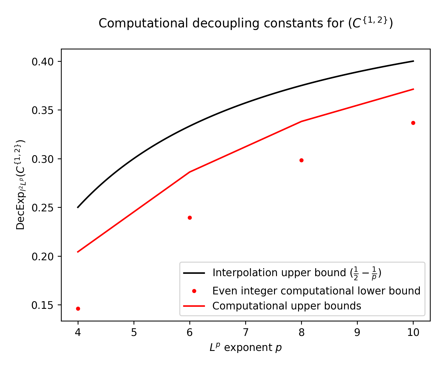
Refer to caption
Figure 3. Numerical estimation of α2​n​(ℰ3{1,2})\alpha_{2n}(\mathcal{E}_{3}^{\{1,2\}}). The optimization has been performed using gradient descent using Torch. At stopping time the l2l^{2} gradients of the optimization where ≤10−8\leq 10^{-8}. There is no guarantee, however, that the near-local-optimizers are in fact global optimizers of the problem at hand. The upper bounds on the figure (red line) are the upper bounds from 3.7 assuming the optimization problem resulted in a global optimizer.

Proposition 3.7 hints of a way of estimating the decoupling exponents of Cantor sets (or at least obtaining an upper bound) by computing the value of log⁡A2​n,1​([ℰq{d1,…,dk}]t)log⁡kt\frac{\log A_{2n,1}([{\mathcal{E}^{\{d_{1},\dots,d_{k}\}}_{q}}]_{t})}{\log k^{t}} for finite values of tt. Since [ℰq{d1,…,dk}]t[{\mathcal{E}^{\{d_{1},\dots,d_{k}\}}_{q}}]_{t} contains finitely many points, one may attempt to numerically find the extremizers to the decoupling inequality, in other words, to compute:

A2​n,1​([ℰq{d1,…,dk}]t)2​n\displaystyle A_{2n,1}([{\mathcal{E}^{\{d_{1},\dots,d_{k}\}}_{q}}]_{t})^{2n} =arg​maxf∈l2​([ℰq{d1,…,dk}]t)‖f‖l2=1∑a1,…​an∈[ℰq{d1,…,dk}]tb1,…​bn∈[ℰq{d1,…,dk}]ta1+⋯+an=b1+⋯+bnf(a1)…f(an)⋅f¯(b1)…f¯(bn)\displaystyle=\argmax_{\begin{subarray}{c}f\in l^{2}([{\mathcal{E}^{\{d_{1},\dots,d_{k}\}}_{q}}]_{t})\\ \|f\|_{l^{2}}=1\end{subarray}}\sum_{\begin{subarray}{c}a_{1},\dots a_{n}\in[{\mathcal{E}^{\{d_{1},\dots,d_{k}\}}_{q}}]_{t}\\ b_{1},\dots b_{n}\in[{\mathcal{E}^{\{d_{1},\dots,d_{k}\}}_{q}}]_{t}\\ a_{1}+\dots+a_{n}=b_{1}+\dots+b_{n}\end{subarray}}f(a_{1})\dots f(a_{n})\cdot\bar{f}(b_{1})\dots\bar{f}(b_{n})
(43) =arg​maxf∈l2​([ℰq{d1,…,dk}]t)‖f‖l2=1⁡‖f∗f​⋯∗f⏟n​ times‖l2​(ℤ)2\displaystyle=\argmax_{\begin{subarray}{c}f\in l^{2}([{\mathcal{E}^{\{d_{1},\dots,d_{k}\}}_{q}}]_{t})\\ \|f\|_{l^{2}}=1\end{subarray}}\|\underbrace{f\ast f\dots\ast f}_{n\text{ times}}\|_{l^{2}(\mathbb{Z})}^{2}

or, as an unconstrained optimization problem,

(44) A2​n,1​([ℰq{d1,…,dk}]t)=arg​maxsupp ​f⊆[ℰq{d1,…,dk}]t⁡‖f∗f​⋯∗f‖l2​(ℤ)1/n‖f‖l2​(ℤ)2A_{2n,1}([{\mathcal{E}^{\{d_{1},\dots,d_{k}\}}_{q}}]_{t})=\argmax_{\begin{subarray}{c}\text{supp }f\subseteq[{\mathcal{E}^{\{d_{1},\dots,d_{k}\}}_{q}}]_{t}\end{subarray}}\frac{\|{f\ast f\dots\ast f}\|_{l^{2}(\mathbb{Z})}^{1/n}}{\|f\|_{l^{2}(\mathbb{Z})}^{2}}

We performed the numerical optimization problem in (44) for the (0,2)mod3(0,2)\mod 3 Cantor set and n=1,2,3,4n=1,2,3,4 using gradient descent. The results can be seen in Figure 3. While there are no a priori guarantees that the near-local-optimizers obtained from gradient descent are in fact global optimizers of the problem at hand, this method was tested on the previous examples in Section 3.3, and converged to the known decoupling exponent.

3.4.1. A conjectured fixed point method

Studying equation (43), using Lagrange multipliers one may extract information about the solution, more precisely that, at extremizers (which must exist because l2​([ℰq{d1,…,dk}]t)l^{2}([{\mathcal{E}^{\{d_{1},\dots,d_{k}\}}_{q}}]_{t}) is a finite-dimensional space) the following equality holds:

f=λ⋅χ[ℰq{d1,…,dk}]t⋅∇‖f∗f​⋯∗f⏟n​ times‖l2​(ℤ)2f=\lambda\cdot\chi_{[{\mathcal{E}^{\{d_{1},\dots,d_{k}\}}_{q}}]_{t}}\cdot\nabla\|\underbrace{f\ast f\dots\ast f}_{n\text{ times}}\|_{l^{2}(\mathbb{Z})}^{2}

where ∇\nabla denotes the gradient with respect to ff in OPENl2​([ℰq{d1,…,dk}]t))l^{2}([{\mathcal{E}^{\{d_{1},\dots,d_{k}\}}_{q}}]_{t})). Let

Φ⁡(f):=λ⋅χ[ℰq{d1,…,dk}]t⋅∂∂f​‖f∗f​⋯∗f⏟n​ times‖l2​(ℤ)2.\Phi(f):=\lambda\cdot\chi_{[{\mathcal{E}^{\{d_{1},\dots,d_{k}\}}_{q}}]_{t}}\cdot\frac{\partial}{\partial f}\|\underbrace{f\ast f\dots\ast f}_{n\text{ times}}\|_{l^{2}(\mathbb{Z})}^{2}.

The functional Φ\Phi sends nonnegative functions to nonnegative functions, and by Cauchy-Schwarz we know there exists an extremizer with nonnegative components. This suggests the following numerical method to compute an extremizer:

TOL >0>0
f:χ[ℰq{d1,…,dk}]t→ℝ+f:\chi_{[{\mathcal{E}^{\{d_{1},\dots,d_{k}\}}_{q}}]_{t}}\to\mathbb{R}^{+}
n←0n\leftarrow 0
do
  fn+1←Φ⁡(fn)‖Φ⁡(fn)‖2f_{n+1}\leftarrow\frac{\Phi(f_{n})}{\|\Phi(f_{n})\|_{2}}
  n←n+1n\leftarrow n+1
while ‖fn−fn−1‖>\|f_{n}-f_{n-1}\|>TOL

Convergence of this algorithm to an unique maximum would follow if f↦Φ⁡(f)‖Φ⁡(f)‖f\mapsto\frac{\Phi(f)}{\|\Phi(f)\|} was contractive in some norm. Numerical experiments seem to indicate convergence of the algorithm in all situations that were tested at a much faster rate than the gradient descent methods.

3.4.2. Code

A commented version of the code can be found at https://github.com/jaumededios/Decoupling_Cantor.

References

  • [1] Kirsti D. Biggs, Efficient congruencing in ellipsephic sets: the general case, arXiv:1912.04351, 2019.
  • [2] by same author, Efficient congruencing in ellipsephic sets: the quadratic case, Acta Arith. 200 (2021), no. 4, 331–348.
  • [3] J. Bourgain, Bounded orthogonal systems and the Λ⁡(p)\Lambda(p)-set problem, Acta Math. 162 (1989), no. 3-4, 227–245.
  • [4] Jean Bourgain and Ciprian Demeter, The proof of the l2l^{2} decoupling conjecture, Ann. of Math. (2) 182 (2015), no. 1, 351–389.
  • [5] by same author, A study guide for the l2l^{2} decoupling theorem, Chin. Ann. Math. Ser. B 38 (2017), no. 1, 173–200.
  • [6] Jean Bourgain, Ciprian Demeter, and Larry Guth, Proof of the main conjecture in Vinogradov’s mean value theorem for degrees higher than three, Ann. of Math. (2) 184 (2016), no. 2, 633–682.
  • [7] Ciprian Demeter, A decoupling for Cantor-like sets, Proc. Amer. Math. Soc. 147 (2019), no. 3, 1037–1050.
  • [8] Javier Duoandikoetxea, Fourier analysis, Graduate Studies in Mathematics, vol. 29, American Mathematical Society, Providence, RI, 2001, Translated and revised from the 1995 Spanish original by David Cruz-Uribe.
  • [9] Semyon Dyatlov and Long Jin, Resonances for open quantum maps and a fractal uncertainty principle, Comm. Math. Phys. 354 (2017), no. 1, 269–316.
  • [10] Shaoming Guo, Zane Kun Li, and Po-Lam Yung, A bilinear proof of decoupling for the cubic moment curve, Trans. Amer. Math. Soc. 374 (2021), no. 8, 5405–5432.
  • [11] Shaoming Guo, Zane Kun Li, Po-Lam Yung, and Pavel Zorin-Kranich, A short proof of ℓ2\ell^{2} decoupling for the moment curve, American J. Math. 143 (2021), no. 6, 1983–1998.
  • [12] Larry Guth, 18.118 Topics in Analysis: Decoupling, Lecture 2, http://math.mit.edu/~lguth/Math118/DecLect2.pdf.
  • [13] Kathryn E. Hare and Ivo Klemes, On permutations of lacunary intervals, Trans. Amer. Math. Soc. 347 (1995), no. 10, 4105–4127.
  • [14] D. R. Heath-Brown, The cubic case of Vinogradov’s mean value theorem – a simplified approach to Wooley’s “efficient congruencing”, arXiv:1512.03272, 2015.
  • [15] Izabella Łaba and Hong Wang, Decoupling and near-optimal restriction estimates for Cantor sets, Int. Math. Res. Not. IMRN (2018), no. 9, 2944–2966.
  • [16] Zane Kun Li, An l2l^{2} decoupling interpretation of efficient congruencing: the parabola, Rev. Mat. Iberoam. 37 (2021), no. 5, 1761–1802.
  • [17] Lillian B. Pierce, The Vinogradov mean value theorem [after Wooley, and Bourgain, Demeter and Guth], Astérisque Exposés Bourbaki 407 (2019), 479–564.
  • [18] Terence Tao, 247B, Notes 2: Decoupling theory, What’s new blog, https://terrytao.wordpress.com/2020/04/13/247b-notes-2-decoupling-theory/.
  • [19] Terence Tao and Van Vu, Additive combinatorics, Cambridge Studies in Advanced Mathematics, vol. 105, Cambridge University Press, Cambridge, 2006.
  • [20] Trevor D. Wooley, Nested efficient congruencing and relatives of Vinogradov’s mean value theorem, Proceedings of the London Mathematical Society 118 (2019), no. 4, 942–1016.