Partial Network Identifiability: Theorem Proof and Evaluation

Fig. 4 illustrates a triconnected component $\mathcal{T}$ with $\sigma$ vantages ($\sigma\geq 2$), where some of these $\sigma$ vantages may form conjugate pairs. For vertex cut $\{v_{1},v_{2}\}$ (which is a Type-0-VC), there exists a simple path $\mathcal{P}_{r}$ connecting $v_{1}$ and $v_{2}$ in the neighboring biconnected component $\mathcal{B}_{\mathcal{T}}$ within the parent biconnected component of $\mathcal{T}$ as $\mathcal{B}_{\mathcal{T}}$ contains at least 3 nodes. We know that $\mathcal{B}_{\mathcal{T}}$ connects to $\mathcal{T}$ via only $\{v_{1},v_{2}\}$; therefore, $\mathcal{P}_{1},\ldots,\mathcal{P}_{\sigma}$ do not have common nodes with $\mathcal{B}_{\mathcal{T}}$ except that $\mu_{i}$ ($i=1,\ldots,\sigma$) may equal $v_{1}$ ($v_{2}$). Hence, for virtual link $v_{1}v_{2}$, if it is used for identifying real links in $\mathcal{T}$ according to Theorem III.2 or III.3, then it can be replaced by $\mathcal{P}_{r}$ which is a simple path and can be abstracted as a real link in $\mathcal{T}$.

For the case that $\{v_{1},v_{2}\}$ forms a Type-$k$-VC ($k\geq 1$) and no agents (excluding $v_{1}$ and $v_{2}$) in $\mathcal{B}_{\mathcal{T}}$ are used for identifying $\mathcal{T}$, we can ignore these agents in $\mathcal{B}_{\mathcal{T}}$. Accordingly, this Type-$k$-VC is converted to a Type-0-VC. Therefore, the above argument applies to this special case, suggesting the existence of replacement path $\mathcal{P}_{r}$. $\blacksquare$

1) If vantage $\mu_{i}$ is an agent, then $\mu_{i}$-to-agent path is itself $\mu_{i}$ (i.e., a path containing only one node). This is a trivial case that $\mu_{i}$-to-agent path is internally vertex disjoint with all other vantage-to-agent paths.

2) For triconnected component $\mathcal{T}$ in biconnected component $\mathcal{B}$, if vantage $\mu_{i}$ is not an agent and $\mu_{i}$ is in a Type-1-VC, then let $\mu^{\prime}_{i}$ be the other node in this Type-1-VC, $\mathcal{P}$ the $\mu_{i}$-to-agent path, and $\mathcal{P}^{\prime}$ the $\mu^{\prime}_{i}$-to-agent path. If $\mu_{i}$ and $\mu^{\prime}_{i}$ form a conjugate pair, then $\mathcal{P}$ and $\mathcal{P}^{\prime}$ may have a common terminating-point (i.e., the agent). In this case, in addition to the common terminating-point $m^{\prime}$, if $\mathcal{P}$ and $\mathcal{P}^{\prime}$ must have another common node $w$ (an internal vertex in $\mathcal{P}$ and $\mathcal{P}^{\prime}$), then it implies that $\mu_{i}$ and $\mu^{\prime}_{i}$ cannot connect to $m^{\prime}$ if $w$ is deleted. $w$ therefore is a cut-vertex in $\mathcal{B}$, contradicting the assumption that $\mathcal{B}$ is a biconnected component. If $\mu_{i}$ and $\mu^{\prime}_{i}$ do not form a conjugate pair, then $\mu^{\prime}_{i}$ is an agent. In this case, $\mu^{\prime}_{i}$-to-agent path is $\mu^{\prime}_{i}$, which is internally vertex disjoint with $\mathcal{P}$.

3) For triconnected component $\mathcal{T}$ in biconnected component $\mathcal{B}$, if vantage $\mu_{i}$ is not an agent and $\mu_{i}$ is in a Type-$k$-VC ($k\geq 2$), then we can always construct $\mu_{i}$-to-$m^{\prime}$ path $\mathcal{P}$ and $\mu^{\prime}_{i}$-to-$m^{\prime}$ path $\mathcal{P}^{\prime}$ ($\mu^{\prime}_{i}$ is another node in this Type-$k$-VC, suppose $\mu^{\prime}_{i}$ is not an agent) to make sure that $\mathcal{P}$ and $\mathcal{P}^{\prime}$ have the same terminating-point $m^{\prime}$. Then the same argument in 2) applies to this case.

4) In 2) and 3), we only consider constructing $\mathcal{P}$ and $\mathcal{P}^{\prime}$ in the same neighboring biconnected component $\mathcal{B}_{N}$ of $\mathcal{T}$. For the vantage-to-agent paths in other neighboring biconnected component of $\mathcal{T}$, these paths do not use any nodes in $\mathcal{B}_{N}$ (except for the possible case that the starting-point, i.e., the vantage, is in $\mathcal{B}_{N}$). Thus, these vantage-to-agent paths are still internally vertex disjoint with $\mathcal{P}$.

Therefore, for vantages in the same Type-$k$-VC, their vantage-to-agent paths at most have one common terminating-point (i.e., the agent). While for vantages in different Type-$k$-VCs, their vantage-to-agent paths at most have a common starting-point (i.e., the vantage). Consequently, For all vantages $\{\mu_{i}\}$ in $\mathcal{T}$, there exists an external $\mu_{i}$-to-agent path $\mathcal{P}$ which is internally vertex disjoint with all other $\mu_{j}$-to-agent paths ($j\neq i$). $\blacksquare$

It is easy to see that Categories 1–3 are mutually exclusive and cover all possibilities except for the case containing 0 or 1 vantage. If $\mathcal{T}$ only has 0 or 1 vantage, then $\mathcal{B}$ can only have 0 or 1 agent located in $\mathcal{T}$, as any other agent outside $\mathcal{T}$ will imply at least two vantages in $\mathcal{T}$ (nodes in the 2-vertex cut separating $\mathcal{T}$ from the agent must be vantages). Therefore, any triconnected component with the parent biconnected component containing 2 or more agents falls into one of Categories 1–3. $\blacksquare$

For real link $l_{i}$ in triconnected component $\mathcal{T}$, let $v_{1}$ and $v_{2}$ be the end-points of $l_{i}$, $v_{3}$ the third node in $\mathcal{T}$, $S_{1}$ ($S_{2}$) the set of immediately neighboring triconnected components connected to $\mathcal{T}$ via $\{v_{1},v_{3}\}$ ($\{v_{2},v_{3}\}$), and $S^{*}_{1}$ ($S^{*}_{2}$) the set of immediately neighboring biconnected components connected to $\mathcal{T}$ via $\{v_{1},v_{3}\}$ ($\{v_{2},v_{3}\}$) within the same parent biconnected component. Note all links in $S^{*}_{1}$ ($S^{*}_{2}$) except for $v_{1}v_{3}$ ($v_{2}v_{3}$) are real links. It suffices to show how the identifiability of $l_{i}$ is determined by Algorithm 1. Let $\mathcal{T}^{*}_{1}$ ($\mathcal{T}^{*}_{2}$) be a neighboring triconnected component of $\mathcal{T}$ with the following properties: (i) $v_{1}\in\mathcal{T}^{*}_{1}$ ($v_{2}\in\mathcal{T}^{*}_{2}$); (ii) $v_{2}\notin\mathcal{T}^{*}_{1}$ ($v_{1}\notin\mathcal{T}^{*}_{2}$); (iii) $\mathcal{T}^{*}_{1}$ ($\mathcal{T}^{*}_{2}$) contains at least two real links which are incident to $v_{1}$ ($v_{2}$); (iv) $\mathcal{T}^{*}_{1}$ ($\mathcal{T}^{*}_{2}$) contains 3 or more vantages.

We first consider the condition (called Condition A in the sequel) that: (a) $v_{1}v_{3}$ is virtual AND (b) $v_{1}$ is not an agent in the parent biconnected component of $\mathcal{T}$ AND (c) $\{v_{1},v_{2}\}$ is a Type-0-VC w.r.t. $\mathcal{T}$ if $\{v_{1},v_{2}\}$ is a 2-vertex cut AND (d) $|S_{1}|=1$ AND (e) $\mathcal{T}^{*}_{1}$ satisfying the properties (i)–(iv) does not exist. We show that if $\mathcal{T}$ does not satisfy any of the five conditions (a)–(e) in Condition A, then there exists a path replacement for $v_{1}v_{3}$ (denoted by $\mathcal{P}(v_{1},v_{r})$), one $v_{1}$-to-agent path, and one $v_{r}$-to-agent path, with all these three paths being internally vertex disjoint.

1. 1)

   If $v_{1}v_{3}$ is a real link, then it is obvious that there is no need to find a path replacement for $v_{1}v_{3}$. Moreover, according to the definition of Category 2.1, there exist two vantage-to-agent (i.e., $v_{1}$-to-agent and $v_{3}$-to-agent) disjoint paths;

2. 2)

   If $v_{1}$ is an agent in the parent biconnected component of $\mathcal{T}$, then $v_{1}$ itself is a degenerated $v_{1}$-to-agent path (containing a single node). In this case, if $S^{*}_{1}$ contains one agent (excluding $v_{1}$), say $m^{\prime}_{1}$ (as illustrated in Fig. 5), then there exist internally vertex disjoint paths $m^{\prime}_{1}e_{1}v_{1}$ and $m^{\prime}_{1}e_{2}v_{3}$ since each component in $S^{*}_{1}$ is 2-vertex-connected. Hence, $m^{\prime}_{1}e_{1}v_{1}$ can be used as the path replacement for $v_{1}v_{3}$. Note that $m^{\prime}_{1}e_{2}v_{3}$ might be merged with another path for identifying $v_{1}v_{2}$, which will be clear in later discussions. If $S^{*}_{1}$ does not contain any agents except for $v_{1}$, then there exists path replacement connecting $v_{1}$ and $v_{3}$ within $S^{*}_{1}$. Furthermore, for this replacement path, the end-point $v_{3}$ has a vantage-to-agent path in $S^{*}_{2}$ or $v_{3}$ itself is an agent according to the definition of Category 2.1.

   

3. 3)

   If $\{v_{1},v_{2}\}$ is a Type-$k$-VC ($k\geq 1$) w.r.t. $\mathcal{T}$ when $\{v_{1},v_{2}\}$ is a 2-vertex cut, then, as illustrated in Fig. 6, $v_{1}v_{2}$ is a Cross-link [3], which is identifiable using paths $\mathcal{P}_{1},\ldots,\mathcal{P}_{4}$ (see [3]).

4. 4)

   If $|S_{1}|>1$, then it implies $|S^{*}_{1}|>1$. Thus, the path replacement for $v_{1}v_{3}$ can be chosen from one component in $S^{*}_{1}$ and there exist $v_{1}$-to-agent ($v_{3}$-to-agent) path in another component of $S^{*}_{1}$.

   

5. 5)

   Suppose there exists $\mathcal{T}^{*}_{1}$ satisfying the properties in (i)–(iv). This is the most complicated condition in Condition A. Let $\mathcal{B}$ denote the parent biconnected component of $\mathcal{T}$. If we remove the neighboring biconnected component (except for nodes $v_{1}$ and $v_{2}$) connecting to $\mathcal{T}$ via $v_{1}v_{2}$, then, as illustrated in Fig.7, $v_{3}$ is a cut-vertex in the remaining graph $\mathcal{B}^{*}$. In $\mathcal{B}^{*}$, for the connected component containing $v_{1}$ and $v_{3}$, there exists a subgraph $\mathcal{B}_{1}$ which is 2-vertex-connected or a bond³³ 3 A bond is a graph with only two nodes and one link connecting these two nodes., as illustrated in Fig.7. Note that in Fig.7, all links in $\mathcal{B}_{1}$ and $\mathcal{B}_{2}$ are real links since they are 2-vertex-connected (or bonds), and $\mathcal{B}_{1}$ contains $\mathcal{B}_{2}$ when $v_{3}$ is the only cut-vertex in $\mathcal{B}^{*}$. Suppose (a)–(d) in Condition A are satisfied. If there exist real links $v_{1}v_{4}$ and $v_{1}v_{5}$ in $\mathcal{B}_{1}$, then $\mathcal{T}^{*}_{1}$ must be a subgraph in $\mathcal{B}_{1}$. Since $v_{2}$ and $v_{3}$ are vantages of $\mathcal{T}$, $v_{1}$ and $v_{4}$ must be the two vantages of $\mathcal{T}^{*}_{1}$. If $\mathcal{T}^{*}_{1}$ contains a third vantage, then it implies that there exists an agent $m^{\prime}_{1}$ (with $m^{\prime}_{1}\neq v_{1}$, $m^{\prime}_{1}\neq v_{4}$) in $\mathcal{B}_{1}$. Hence, as $\mathcal{B}_{1}$ is 2-vertex-connected, there exist internally vertex disjoint paths $v_{1}e_{1}m^{\prime}_{1}$ and $v_{1}v_{4}e_{2}v_{3}$. Therefore, $v_{1}v_{4}e_{2}v_{3}$ is chosen as the path replacement for $v_{1}v_{3}$. Moreover, there exist $v_{3}$-to-agent path (guaranteed by Condition B discussed as follows) in $S^{*}_{2}$ or $v_{3}$ itself is an agent in $\mathcal{B}$.

Let Condition B be (a) $v_{2}v_{3}$ is virtual AND (b) $v_{2}$ is not an agent in the parent biconnected component of $\mathcal{T}$ AND (c) $\{v_{1},v_{2}\}$ is a Type-0-VC w.r.t. $\mathcal{T}$ if $\{v_{1},v_{2}\}$ is a 2-vertex cut AND (d) $|S_{2}|=1$ AND (e) $\mathcal{T}^{*}_{2}$ satisfying the properties in (i)–(iv) does not exist. The above argument in 1)–5) also applies to the path replacement for $v_{2}v_{3}$. If neither Condition A nor Condition B is satisfied, then the two path replacements for $v_{1}v_{3}$ and $v_{2}v_{3}$ can be abstracted as two single links, thus forming a triangle containing link $v_{1}v_{2}$. Moreover, there exist vertex disjoint vertex-to-agent paths for the three vertices in this constructed triangle. Therefore, $v_{1}v_{2}$ is identifiable since the resided triangle with three vertex-to-agent paths (abstracting paths as single links) satisfies the condition in Theorem III.3.

Remark: When neither Condition A nor Condition B is satisfied, there are two other possible scenarios. (i) As shown in Fig. 5, if the replacement path for $v_{2}v_{3}$ is $v_{2}e_{3}v_{3}$, then $m^{\prime}_{1}e_{2}v_{3}+v_{3}e_{3}v_{2}$ can be abstracted as a single link in a triangle; (ii) In the case that $v_{1}$ and $v_{2}$ are both agents, if the replacement path for $v_{2}v_{3}$ is $m^{\prime}_{2}e_{5}v_{2}$ or $v_{3}$ itself is an agent, then a quadrangle (i.e., $(\{m^{\prime}_{1},v_{1},v_{2},m^{\prime}_{2}\},\{m^{\prime}_{1}e_{1}v_{1},v_{1}v_{2},v_{2}e_{5}m^{\prime}_{2},m^{\prime}_{1}v_{3}m^{\prime}_{2}\})$ or $(\{m^{\prime}_{1},v_{1},v_{2},v_{3}\},\{m^{\prime}_{1}e_{1}v_{1},v_{1}v_{2},v_{2}e_{3}v_{3},m^{\prime}_{1}e_{2}v_{3}\}$, where paths are abstracted as single links) is formed. Nevertheless, this quadrangle with its vertex-to-agent paths (abstracting paths as single links) also satisfies the condition in Theorem III.3.

If (a)–(e) in Condition A are satisfied, then it implies that $|S^{*}_{1}|=1$ and there is no agent (except for $v_{4}$) in $\mathcal{B}_{1}$ (see Fig. 7). Therefore, we can at most identify the sum metric of $v_{1}v_{2}$ and a path within $\mathcal{B}_{1}$, but not the individual link metric on $v_{1}v_{2}$. Same argument applies when (a)–(e) in Condition B are satisfied. Therefore, the identifiability of $l_{i}$ (with end-points $v_{1}$ and $v_{2}$) of Category 2.1 can be determined by Algorithm 1. $\blacksquare$

Let the two conjugate pairs be $\{\mu_{1},\mu_{2}\}$ and $\{\mu_{1},\mu_{3}\}$ and $S_{1}$ ($S_{2}$) the set of immediately neighboring triconnected components connecting to $\mathcal{T}$ via $\{\mu_{1},\mu_{2}\}$ ($\{\mu_{1},\mu_{3}\}$), as illustrated in Fig. 8. Since $\{\mu_{1},\mu_{2}\}$ and $\{\mu_{1},\mu_{3}\}$ are 2-vertex-cuts, we know that there exist internally vertex disjoint paths $\mathcal{P}_{1}$, $\mathcal{P}_{2}$, $\mathcal{P}_{3}$ and $\mathcal{P}_{4}$. If $\mu_{1}\mu_{2}$ (or $\mu_{1}\mu_{3}$) is a real link, then $\mu_{1}\mu_{2}$ (or $\mu_{1}\mu_{3}$) is known as a Cross-link [3] since $\mu_{2}\mu_{3}$ can be replaced by a path in neighboring biconnected components if $\mu_{2}\mu_{3}$ is virtual. Therefore, $\mu_{1}\mu_{2}$ (or $\mu_{1}\mu_{3}$) is identifiable. Now we focus on the identification of $\mu_{2}\mu_{3}$ in $\mathcal{T}$ (when $\mu_{2}\mu_{3}$ is a real link). The conditions to guarantee the identifiability of $\mu_{2}\mu_{3}$ is:
(link $\mu_{1}\mu_{2}$ is real OR $|S_{1}|\geq 2$ OR one component in $S_{1}$ is 3-vertex-connected) AND (link $\mu_{1}\mu_{3}$ is real OR $|S_{2}|\geq 2$ OR one component in $S_{2}$ is 3-vertex-connected).
Suppose the above condition is not satisfied. Then we can prove $\mu_{2}\mu_{3}$ is unidentifiable as follows.

We first consider the condition: link $\mu_{1}\mu_{3}$ is real OR $|S_{2}|\geq 2$ OR one component in $S_{2}$ is 3-vertex-connected. If not satisfied, then it implies that there is no real link $\mu_{1}\mu_{3}$ and the only immediately neighboring triconnected component is a triangle, i.e., $\mu_{1}$-$a$-$\mu_{3}$ in Fig. 9 ($\mu_{1}a$ and $\mu_{3}a$ can be virtual links as well).

1) If agent $m^{\prime}_{2}$ is in the location shown in Fig. 9(a), then all paths from $m^{\prime}_{1}$ to $m^{\prime}_{2}$ traversing $\mu_{2}\mu_{3}$ must use one simple path in $\mathcal{D}_{1}$. Therefore, the best case is that we can compute the sum metric of link ${\mu_{2}\mu_{3}}$ and another link which is incident to $\mu_{3}$ in $\mathcal{D}_{1}$, but cannot compute them separately.

2) If agent $m^{\prime}_{2}$ is in the location shown in Fig. 9(b), then $\mathcal{P}_{3}$ and $\mu_{2}\mu_{3}$ become a “double bridge” connecting $\mathcal{D}_{2}$ and $\mathcal{D}_{1}$. Abstracting $\mathcal{P}_{3}$ as a single link, [3] proves that none of the links in a double bridge is identifiable when constraining the measurement paths to simple paths. If we choose other paths as $\mathcal{P}_{3}$ in $\mathcal{D}_{3}$, then the same argument applies. Therefore, based on 1) and 2), $\mu_{2}\mu_{3}$ is unidentifiable.

Analogously, we can prove that $\mu_{2}\mu_{3}$ is unidentifiable when condition (link $\mu_{1}\mu_{2}$ is real OR $|S_{1}|\geq 2$ OR one component in $S_{1}$ is 3-vertex-connected) is not satisfied.

When the required conditions are satisfied, we can prove that $\mu_{2}\mu_{3}$ is identifiable as follows:

If $\mu_{1}\mu_{2}$ ($\mu_{1}\mu_{3}$) is a virtual link, then it can be replaced by a path in a neighboring component. For instance, if $|S_{1}|\geq 2$, then one replacement path can be found in one component of $S_{1}$. If one component in $S_{1}$ is 3-vertex-connected, then there exist 2 internally vertex disjoint paths (each with the order greater than 1) connecting $\mu_{1}$ and $\mu_{2}$. Thus, we can choose one of them as a replacement path. Note that the virtual links possibly involved in the replacement paths can be further replaced by the paths in their neighboring components within the same parent biconnected component. After these replacement operations, $\mu_{2}\mu_{3}$ in Fig. 8 is a Shortcut (defined in [3]), which is proved to be identifiable in [3].

Therefore, Algorithm 2 can determine all identifiable/unidentifiable links in a triangle triconnected component of Category 2.3. $\blacksquare$

For direct link $\mu_{1}\mu_{2}$ in $\mathcal{T}$, if there exist neighboring triconnected components connecting to $\mathcal{T}$ by 2-vertex cut $\{\mu_{1},\mu_{2}\}$ AND $\mu_{1}$ and $\mu_{2}$ are not the (only two) vantages in one of these neighboring components $\mathcal{T}_{N}$, then $\mu_{1}\mu_{2}$ is not a direct link connecting two vantages in $\mathcal{T}_{N}$. Therefore, if $\mathcal{T}_{N}$ is of Category 1 or 2, then Algorithm DAIL can determine the identifiability of $\mu_{1}\mu_{2}$; if $\mathcal{T}_{N}$ is of Category 3, then $\mu_{1}\mu_{2}$ is identifiable since it is not a direct link in $\mathcal{T}_{N}$. The above argument is complete, since the number of vantages in $\mathcal{T}_{N}$ cannot be less than 2 as the parent biconnected component of $\mathcal{T}$ (and $\mathcal{T}_{N}$) contains at least 2 agents⁴⁴ 4 In Algorithm 2, we only consider the biconnected components with 2 or more agents..

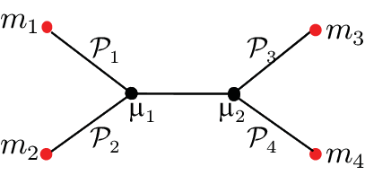
If the condition in line 1 of Algorithm B is not satisfied, then there is no neighboring triconnected component connecting to $\mathcal{T}$ by 2-vertex cut $\{\mu_{1},\mu_{2}\}$, or all these neighboring components contain only $\mu_{1}$ and $\mu_{2}$ as vantages, shown in Fig. 10. In this case, the identifiability of $\mu_{1}\mu_{2}$ can be determined with the assistance of neighboring biconnected components. Let $\mathcal{B}_{1}$ be the only biconnected component connecting to $\mathcal{T}$ via $\mu_{2}$, as shown in Fig. 10. Suppose $\mu_{2}$ is not a real monitor and $v_{1}$ is the only agent (except for $\mu_{2}$) in $\mathcal{B}_{1}$. Then we can at most identify the sum metric of $\mu_{1}\mu_{2}$ and a path connecting $\mu_{2}$ and $v_{1}$ in $\mathcal{B}_{1}$, but not the individual link metric on $\mu_{1}\mu_{2}$. Therefore, if $\mathcal{B}_{1}$ is the only biconnected component connecting to $\mathcal{T}$ by $\mu_{2}$ and $\mu_{2}$ is not a real monitor, then $\mathcal{B}_{1}$ must contain at least 2 agents (except for $\mu_{2}$) for identifying $\mu_{1}\mu_{2}$. The same argument applies to the biconnected components connecting to $\mathcal{T}$ via $\mu_{1}$. Suppose none of $\mu_{1}$ or $\mu_{2}$ is a real monitor. If there are more than one biconnected component connecting to $\mathcal{T}$ via $\mu_{1}$ (or $\mu_{2}$), e.g., $\mathcal{B}_{2}$ and $\mathcal{B}_{3}$ in Fig. 10, then the total number of agents (except for $\mu_{1}$ (or $\mu_{2}$)) must be no less than 2 for identifying $\mu_{1}\mu_{2}$. If these required conditions regarding neighboring biconnected components of $\mu_{1}$ and $\mu_{2}$ are satisfied, then this scenario can be abstracted as Fig. 11, which satisfies the condition (suppose $\mu_{1}$ and $\mu_{2}$ are not monitors) in Theorem III.3, and thus $\mu_{1}\mu_{2}$ is identifiable. Note that for node $\mu_{1}$, if $\mu_{1}$ is a real monitor, then there is no requirement for the neighboring biconnected components of $\mu_{1}$, since the subgraph containing $\mu_{1}\mu_{2}$, $\mathcal{P}_{3}$, $\mathcal{P}_{4}$ and their associated end-points also satisfies the condition in Theorem III.3. The same argument applies to the case when $\mu_{2}$ is a real monitor. Consequently, Algorithm B can determine the identifiability of $\mu_{1}\mu_{2}$ when the condition in line 1 is not satisfied, whereas the case satisfying the condition in line 1 can be determined in neighboring triconnected components (see line 2 of Algorithm B). $\blacksquare$

1) In [4], it has proved (see Lemma 2 in [4]) that 3-vertex-connected and single-link components in a graph decomposition are unique. Moreover, Lemma 2 in [4] also proved that if we merge (see Definition 2) all triangle components as much as possible, then a set of polygons are obtained and these polygons are unique. Since there are multiple ways to decompose a polygon, the generated triangle components may not be unique.

2) To prove the total number of triconnected components $\mathcal{N}_{\mathcal{T}}$ in $\mathcal{G}$ is fixed, it suffices to show that the total number of triangle components is fixed regardless of the mechanisms being used for graph decomposition, since all other types of triconnected components are unique as proved in 1). To this end, we have one claim: for a unique polygon $\mathcal{D}$ obtained in 1) with $\tau$ nodes ($\tau\geq 3$), the number of triangles after graph decomposition on $\mathcal{D}$ is always $\tau-2$, which is irrespective of decomposition strategies. We prove this claim by induction. (1) If $\tau=3$, then there is no need to further decompose $\mathcal{D}$, since $\mathcal{D}$ is already a triangle. Hence, in this case, the number of triangles is only one, i.e., $\tau-2$. (2) Suppose the claim is true for $\tau=k$ ($k$ is an integer, $k\geq 3$). (3) Consider the case that $\tau=k+1$. Fig. 12(a)–(b) display a polygon with $k+1$ nodes. For real link $w_{1}w_{2}$ on this polygon, after decomposition, it must belong to one triangle $\mathcal{T}$. Let the third node on $\mathcal{T}$ be $v$ (see Fig. 12(a)–(b)). Then there are two cases for $\mathcal{T}$: (i) $vw_{2}$ (or $vw_{1}$) is a real link in the original graph (Fig. 12(a)). In this case, excluding triangle $\mathcal{T}$, the remaining graph is polygon $\mathcal{D}_{1}$ with virtual link $vw_{1}$ (or $vw_{2}$). Then to get all triangles, $\mathcal{D}_{1}$ needs to be further decomposed. We know $|V(\mathcal{D}_{1})|=k$, and thus it corresponds to $k-2$ triangles according to the hypothesis in (2). Therefore, the total number of triangles is $(k+1)-2$; (ii) neither $vw_{1}$ nor $vw_{2}$ is a real link in the original graph $\mathcal{D}$. Then excluding triangle $\mathcal{T}$, the remaining graphs are $\mathcal{D}_{1}$ and $\mathcal{D}_{2}$ (Fig. 12(b)). To further decompose $\mathcal{D}_{1}$ and $\mathcal{D}_{2}$, we can first combine $\mathcal{D}_{1}$ and $\mathcal{D}_{2}$ as follows: Let $w_{1}=w_{2}$. The graph combination $\mathcal{D}^{\prime}$ is the union of $\mathcal{D}_{1}$ and $\mathcal{D}_{2}$, excluding virtual link $vw_{1}$ ($vw_{2}$) (see Fig. 12(c)). Then the decomposition of $\mathcal{D}_{1}$ and $\mathcal{D}_{2}$ is equivalent to the decomposition of $\mathcal{D}^{\prime}$, conditioned on that the vertex-cut $\{v,w_{1}\}$ (the same as $\{v,w_{2}\}$) must be used. We know the generated $\mathcal{D}^{\prime}$ is a polygon, which contains $k$ nodes, and thus it always corresponds to $k-2$ triangles (including the case that vertex-cut $\{v,w_{1}\}$ ($\{v,w_{2}\}$) must be used). Therefore, original graph $\mathcal{D}$ corresponds to $(k+1)-2$ triangles, completing the proof. $\blacksquare$

In Theorem III.2 and III.3, the prerequisite for network identifiability is that all involved links can be used for constructing measurement paths. In DAIL, we sequentially consider each triconnected component which possibly contains virtual links. These virtual links, however, do not exist in real networks. To tackle with this issue, Claim 1 states that a replacement path can be found for a virtual link whose end-points $\{v_{1},v_{2}\}$ form a Type-0-VC wrt $\mathcal{T}$. We will discuss the virtual links, not covered by Claim 1, in the following link identifications for the three (where there are four sub-categories for Category 2) triconnected component categories.

1) Category 1.

It suffices to only consider the case of a triconnected component $\mathcal{T}$ with 4 vantages. This is because, for a triconnected component $\mathcal{T}$ with more than 4 vantages, only four of them are useful for identifying $\mathcal{T}$. Since $|V(\mathcal{T})|\geq 4$, $\mathcal{T}$ must be 3-vertex-connected, i.e., not a triangle nor a bond. There are 3 possible scenarios after replacing all possible virtual links (according to Claim 1) in $\mathcal{T}$ by the corresponding real paths in neighboring components. (i) For the four vantages, each vantage-to-agent path is within a different biconnected component: As illustrated in Fig. 13(a), there exist 4 vertex disjoint vantage-to-agent paths $\mathcal{P}_{1},\ldots,\mathcal{P}_{4}$. Therefore, abstracting $\mathcal{P}_{1},\ldots,\mathcal{P}_{4}$ as single links, the graph in Fig. 13(a) satisfies the condition in Theorem III.3, and thus $\mathcal{T}$ is fully identifiable. (ii) For two vantages in $\{\mu_{1},\ldots,\mu_{4}\}$, say $\mu_{1}$ and $\mu_{2}$, their vantage-to-agent paths are within the same biconnected component, as shown in Fig. 13(b). In this case, there exists at least one agent ($m^{\prime}_{1}$) in the neighboring biconnected component $\mathcal{B}_{\mathcal{T}}$, and two internally vertex disjoint paths $\mathcal{P}_{1}$ and $\mathcal{P}_{2}$ in Fig. 13(b). Hence, abstracting $\mathcal{P}_{1},\ldots,\mathcal{P}_{4}$ in Fig. 13(b) as single links, the graph in Fig. 13(b) also satisfies the condition in Theorem III.3 even if $\mu_{1}\mu_{2}$ is a virtual link, and thus $\mathcal{T}$ is fully identifiable. (iii) For two pairs of vantages in $\{\mu_{1},\ldots,\mu_{4}\}$, the vantage-to-agent paths for each pair are within the same biconnected component, as shown in Fig. 13(c). Following the similar argument in (ii), the graph in Fig. 13(c) satisfies the condition in Theorem III.3 even if $\mu_{1}\mu_{2}$ and $\mu_{3}\mu_{4}$ are virtual links as $\mathcal{T}$ is 3-vertex-connected, and thus $\mathcal{T}$ is fully identifiable. On top of Fig. 13(c), there may exist other pairs of vantages, whose vantage-to-agent paths are within the same biconnected component. In this case, these vantage-to-agent paths can be ignored, since $\mathcal{P}_{1},\ldots,\mathcal{P}_{4}$ in Fig. 13(c) are already sufficient to identify $\mathcal{T}$.

2) Category 2.1.

Suppose $\mathcal{T}$ of Category 2.1 (Fig. 14) is 3-vertex-connected, and all possible virtual links in $\mathcal{T}$ are replaced by the corresponding real paths in neighboring components of $\mathcal{T}$. There are two possible scenarios. (i) For the three vantages, each vantage-to-agent path is within a different biconnected component: As illustrated in Fig. 14(a), there exist 3 vertex disjoint vantage-to-agent paths $\mathcal{P}_{1},\ldots,\mathcal{P}_{3}$. Therefore, abstracting $\mathcal{P}_{1},\ldots,\mathcal{P}_{3}$ as single links, the graph in Fig. 14(a) satisfies the condition in Theorem III.3, and thus $\mathcal{T}$ is fully identifiable. (ii) For two vantages in $\{\mu_{1},\ldots,\mu_{3}\}$, say $\mu_{2}$ and $\mu_{3}$, their vantage-to-agent paths are within the same biconnected component $\mathcal{B}_{\mathcal{T}}$, as shown in Fig. 14(b). In this case, there exist path $\mathcal{P}_{4}$ connecting $v_{1}$ and $v_{2}$, and $v_{1}$ ($v_{2}$) has at least 3 neighbors in $\mathcal{B}_{\mathcal{T}}$. Moreover, $\mu_{2}$ and $\mu_{3}$ must have at least two neighbors in $\mathcal{T}$ (we have assumed all other virtual links in $\mathcal{T}$ have been replaced by neighboring components), since $\mathcal{T}$ is 3-vertex-connected. Therefore, $\mu_{2}$ and $\mu_{3}$ are not nodes with only two neighbors, and thus they do not have to be monitors for complete network identification of Fig. 14(b) (see the explanation of MMP in [1]). Abstracting $\mathcal{P}_{1},\mathcal{P}_{21},\mathcal{P}_{22},\mathcal{P}_{31},\mathcal{P}_{32},\mathcal{P}_{4}$ in Fig. 14(b) as single links, the graph in Fig. 14(b) satisfies the condition in Theorem III.3 even if $\mu_{2}\mu_{3}$ is a virtual link, and thus 3-vertex-connected component $\mathcal{T}$ is fully identifiable. Meanwhile, same argument applies if $\{\mu_{1},\mu_{2}\}$ and/or $\{\mu_{1},\mu_{3}\}$ are type-$k$-VCs ($k\geq 2$).

References

- [1] L. Ma, T. He, K. K. Leung, A. Swami, and D. Towsley, “Monitor placement for maximal identifiability in network tomography,” in IEEE INFOCOM, 2014.
- [2] R. Diestel, Graph theory. Springer-Verlag Heidelberg, New York, 2005.
- [3] L. Ma, T. He, K. K. Leung, A. Swami, and D. Towsley, “Identifiability of link metrics based on end-to-end path measurements,” in ACM IMC, 2013.
- [4] J. E. Hopcroft and R. E. Tarjan, “Dividing a graph into triconnected components,” SIAM Journal on Computing, vol. 2, pp. 135–158, 1973.