Temperature dependent maximization of work and efficiency in a degeneracy assisted quantum Stirling heat engine

Sarbani Chatterjee Email: mp18015@iisermohali.ac.in Affiliation: Department of Physical Sciences, Indian Institute of Science Education and Research (IISER) Mohali, Sector 81 SAS Nagar, Manauli P.O. 140306 Punjab, India. Arghadip Koner Email: akoner@ucsd.edu Affiliation: Department of Chemistry and Biochemistry, University of California, San Diego, 9500 Gilman Dr, La Jolla, CA 92093, United States. Sohini Chatterjee Email: schatterjee@jncasr.ac.in Affiliation: Chemistry and Physics of Materials Unit, Jawaharlal Nehru Centre for Advanced Scientific Research (JNCASR), Jakkur P.O. Bangalore, 560064, India. Chandan Kumar Email: ph12129@iisermohali.ac.in Affiliation: Department of Physical Sciences, Indian Institute of Science Education and Research (IISER) Mohali, Sector 81 SAS Nagar, Manauli P.O. 140306 Punjab, India.

Abstract

We propose a quantum Stirling heat engine with an ensemble of harmonic oscillators as the working medium. We show that the efficiency of the harmonic oscillator quantum Stirling heat engine (HO-QSHE) at a given frequency can be maximized at a specific ratio of the temperatures of the thermal reservoirs. In the low temperature or equivalently high frequency limit of the harmonic oscillators, the efficiency of the HO-QSHE approaches the Carnot efficiency. Further, we analyse quantum Stirling heat engine with an ensemble of particle in box quantum systems as the working medium. Here both work and efficiency can be maximized at a specific ratio of temperatures of the thermal reservoirs. These studies will enable us to operate the quantum Stirling heat engines at its optimal performance. The theoretical study of the HO-QSHE would provide impetus for its experimental realisation, as most real systems can be approximated as harmonic oscillators for small displacements near equilibrium.

I Introduction

Thermodynamics started as an exact science at the length scales of macroscopic objects. The laws of classical thermodynamics were derived empirically and thus were more robust than any other theory of that time. One of the many practical aspects of this theory was to find the fundamental upper bound in the efficiency of heat engines Carnot 2005; Maxwell 1860; Boltzmann 1872, which are devices that utilise the spontaneous heat flow from a hot to a cold bath, and in the process, convert this heat into mechanical work. Today, the experimental advances in quantum physics have pushed the use of macroscopic thermodynamics and its partner, classical statistical mechanics, to even smaller length scales Klaers et al. 2017; Peterson et al. 2019. These advancements have led to a successful generalisation of the classical thermodynamic processes to their corresponding quantum versions Vinjanampathy and Anders 2016; Binder et al. 2019; Bhattacharjee and Dutta 2020. Quantum heat engines are ‘microscopic’ versions of the macroscopic thermodynamic cycles that capitalise on the ‘quantumness’ of the working system to generate positive work Binder et al. 2019.

The first proposed quantum heat engine was a three-level maser which operated with Carnot efficiency in the limiting case Scovil and Schulz-DuBois 1959. Using the generalisation from classical to quantum theory, the theoretical construction of quantum mechanical versions of various classical engines such as Otto, Carnot, Stirling, Brayton, and Diesel have been achieved Quan et al. 2007; Günter 2015; Quan 2009. A lot of work is in progress which looks forward to designing and deriving the optimal performances of quantum mechanical heat engines from microscopic mechanical laws Chen et al. 2020; Tajima and Hayashi 2017; Wang et al. 2009; Stefanatos 2014; Thomas et al. 2019; Wu et al. 2006; Dong et al. 2013. Quantum heat engines using non-markovian Zhang et al. 2014a, quantum coherent Scully et al. 2003; Quan et al. 2006, quantum squeezed Huang et al. 2012; Roßnagel et al. 2014; Klaers et al. 2017; Niedenzu et al. 2018; Wang et al. 2019, and entangled Dillenschneider and Lutz 2009 baths with efficiencies beyond the classical Carnot limit but with no violations to the second law of thermodynamics have also been proposed. While the extracted work and efficiency depend on the working media in a quantum heat engine, these properties are indifferent to the working media used in a classical heat engine. Different quantum mechanical working media, for instance, multi-level quantum systems Scovil and Schulz-DuBois 1959; Geva and Kosloff 1992; Harbola et al. 2012; Rahav et al. 2012; Hamedani Raja et al. 2020, particle in a box Su et al. 2018; Thomas et al. 2019, and harmonic oscillators Lin and Chen 2003a; Lin and Chen 2003b; Insinga et al. 2016; Kosloff and Rezek 2017, have already been employed in designing quantum heat engines.

In this article, we strive to construct a quantum heat engine whose working principle is exclusively based on the quantum features of formation of quantized energy levels and quantum degeneracies Gelbwaser-Klimovsky et al. 2018; Su et al. 2018; Thomas et al. 2019, owing to the finite boundary conditions Sakurai and Napolitano 2017. In this endeavour, we first propose a quantum Stirling heat engine based on an ensemble of quantum harmonic oscillators, where the degeneracy is generated by inserting a barrier in the middle of the harmonic oscillator. These degeneracies induce a lack of information, which can be converted to useful work using two reservoirs at different temperatures. We provide a rigorous study of work and efficiency in harmonic oscillator quantum Stirling heat engine (HO-QSHE), where the results show that the efficiency can be maximized at a specific ratio of hot and cold reservoir temperatures, and that this maximum depends on the frequency of the harmonic oscillator; however, there is no such maximum for the extracted work. We also study the quantum Stirling heat engine based on an ensemble of particle-in-a-box quantum systems. We discuss work and efficiency for both symmetric and asymmetric insertion of a single barrier and also the insertion of multiple barriers in particle in a box quantum Stirling heat engine (PIB-QSHE). The results reveal that both work and efficiency can be maximized at a certain specific ratio of hot and cold temperatures, which depends on the length of the box.

The motivation behind choosing a quantum harmonic oscillator as the working medium of the quantum heat engine is the fact that it is one of the most ubiquitous quantum systems, which models atoms in a lattice to quantum fields. Since almost any generic potential can be approximated as a harmonic oscillator for small displacements near equilibrium tay, our proposed degeneracy assisted HO-QSHE may be realised practically. Possible candidates include Bose-Einstein condensate, Josephson junction, and vibrational modes of solid Scharf et al. 2020; Barontini and Paternostro 2019; Paraoanu et al. 2001; Weedbrook et al. 2012. Similarly, quantum dots, wires, and wells are promising candidates for the realisation of the degeneracy assisted PIB-QSHE Sattler 2010.

We arrange the paper as follows. Sec. II describes the quantum Stirling heat engine based on harmonic oscillators. The work and efficiency for it are analyzed in Sec. III.1, while the results for a quantum Stirling engine based on an ensemble of particle in a box quantum systems is discussed in Sec. III.2. In Sec. IV, we discuss our results and future aspects of this work. Appendix A recapitulates the particle in a box Stirling heat engine.

II Harmonic oscillator based quantum Stirling heat engine

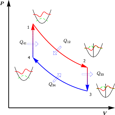
In this section, we propose a quantum Stirling heat engine with the working medium as a harmonic oscillator. Analogous to the classical counterpart, a quantum Stirling cycle is a four-stroke closed cycle regenerative heat engine. The schematic diagram of a classical Stirling heat cycle has been shown in Fig. 1. The corresponding processes for the quantum Stirling heat engine are also superposed on the same diagram.

Refer to caption — Figure 1: Schematic of the classical Stirling heat engine on a $PV$ diagram. The process $[(1)\rightarrow(2)]$ represents isothermal expansion of the system. The process $[(2)\rightarrow(3)]$ shows isochoric cooling of the engine when it is brought in contact with a reservoir at a lower temperature $T_{c}$ . The process $[(3)\rightarrow(4)]$ represents isothermal compression and $[(4)\rightarrow(1)]$ is the isochoric heating when the engine is connected back to the heat reservoir at temperature $T_{h}$ . The corresponding degeneracy assisted harmonic oscillator quantum Stirling heat engine is also depicted on the same diagram. Here, a barrier is inserted at the centre of the harmonic oscillator during the process $[(1)\rightarrow(2)]$ . Consequently, the even numbered energy levels are raised to the odd numbered energy levels and the final energy spectrum is doubly degenerate. The working medium during this process is constantly in equilibrium with the heat reservoir at temperature $T_{h}$ . During the process $[(2)\rightarrow(3)]$ the system is connected to the reservoir at a lower temperature $T_{c}$ and as a result heat is released from the system. In the process $[(3)\rightarrow(4)]$ , the barrier is removed quasi-statically from the harmonic oscillator while the Stirling heat engine is in equilibrium with a cold reservoir at temperature $T_{c}$ . In the final process of the cycle $[(4)\rightarrow(1)]$ , the system is brought in contact with the heat reservoir at temperature $T_{h}$ and heat is absorbed by the system.

The four steps involved in a HO-QSHE are as follows.

First step : In the first step of the quantum Stirling heat engine, a barrier is inserted at the centre of the harmonic oscillator in a quasi-static manner, thus allowing the system to be in constant equilibrium with the heat bath at temperature $T_{h}$ through heat exchange between the two. In contrast, the first step in a classical heat engine is that of isothermal expansion, where a system coupled to a heat bath at temperature $T_{h}$ expands isothermally (mechanical work is done by the system). It is worth mentioning that when we talk about the temperature of the system, we refer to the temperature of the ensemble of the working medium. For a one dimensional quantum harmonic oscillator of frequency $\omega$ as the working medium, the $n^{th}$ energy level is given as

E_{n}=\bigg(n+\frac{1}{2}\bigg)\hbar\omega\quad\text{with}\,n=0,1,2,\dots,

(1)

where $\hbar$ is the reduced Planck constant. This is the energy level spectra corresponding to the initial state for the first process of the HO-QSHE cycle (stage $1$ in Fig. 1). The partition function of the initial state $Z_{(1)}$ is given as

Z_{(1)}=\sum_{n=0}^{\infty}e^{-\frac{E_{n}}{k_{B}T_{h}}}=e^{\frac{-\hbar\omega}{2k_{B}T_{h}}}\sum_{n=0}^{\infty}e^{\frac{-n\hbar\omega}{k_{B}T_{h}}},

(2)

where $k_{B}$ is the Boltzmann constant. The partition function is a geometric sum which can be readily evaluated as

Z_{(1)}=\frac{e^{\frac{-\hbar\omega}{2k_{B}T_{h}}}}{1-e^{\frac{-\hbar\omega}{k_{B}T_{h}}}}=\frac{1}{2\sinh\bigg({\frac{\hbar\omega}{2k_{B}T_{h}}}\bigg)}.

(3)

The isothermal process involves the quasi-static insertion of a barrier in the centre of the harmonic oscillator. For this work, we assume that the centre of the potential is the origin of the coordinate system. This barrier is an infinite potential delta function ( $p\hskip 2.0pt\delta(0)$ , $p\to\infty$ ), which introduces an additional constraint of the probability amplitude of the wave function going to zero at the centre Griffiths 2005; Sørdal and Bergli 2019. A barrier inserted in this way does not alter the volume or the classical energy of the system but affects the quantum mechanical energy wave functions. The barrier ‘splits’ the wave functions into two exactly identical parts by introducing a node at their midpoints. Since the wave functions cannot vanish, the wave functions with even quantum numbers are ‘raised’ in energy to the next odd numbered energy state with the introduction of the barrier at the origin. The energy states with odd quantum numbers, are now two-fold degenerate (stage $2$ in Fig. 1). The new energy levels of this system are given as

E_{n}=\bigg(n+\frac{1}{2}\bigg)\hbar\omega\quad\text{with}\,n=1,3,5,\dots,

(4)

which could be alternatively written as

E_{n}=\bigg(2n+\frac{3}{2}\bigg)\hbar\omega\quad\text{with}\,n=0,1,2,\dots.

(5)

Various thermodynamics variables considered in this article are normalized to the number of particles in the ensemble, and therefore, will be intensive. Therefore, the partition function can be written as

Z_{(2)}=2e^{\frac{-3\hbar\omega}{2k_{B}T_{h}}}\sum_{n=0}^{\infty}e^{-\frac{2n\hbar\omega}{k_{B}T_{h}}}=\frac{2{e^{\frac{-3\hbar\omega}{2k_{B}T_{h}}}}}{\bigg(1-{e^{\frac{-2\hbar\omega}{k_{B}T_{h}}}}\bigg)}.

(6)

The internal energy at stage (1) of the Stirling cycle can be written in terms of the partition functions as $U_{(1)}=-\partial\ln Z_{(1)}/\partial\beta_{h}$ , where $\beta_{h}$ is $1/k_{B}T_{h}$ . Therefore, the change in the internal energy from stage $(1)$ to stage $(2)$ can be expressed as

\Delta U_{12}=U_{(2)}-U_{(1)}=-\frac{\partial}{\partial\beta_{h}}[\ln Z_{(2)}-\ln Z_{(1)}].

(7)

Further, the thermodynamic entropy at stage (1) can be expressed in terms of the partition functions as

S_{(1)}=k_{B}\left(1-\beta_{h}\frac{\partial}{\partial\beta_{h}}\right)\ln Z_{(1)}.

(8)

Therefore, the heat absorbed in the process of taking the system from state $(1)$ to state $(2)$ is given as $Q_{12}=T_{h}(S_{(2)}-S_{(1)})$ , which can be expressed as following using Eqs. (8) and (7):

	$\displaystyle Q_{12}$	$\displaystyle=\left(\frac{1}{\beta_{h}}-\frac{\partial}{\partial\beta_{h}}\right)[\ln Z_{(2)}-\ln Z_{(1)}],$		(9)
		$\displaystyle=U_{(2)}-U_{(1)}+k_{B}T_{h}\ln Z_{(2)}-k_{B}T_{h}\ln Z_{(1)}.$		(9)

We note that the change in internal energy $(U_{(2)}-U_{(1)})$ is not zero since the energy level spectra of the harmonic oscillator changes when the barrier is inserted. This is in contrast with the classical Stirling heat engine, where the internal energy remains constant during an isothermal process. This is because the energy level spectra of the working medium is the same throughout the cycle.

The work done in the process is given by first law of thermodynamics as

W_{12}=Q_{12}-\Delta U_{12}=k_{B}T_{h}\ln Z_{(2)}-k_{B}T_{h}\ln Z_{(1)}.

(10)

The work in this step is done by the system and hence is expected to be negative.

Second step : In this step, we connect the system to a thermal bath at temperature $T_{c}<T_{h}$ after disconnecting it from the thermal bath at temperature $T_{h}$ . Consequently, the temperature of the system falls down from $T_{h}$ to $T_{c}$ . This process for a classical Stirling heat engine is termed isochoric cooling, where the volume remains constant, and thus no mechanical work is done. Therefore, this process causes the system to lose heat.

The partition function of the initial state for this step is $Z_{(2)}$ . The partition function of the final state is exactly similar to $Z_{(2)}$ , since the energy spectra of the system remains the same, with the exception that here the temperature is $T_{c}$ instead of $T_{h}$ . The partition function is given as

Z_{(3)}=2e^{\frac{-3\hbar\omega}{2k_{B}T_{c}}}\sum_{n=0}^{\infty}e^{-\frac{2n\hbar\omega}{k_{B}T_{c}}}=\frac{2{e^{\frac{-3\hbar\omega}{2k_{B}T_{c}}}}}{\bigg(1-{e^{\frac{-2\hbar\omega}{k_{B}T_{c}}}}\bigg)}.

(11)

The amount of heat lost in this step can be calculated in terms of the partition function. Since no mechanical work is done ( $W_{23}=0$ ), the heat lost is equal to the change in internal energy:

Q_{23}=U_{(3)}-U_{(2)}=-\frac{\partial\ln Z_{(3)}}{\partial\beta_{c}}+\frac{\partial\ln Z_{(2)}}{\partial\beta_{h}}.

(12)

Third step : In the next step, the barrier is removed quasi-statically such that the system is in thermal equilibrium with the cold bath at temperature $T_{c}$ at all times. At the end of the process, the energy spectra become identical to that of the initial state $(1)$ . Again the volume remains constant for the quantum Stirling heat engine. In contrast, the corresponding step in a classical heat engine is that of isothermal compression, where a system coupled to a cold bath at temperature $T_{c}$ undergoes a compression. The partition function of the final state is same as that of $Z_{(1)}$ , but with temperature $T_{c}$ instead of $T_{h}$ :

Z_{(4)}=e^{\frac{-\hbar\omega}{2k_{B}T_{c}}}\sum_{n=0}^{\infty}e^{\frac{-n\hbar\omega}{k_{B}T_{c}}}=\frac{e^{\frac{-\hbar\omega}{2k_{B}T_{c}}}}{\bigg(1-{e^{\frac{-\hbar\omega}{k_{B}T_{c}}}}\bigg)}.

(13)

The heat provided to the system at the end of the process is obtained in terms of the partition functions as

Q_{34}=U_{(4)}-U_{(3)}+k_{B}T_{c}\ln Z_{(4)}-k_{B}T_{c}\ln Z_{(3)}.

(14)

The isothermal work done is obtained from the first law of thermodynamics as

W_{34}=Q_{34}-\Delta U_{34}=k_{B}T_{c}\ln Z_{(4)}-k_{B}T_{c}\ln Z_{(3)},

(15)

where $\Delta U_{34}=U_{(4)}-U_{(3)}$ is the change in internal energy in the process.

Fourth step : In the final step, the system is detached from the cold bath at temperature $T_{c}$ and connected to the hot bath at temperature $T_{h}$ . This raises the temperature of the system from $T_{c}$ to $T_{h}$ . The corresponding process for a classical Stirling heat engine is called isochoric heating, where the volume does not change, and therefore no mechanical work is done. Thus, the system loses heat during this process. Thus at the end of the process, the system returns to the initial state $(1)$ (the ensemble of harmonic oscillators at a temperature $T_{h}$ ). Since no work is done in this step, the heat absorbed by the system is equal to the change in internal energy:

Q_{41}=-\frac{\partial\ln Z_{(1)}}{\partial\beta_{h}}+\frac{\partial\ln Z_{(4)}}{\partial\beta_{c}}.

(16)

The four thermodynamic processes described above form one complete cycle of the quantum Stirling heat engine. The total work done by the system in one complete cycle of the HO-QSHE is given as

	$\displaystyle W_{\textrm{net}}$	$\displaystyle=$	$\displaystyle W_{12}+W_{34},$		(17)
		$\displaystyle=$	$\displaystyle k_{B}T_{h}\ln\frac{Z_{(2)}}{Z_{(1)}}+k_{B}T_{c}\ln\frac{Z_{(4)}}{Z_{(3)}}.$		(17)

Further, since the system absorbs heat only during the first isothermal step $[(1)\rightarrow(2)]$ and the final isochoric step $[(4)\rightarrow(1)]$ , the total heat absorbed during one complete cycle of the HO-QSHE can be written as

Q_{\textrm{in}}=Q_{12}+Q_{41}.

(18)

The efficiency $\eta$ for the cycle is given in terms of the work done and the heat intake as

\eta=\frac{W_{\textrm{net}}}{Q_{\textrm{in}}}=1+\frac{Q_{23}+Q_{34}}{Q_{12}+Q_{41}}.

(19)

The expression for the efficiency can be obtained from the partition functions and their derivatives.

III Analysis of work and efficiency

In this section, we first analyse the work and efficiency for HO-QSHE and then move on to PIB-QSHE.

III.1 Work and efficiency of the harmonic oscillator quantum Stirling heat engine

We first explore the work and efficiency of the HO-QSHE with respect to the frequency $\omega$ of the harmonic oscillator for different values of $T_{h}/T_{c}$ . For convenience, we introduce dimensionless units for the work extracted and the frequency by re-scaling them as $W/k_{B}T_{c}$ and as $\omega\hbar/k_{B}T_{c}$ respectively.

We define the harmonic oscillator of frequency $\omega$ to be in the low temperature limit, when the following condition is satisfied:

\hbar\omega>>k_{B}T_{h}\quad\text{with}\,\,T_{h}>T_{c}.

(20)

This condition is satisfied for large values of $\omega$ as well as very small values of $T_{h}$ .

As shown in Fig. 2(a), the work increases monotonically from zero as a function of the frequency of the harmonic oscillator and asymptotically approaches the high frequency limit, which can be derived using Eq. (17) to be $(T_{h}/T_{c}-1)\ln 2$ . This result can be numerically verified from the plot. Furthermore, as we increase the value of $T_{h}/T_{c}$ , the amount of extracted work increases.

Similarly, the efficiency also starts to rise from zero as the frequency increases and becomes asymptotic in the high frequency limit as shown in Fig. 2(b). We can derive this asymptotic efficiency value using Eq. (19) as $(1-T_{c}/T_{h})$ which can also be verified from the figure. Interestingly, this is the efficiency of a classical Carnot cycle. Thus, in the high frequency or low temperature limit, the efficiency of a HO-QSHE approaches the Carnot efficiency.

We note that efficiency curves for different values of $T_{h}/T_{c}$ cross over each other as the frequency is varied.

To analyse the explicit temperature dependence, we plot work and efficiency as a function of $T_{h}/T_{c}$ for different frequencies of the harmonic oscillator in Fig. 3. Here, the frequencies of the harmonic oscillator have been set to be integral multiples of $\omega_{0}\;(\omega=m\omega_{0})$ , where $\omega_{0}=k_{B}T_{c}/\hbar$ . The results show that the extracted work starts to increase from zero with increase in the value of $T_{h}/T_{c}$ and becomes asymptotic in the high $T_{h}/T_{c}$ limit. The asymptotic value of the net work extracted can be computed using Eq. (17) as

\lim\limits_{T_{h}/T_{c}\to\infty}W_{\textrm{net}}=k_{B}T_{c}\left(\ln\left[\frac{1+e^{m}}{2}\right]-\frac{m}{2}\right).

(21)

Therefore, the scaled work is given as $\ln[(1+e^{m})/2]-m/2$ , which can be numerically verified from the figure. On the other hand, the efficiency as a function of $T_{h}/T_{c}$ attains a maximum after a steep ascent and then gradually levels off to zero in the asymptotic limit. In contrast, the efficiency of a classical heat engine increases monotonically as a function of $T_{h}/T_{c}$ . We further notice from Fig. 3(b) that the efficiency approaches Carnot limit for small $T_{h}/T_{c}$ . This fact can be verified from Fig. 4, where we have plotted efficiency normalized by Carnot limit as a function of $T_{h}/T_{c}$ .

Furthermore, the monotonic decrease of the efficiency in Fig. 3(b) after the maxima and consequently the asymptotic decay to zero in the high $T_{h}/T_{c}$ limit can be attributed to the fact that as the ratio $T_{h}/T_{c}$ increases, more heat needs to be provided to the system to raise its temperature from $T_{c}$ to $T_{h}$ in the final step [ $(4)\rightarrow(1)$ ] of the Stirling cycle. This increases the value of total heat input $Q_{\textrm{in}}$ to the system. As can be seen from Fig. 5, the heat taken in during the isothermal process $Q_{12}$ also contributes to $Q_{\textrm{in}}$ , but its effect is small since there is no temperature change during this process.

Thus, because of the $Q_{41}$ term, $Q_{\textrm{in}}$ dominates over $W_{\textrm{{net}}}$ , consequently diminishing the efficiency of the cycle as per Eq. (19), and thus the efficiency approaches zero in the high $T_{h}/T_{c}$ limit.

It should be noted that the curves plotted as a function of $T_{h}/T_{c}$ start from $T_{h}/T_{c}=1$ , i.e., when both the reservoirs are at the same temperature, and hence no work is extracted. We have numerically computed the values of $T_{h}/T_{c}$ corresponding to the maximum efficiency for different harmonic oscillator frequencies and compared it with the Carnot efficiency at the corresponding values of $T_{h}/T_{c}$ in Table 1. The results show that although increasing the frequency initially leads to increase in the efficiency of the HO-QSHE, the rate of increase slows down and eventually saturates. Further, the efficiency for the HO-QSHE is bounded from above by the Carnot efficiency. The maximum efficiency asymptotically approaches unity as the frequency of the harmonic oscillator $\omega\rightarrow\infty$ . Furthermore, the unit efficiency is achieved for $T_{h}/T_{c}\rightarrow\infty$ as is for a Carnot engine. This behavior is reinforced by Fig. 3.

Table 1: Comparison of the numerical results for maximum efficiency of the HO-QSHE (

\eta_{\text{max}}

) and Carnot efficiency (

\eta_{\text{C}}

)

Frequency $\omega$	$T_{h}/T_{c}$	$\eta_{\text{max}}$	$\eta_{\text{C}}$
$5\,\omega_{0}$	2.66	0.47	0.62
$10\,\omega_{0}$	4.15	0.68	0.76
$15\,\omega_{0}$	5.58	0.77	0.82
$50\,\omega_{0}$	14.57	0.92	0.93
$150\,\omega_{0}$	36.93	0.97	0.97
$350\,\omega_{0}$	77.14	0.98	0.99

The cross over of the efficiency curves in Fig. 2(b) is a consequence of the existence of maxima in Fig. 3(b). We try to explain our point by comparing the value of efficiency at two different frequencies for different values of $T_{h}/T_{c}$ . For instance, the efficiency curve for $\omega=5\,\omega_{0}$ , which has a maximum at $T_{h}/T_{c}=2.66$ , takes the value $\eta=0.43$ , $0.46$ , and $0.41$ at $T_{h}/T_{c}=2$ , $3$ , and $4$ , respectively. Hence, at $\omega=5\,\omega_{0}$ , the efficiency is maximum for $T_{h}/T_{c}=3$ and minimum for $T_{h}/T_{c}=4$ , which can be confirmed from Fig. 2(b). Similarly, the efficiency curve for $\omega=10\,\omega_{0}$ takes the value $\eta=0.49$ , $0.64$ , and $0.68$ at $T_{h}/T_{c}=2$ , $3$ , and $4$ , respectively. Hence, the efficiency is maximum for $T_{h}/T_{c}=4$ and minimum for $T_{h}/T_{c}=2$ at $\omega=10\,\omega_{0}$ . These changes in the ordering of the numerical values of efficiency for different values of $T_{h}/T_{c}$ causes a crossover of the efficiency curves.

It is worth noting that the limit when the frequency of the harmonic oscillator approaches zero corresponds to the classical limit. Since the gap between consecutive energy levels goes to zero as $\omega\rightarrow 0$ , there will be a continuum of energy levels. Since the particle is like a free particle in this limit, the work needed to insert or remove the barrier becomes zero. This feature in the context of particle in a box quantum Szilard engine has been explored in Ref. Li et al. 2012.

III.2 Work and efficiency of particle in a box quantum Stirling heat engine

In this section, we consider PIB-QSHE, which was proposed in Thomas et al. 2019. While a preliminary numerical analysis of PIB-QSHE can be found in Thomas et al. 2019, we study it in quite detail and provide important insights into the behaviour of net work and efficiency of the PIB-QSHE. In this regard, we first analyse the net work and efficiency when a single barrier is inserted symmetrically, i.e., in the middle of the box. We then consider the symmetric insertion of multiple barriers and finally move on to the case, where a single barrier is inserted asymmetrically into the box. We have described the respective steps in the Stirling cycle for these different cases in Appendix A.

III.2.1 Symmetric insertion of a single barrier

We consider the scenario where a barrier is inserted at the centre of a box of length $2a$ . We have described the different stages of PIB-QSHE in Appendix A.1. We first analyse the work and efficiency of PIB-QSHE with respect to the length of the box. We re-scale the work as $W/k_{B}T_{c}$ and the length of the box as $a/\lambda$ , where $\lambda=h/\sqrt{2mk_{B}T_{c}}$ is the thermal de Broglie wavelength.

We define the box of length $2a$ to be in the low temperature limit, when the condition

\frac{\pi^{2}\hbar^{2}}{2m(2a)^{2}}>>k_{B}T_{h},\quad\text{with}\,\,T_{h}>T_{c},

(22)

holds. We also note that the above condition is satisfied for small lengths of the box as well as for small temperatures $T_{h}$ .

The low-temperature limit of the scaled work (40) turns out to be $(T_{h}/T_{c}-1)\ln 2$ . This numerical value can also be confirmed for small $`a\textrm{'}$ values from Fig. 6(a). On further increasing the value of the length of the box $a/\lambda$ , the work starts to decrease and eventually becomes zero for a particular value of $a/\lambda$ . For $T_{h}/T_{c}=2$ , the value of $a/\lambda$ for which the work becomes zero turns out to be $0.65$ . Similarly, the low temperature limit of the efficiency expression (42) turns out to be $1-T_{c}/T_{h}$ , which can also be numerically verified from Fig. 6(b). The efficiency also starts to drop with an increase in the value of $a/\lambda$ and becomes zero at the same value where work becomes zero.

As we increase the value of $T_{h}/T_{c}$ in Fig. 6, the work and efficiency corresponding to a particular value of $a/\lambda$ increases till the low temperature limit is satisfied. This is also seen from the low temperature limit expressions for work and efficiency. As we move away from the low temperature limit, crossover between work as well as efficiency curves is seen. Furthermore, it can be seen that with an increase in $T_{h}/T_{c}$ , the work and efficiency reach zero for smaller values of $a/\lambda$ .

We now study the dependence of work and efficiency on the temperature of the system. We take the length of the box as a fraction of the de Broglie wavelength and plot work and efficiency with respect to $T_{h}/T_{c}$ in Fig. 7. The results show that as the length of the box decreases, work and efficiency increase. We already saw this property in Fig. 6.

Furthermore, both work and efficiency attain a maximum at a certain specific value of $T_{h}/T_{c}$ . The maxima of these plots is the reason for the crossover seen in Fig. 6. From Fig. 7(a), we see that the work becomes zero at larger values of $T_{h}/T_{c}$ as the length of the box decreases. So, if we plot the work as a function of length, Fig. 6(a), the plot for higher $T_{h}/T_{c}$ will go to zero earlier, crossing over the other curves on its way. The crossover for the efficiency curve in Fig. 6(b) is due to the same reason.

From Fig. 7(b), we also see that the efficiency approaches Carnot limit for small $T_{h}/T_{c}$ . This can be explicitly seen in Fig. 8, where we have plotted normalized efficiency $\eta/\eta_{\text{C}}$ as a function of $T_{h}/T_{c}$ .

We now compare numerically the maximum efficiency of the PIB-QSHE with the Carnot efficiency in Table 2. We note that this behaviour is similar to that of the HO-QSHE. Although the maximum efficiency increases as the length of the box decreases, it always lies below the Carnot efficiency. Thus, the efficiency of the PIB-QSHE is also bounded by the Carnot efficiency from above. In the limit of $a\rightarrow 0$ , the maxima of the efficiency asymptotically approach unity.

Table 2: Comparison of the numerical results for maximum efficiency of the PIB-QSHE (

\eta_{\text{max}}

) and Carnot efficiency (

\eta_{\text{C}}

)

Length $a$	$T_{h}/T_{c}$	$\eta_{\text{max}}$	$\eta_{\text{C}}$
$\lambda/3$	3.669	0.585	0.727
$\lambda/4$	5.850	0.749	0.829
$\lambda/5$	8.488	0.833	0.882
$\lambda/10$	28.067	0.954	0.964
$\lambda/20$	95.988	0.987	0.990

We now consider the limit of the length of box becoming large, i.e., $a\rightarrow\infty$ . The gap between two energy levels approaches zero as $a\rightarrow\infty$ , and we obtain a continuum of energy levels. Therefore, the particle behaves as a free particle and the work needed to insert or remove the barrier becomes zero.

III.2.2 Symmetric insertion of multiple barriers

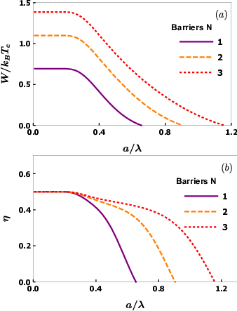
This section studies work and efficiency in the scenario where we insert $N$ barriers symmetrically into the box. The details of the Stirling cycle for this process has been provided in Appendix A.2. We analyse the work and efficiency for multiple barrier insertions as functions of the length of the box and $T_{h}/T_{c}$ , similar to that in Sec. III.2.1, and we use the partition functions Eq. (43) to Eq. (46).

In the low temperature limit, the work for multiple barrier insertion case attains a value of $(T_{h}/T_{c}-1)\ln(N+1)$ , which can be numerically verified from Fig. 9(a). The work, therefore, increases with an increase in the number of barriers.

We explain the work extracted in the low temperature limit due to the degeneracy of the lowest energy level as it is the only energy level which is accessible in this limit. We note that $N+1$ is the degeneracy of the energy levels of the box after symmetric insertion of $N$ barriers. Therefore, the factor $\ln(N+1)$ arising in the work can be attributed to the degeneracy of the ground state energy level. As pointed out earlier, it is the lack of information due to this degeneracy that is converted to work in our degeneracy assisted quantum heat engine. Hence in the low temperature limit, the work is entropic in the sense that it is proportional to the Boltzmann entropy given as $S=k_{B}\ln(N+1)$ . A direct verification of this claim can be stated. If the barrier is inserted in a manner such that no degeneracy is attained, we would expect the low temperature limit of the work obtained to be zero. This is one of the motivations behind the analysis of asymmetric barrier insertion in the next section.

In the low temperature limit, the efficiency turns out to be $1-T_{c}/T_{h}$ , which can be numerically verified from Fig. 9(b). Thus, in the low temperature limit, efficiency is independent of the number of barriers. However, in the high temperature limit, efficiency does depend on the number of barriers. Further, as we increase the number of barriers, work and efficiency become zero at larger values of $a/\lambda$ .

We also plot work and efficiency with respect to $T_{h}/T_{c}$ in Fig. 10 for different number of barriers. We can see that as $T_{h}/T_{c}$ increases, both work and efficiency attain a maximum and then gradually come down to zero for any fixed number of barriers. We also observe that as the number of barriers increases, the maximum value of both work and efficiency increases. Further, with an increase in the number of barriers, the maximum as well as zero shifts to higher values of $T_{h}/T_{c}$ .

III.2.3 Asymmetric insertion of a single barrier

In this section, we examine the work and efficiency for an asymmetric insertion of a barrier in the box, as functions of the length of the box and $T_{h}/T_{c}$ , and we use the partition functions Eq. (49) to Eq. (52). This process divides the box into two parts of lengths $x$ and $y$ with $x+y=2a$ . We provide the details of the Stirling cycle for this case in Appendix A.3. We first study the work $W/k_{B}T_{c}$ as a function of the length of the box $a/\lambda$ for different values of $`d\textrm{'}$ , which we define to be the ratio of the lengths of the two box parts, i.e., $d=x/y$ . The results are shown in Fig. 11. The plots reveal that both work and efficiency attain a maximum at a certain value of $a/\lambda$ . This result is completely different from the symmetric barrier insertion case Fig. 6. Interestingly, the work in the low temperature limit goes to zero as predicted from the $\ln(N+1)$ dependence, (where $N+1$ is the degeneracy of the lowest energy level). The rationale behind this behaviour would be that in the low temperature limit, only the lowest energy level is accessible, which is non-degenerate in the case of asymmetric barrier insertion, and consequently the work reduces to zero.

We now move on to study the work and efficiency dependence on the temperature for different half-lengths of the box $a=\lambda/3$ , $\lambda/4$ , and $\lambda/5$ , where $\lambda=h/\sqrt{2mk_{B}T_{c}}$ is the thermal de Broglie wavelength. The results are shown in Fig. 12. We have set $d=0.95$ in both the plots. We observe that both work and efficiency attain a maximum at a certain specific value of $T_{h}/T_{c}$ . This result is similar compared to the symmetric barrier insertion case Fig. 7; however, the magnitude of work and efficiency decreases in the asymmetric insertion case compared to the symmetric one.

IV Concluding remarks

In this paper, we proposed a degeneracy assisted HO-QSHE in this work and analysed the work and efficiency as functions of the frequency of the harmonic oscillator and the ratio $T_{h}/T_{c}$ of temperatures of the hot and cold thermal baths. We also examined PIB-QSHE in full detail, which was proposed in Thomas et al. 2019. We note that the energy levels are inhomogeneously scaled upon symmetric insertion of a single barrier in harmonic oscillator and particle in a box Gelbwaser-Klimovsky et al. 2018. We showed that efficiency is maximized at certain temperature ratios for both HO-QSHE and PIB-QSHE. However, the work extracted can only be maximized for PIB-QSHE at a certain temperature ratio. It remains an open problem to find out the reason behind this contrasting behaviour. In the low temperature limit, efficiency of both the HO-QSHE and PIB-QSHE approach the Carnot efficiency.

We would like to point out one important distinction between a harmonic oscillator and particle in a box. The two systems differ in the way their specific heat capacity behaves as a function of temperature. This is essentially a consequence of the difference in the structures of the energy levels in a harmonic oscillator and particle in a box. For a one dimensional harmonic oscillator, the heat capacity per particle increases monotonically with temperature and asymptotically reaches $k_{B}$ in the infinite temperature limit. On the other hand, for a one dimensional particle in a box, the heat capacity per particle starts to increase with temperature and attains a maximum value of approximately $9k_{B}/16$ and in the high-temperature limit approaches $k_{B}/2$ from the above Rosenstock 1962. A careful analysis of these facts will provide more insights into the working principle of degeneracy assisted quantum heat engines and might help in resolving the aforementioned problem.

Quantum heat engines have already been realised on several different systems, for instance, quantum dots Josefsson et al. 2018, cold bosonic ions Fialko and Hallwood 2012, optomechanical systems Zhang et al. 2014b, and liquid NMR based platforms Batalhão et al. 2014. The degeneracy assisted quantum heat engine proposed in this work may be practically realised in the near future and our theoretical analysis would be useful in operating the quantum heat engine at optimal conditions.

As we have mentioned earlier that efficiency of quantum heat engines can go beyond the Carnot limit, it would be interesting to see this effect for degeneracy assisted quantum heat engines by considering different type of baths. Another interesting direction is to construct a quantum engine based on entangled states of the harmonic oscillator (an infinite-dimensional system). Entangled quantum heat engines based on two qubit systems Zhang et al. 2007; Thomas and Johal 2011; Yin et al. 2020 (a finite-dimensional system) have already been proposed.

Acknowledgement

A.K. and C.K. thank Narayansami Sathyamurthy for initial discussions on the subject. All the authors thank George Thomas, Narayansami Sathyamurthy, and Upendra Harbola for their invaluable comments on the final version of the draft. We dedicate this work to Prof. N. Sathyamurthy’s forthcoming 70th birthday. C.K. acknowledges the financial support from DST/ICPS/QuST/Theme-1/2019/General Project number Q-68.

Appendix A Particle in a box based quantum Stirling heat engine: background material

In the Appendix, we discuss quantum Stirling heat engine with a particle in a box as the working medium (PIB-QSHE) Thomas et al. 2019. We consider three different scenarios in details: (i) symmetric insertion of a single barrier, (ii) symmetric insertion of multiple barriers, and (iii) asymmetric insertion of a single barrier.

A.1 Symmetric insertion of single barrier

We first consider symmetric insertion of single barrier in a box of length $2a$ .

First step : In the first step, we insert a barrier in the middle of the box, which is coupled to a thermal bath at temperature $T_{h}$ . The insertion of the barrier is done in a quasi-static manner, so that the system is in equilibrium with the thermal bath during the entire process. For the working medium as a particle of mass $m$ confined in a one dimensional box of length $2a$ , the $n^{th}$ energy level is given as

\displaystyle E_{n}=\frac{n^{2}\hbar^{2}\pi^{2}}{2m(2a)^{2}}\quad\text{with}\,n=1,2,3,\dots.

(23)

Therefore, the expression for the partition function $Z_{1}$ can be written as

Z_{(1)}=\sum_{n=1}^{\infty}e^{-\frac{E_{n}}{k_{B}T_{h}}}=\sum_{n=1}^{\infty}e^{-\frac{n^{2}\pi^{2}\hbar^{2}}{2m(2a)^{2}k_{B}T_{h}}}.

(24)

The partition function $Z_{1}$ can also be expressed in terms of Jacobi Theta functions as

Z_{(1)}=\frac{1}{2}\bigg[-1+\Theta_{3}\bigg(0,e^{\frac{\pi^{2}\hbar^{2}}{2m(2a)^{2}k_{B}T_{h}}}\bigg)\bigg],

(25)

where $\Theta_{3}(z,q)$ is defined as

\Theta_{3}(z,q)=1+2\sum_{n=1}^{\infty}q^{n^{2}}cos(2nz).

(26)

The final state obtained after the isothermal process by the quasi-static insertion of the barrier introduces an additional constraint that the probability amplitude of the wave function should be exactly zero in the middle of the box, as well as at the boundaries of the box. Consequently, the wave functions with odd quantum number are ‘raised’ in energy to the next even numbered energy state. Hence, the energy states with even quantum number are now doubly degenerate. The eigenstates of the new system are given as

E_{n}=\frac{(2n)^{2}\pi^{2}\hbar^{2}}{2m(2a)^{2}}\quad\text{with}\,n=1,2,3,\dots.

(27)

Thus, the partition function can be expressed as

Z_{(2)}=\sum_{n=1}^{\infty}2e^{-\frac{(2n)^{2}\pi^{2}\hbar^{2}}{2m(2a)^{2}k_{B}T_{h}}}=2Z^{a}_{T_{h}},

(28)

where,

Z^{a}_{T_{h}}=\sum_{n=1}^{\infty}e^{-\frac{n^{2}\pi^{2}\hbar^{2}}{2ma^{2}k_{B}T_{h}}},

is the partition function of a particle in a box of length $a$ attached to a bath at temperature $T_{h}$ . In terms of the Jacobi Theta function, the partition function $Z_{(2)}$ of the final state is obtained as

Z_{(2)}=2\bigg\{\frac{1}{2}\bigg[-1+\Theta_{3}\bigg(0,e^{\frac{\pi^{2}\hbar^{2}}{2ma^{2}k_{B}T_{h}}}\bigg)\bigg]\bigg\}.

(29)

The heat absorbed in the process is

Q_{12}=U_{(2)}-U_{(1)}+k_{B}T_{h}\ln Z_{(2)}-k_{B}T_{h}\ln Z_{(1)}.

(30)

The change in internal energy is

\Delta U_{12}=U_{(2)}-U_{(1)}=-\frac{\partial}{\partial\beta_{h}}[\ln Z_{(2)}-\ln Z_{(1)}].

(31)

Thus, the work done in the process can be directly written as following by the first law of thermodynamics:

W_{12}=Q_{12}-\Delta U_{12}=k_{B}T_{h}\ln Z_{(2)}-k_{B}T_{h}\ln Z_{(1)}.

(32)

Second step : In this step, the system is attached with a cold bath at temperature $T_{c}$ after disconnecting it from the hot bath at temperature $T_{h}$ . This results in lowering the temperature of the system from $T_{h}$ to $T_{c}$ .

The partition function of the final state can be written as

Z_{(3)}=\sum_{n=1}^{\infty}2e^{-\frac{n^{2}\pi^{2}\hbar^{2}}{2ma^{2}k_{B}T_{c}}}.

(33)

In terms of the Jacobi Theta function, the expression turns out to be:

Z_{(3)}=\bigg[-1+\Theta_{3}\bigg(0,e^{\frac{\pi^{2}\hbar^{2}}{2ma^{2}k_{B}T_{c}}}\bigg)\bigg].

(34)

Since no mechanical work is done ( $W_{23}=0$ ), the heat lost is equal to the change in internal energy:

Q_{23}=U_{(3)}-U_{(2)}=-\frac{\partial\ln Z_{(3)}}{\partial\beta_{c}}+\frac{\partial\ln Z_{(2)}}{\partial\beta_{h}}.

(35)

Third step : In the next step, the barrier is lifted in a quasi-static manner such that the system is in equilibrium with the thermal bath at temperature $T_{c}$ during the whole process. This brings the system to the same energy level structure as that of the initial state $(1)$ . The partition function of the final state is given as

	$\displaystyle Z_{(4)}$	$\displaystyle=$	$\displaystyle\sum_{n=1}^{\infty}e^{-\frac{n^{2}\pi^{2}\hbar^{2}}{2m(2a)^{2}k_{B}T_{c}}},$		(36)
		$\displaystyle=$	$\displaystyle\frac{1}{2}\bigg[-1+\Theta_{3}\bigg(0,e^{\frac{\pi^{2}\hbar^{2}}{2m(2a)^{2}k_{B}T_{c}}}\bigg)\bigg].$		(36)

The heat lost at end of the process is obtained in terms of the partition functions as

Q_{34}=U_{(4)}-U_{(3)}+k_{B}T_{c}\ln Z_{(4)}-k_{B}T_{c}\ln Z_{(3)}.

(37)

The work done in the process is

W_{34}=Q_{34}-\Delta U_{34}=k_{B}T_{c}\ln Z_{(4)}-k_{B}T_{c}\ln Z_{(3)},

(38)

where $\Delta U_{34}$ is $U_{(4)}-U_{(3)}$ .

Fourth step : In the final step, the system is connected to a thermal bath at temperature $T_{h}>T_{c}$ after disconnecting it from the thermal bath at temperature $T_{c}$ . The temperature of the system is raised from $T_{c}$ to $T_{h}$ during this process and the system is restored to the initial state $(1)$ . The heat absorbed by the system is given as

Q_{41}=-\frac{\partial\ln Z_{(1)}}{\partial\beta_{h}}+\frac{\partial\ln Z_{(4)}}{\partial\beta_{c}}.

(39)

These four processes comprise one complete cycle of the heat engine. The net work done by the heat engine in one complete cycle is given as

	$\displaystyle W_{\textrm{net}}$	$\displaystyle=$	$\displaystyle W_{12}+W_{34},$		(40)
		$\displaystyle=$	$\displaystyle k_{B}T_{c}\ln\frac{Z_{(4)}}{Z_{(3)}}+k_{B}T_{h}\ln\frac{Z_{(2)}}{Z_{(1)}}.$		(40)

Further, the total heat absorbed by the system can be written as

Q_{\textrm{in}}=Q_{12}+Q_{41}.

(41)

The efficiency $\eta$ for the cycle is given as:

\eta=\frac{W_{\textrm{net}}}{Q_{\textrm{in}}}=1+\frac{Q_{23}+Q_{34}}{Q_{12}+Q_{41}}.

(42)

More details about PIB-QSHE are available in Thomas et al. 2019.

A.2 Symmetric insertion of multiple barriers

We now generalize the PIB-QSHE to the scenario where we insert $N$ barriers symmetrically into the box. To understand the changes in the energy levels, let us consider the insertion of two barriers symmetrically into the box of length $2a$ . This divides the box into three equal parts, each of length $2a/3$ . The energy levels which have nodes falling on the barrier positions remain unchanged, while the other energy levels shift up to the nearest unchanged energy level. This renders an energy level structure, where each energy state is three-fold degenerate. Similarly, for symmetric insertion of $N$ barriers, we obtain an energy level structure with $N$ -fold degeneracy.

The expression for partition functions at various four stages of the Stirling cycle, as mentioned in Appendix A.1, for symmetric insertion of $N$ barriers is given as follows:

	$\displaystyle Z_{(1)}$	$\displaystyle=$	$\displaystyle\sum_{n=1}^{\infty}e^{-\frac{n^{2}\pi^{2}\hbar^{2}}{2m(2a)^{2}k_{B}T_{h}}},$		(43)
		$\displaystyle=$	$\displaystyle\frac{1}{2}\bigg[-1+\Theta_{3}\bigg(0,e^{\frac{\pi^{2}\hbar^{2}}{2m(2a)^{2}k_{B}T_{h}}}\bigg)\bigg].$		(43)

	$\displaystyle Z_{(2)}$	$\displaystyle=$	$\displaystyle N\sum_{n=1}^{\infty}e^{-\frac{n^{2}\pi^{2}\hbar^{2}}{2m(2a/N)^{2}k_{B}T_{h}}},$		(44)
		$\displaystyle=$	$\displaystyle N\bigg\{\frac{1}{2}\bigg[-1+\Theta_{3}\bigg(0,e^{\frac{\pi^{2}\hbar^{2}}{2m(2a/N)^{2}k_{B}T_{h}}}\bigg)\bigg]\bigg\}.$		(44)

	$\displaystyle Z_{(3)}$	$\displaystyle=$	$\displaystyle N\sum_{n=1}^{\infty}e^{-\frac{n^{2}\pi^{2}\hbar^{2}}{2m(2a/N)^{2}k_{B}T_{c}}},$		(45)
		$\displaystyle=$	$\displaystyle N\bigg\{\frac{1}{2}\bigg[-1+\Theta_{3}\bigg(0,e^{\frac{\pi^{2}\hbar^{2}}{2m(2a/N)^{2}k_{B}T_{c}}}\bigg)\bigg]\bigg\}.$		(45)

	$\displaystyle Z_{(4)}$	$\displaystyle=$	$\displaystyle\sum_{n=1}^{\infty}e^{-\frac{n^{2}\pi^{2}\hbar^{2}}{2m(2a)^{2}k_{B}T_{c}}},$		(46)
		$\displaystyle=$	$\displaystyle\frac{1}{2}\bigg[-1+\Theta_{3}\bigg(0,e^{\frac{\pi^{2}\hbar^{2}}{2m(2a)^{2}k_{B}T_{c}}}\bigg)\bigg].$		(46)

Using these partition functions, we can write the corresponding work (40) and efficiency equation (42).

A.3 Asymmetric insertion of single barrier

We insert a barrier asymmetrically into the box such that it is divided into two parts of length $x$ and $y$ with $x+y=2a$ .

The energy eigenstates for a particle in a box of length $x$ and $y$ is given as follows:

\displaystyle E_{i}=\sum_{i=1}^{\infty}e^{-\frac{i^{2}\pi^{2}\hbar^{2}}{2mx^{2}}}\quad\text{with}\,i=1,2,3,\dots,

(47)

and

\displaystyle E_{i}^{\prime}=\sum_{i=1}^{\infty}e^{-\frac{{i^{\prime}}^{2}\pi^{2}\hbar^{2}}{2my^{2}}}\quad\text{with}\,i^{\prime}=1,2,3,\dots.

(48)

The energy level structure is a collection of all these energy eigenstates corresponding to the two boxes. Therefore, the partition function after the asymmetric insertion of barrier is the sum of Boltzmann factor over the whole energy level structure, i.e., all the energy eigenstates corresponding to the two boxes.

The expression for various partition functions at the four stages of the Stirling cycle, as discussed in Appendix A.1, for asymmetric insertion of a single barrier is given as follows:

	$\displaystyle Z_{(1)}$	$\displaystyle=$	$\displaystyle\sum_{n=1}^{\infty}e^{-\frac{n^{2}\pi^{2}\hbar^{2}}{2m(2a)^{2}k_{B}T_{h}}},$		(49)
		$\displaystyle=$	$\displaystyle\frac{1}{2}\bigg[-1+\Theta_{3}\bigg(0,e^{\frac{\pi^{2}\hbar^{2}}{2m(2a)^{2}k_{B}T_{h}}}\bigg)\bigg].$		(49)

$\displaystyle Z_{(2)}$	$\displaystyle=$	$\displaystyle\sum_{n=1}^{\infty}e^{-\frac{n^{2}\pi^{2}\hbar^{2}}{2mx^{2}k_{B}T_{h}}}+\sum_{n=1}^{\infty}e^{-\frac{n^{2}\pi^{2}\hbar^{2}}{2my^{2}k_{B}T_{h}}},$	(50)
	$\displaystyle=$	$\displaystyle\frac{1}{2}\bigg[-1+\Theta_{3}\bigg(0,e^{\frac{\pi^{2}\hbar^{2}}{2mx^{2}k_{B}T_{h}}}\bigg)\bigg]$
		$\displaystyle+\frac{1}{2}\bigg[-1+\Theta_{3}\bigg(0,e^{\frac{\pi^{2}\hbar^{2}}{2my^{2}k_{B}T_{h}}}\bigg)\bigg].$

$\displaystyle Z_{(3)}$	$\displaystyle=$	$\displaystyle\sum_{n=1}^{\infty}e^{-\frac{n^{2}\pi^{2}\hbar^{2}}{2mx^{2}k_{B}T_{c}}}+\sum_{n=1}^{\infty}e^{-\frac{n^{2}\pi^{2}\hbar^{2}}{2my^{2}k_{B}T_{c}}},$	(51)
	$\displaystyle=$	$\displaystyle\frac{1}{2}\bigg[-1+\Theta_{3}\bigg(0,e^{\frac{\pi^{2}\hbar^{2}}{2mx^{2}k_{B}T_{c}}}\bigg)\bigg]$
		$\displaystyle+\frac{1}{2}\bigg[-1+\Theta_{3}\bigg(0,e^{\frac{\pi^{2}\hbar^{2}}{2my^{2}k_{B}T_{c}}}\bigg)\bigg].$

	$\displaystyle Z_{(4)}$	$\displaystyle=$	$\displaystyle\sum_{n=1}^{\infty}e^{-\frac{n^{2}\pi^{2}\hbar^{2}}{2m(2a)^{2}k_{B}T_{c}}},$		(52)
		$\displaystyle=$	$\displaystyle\frac{1}{2}\bigg[-1+\Theta_{3}\bigg(0,e^{\frac{\pi^{2}\hbar^{2}}{2m(2a)^{2}k_{B}T_{c}}}\bigg)\bigg].$		(52)

The above partition functions can be utilised to write the work (40) and efficiency equation (42). We note that for $x=y$ , the situation becomes the same as the symmetric insertion of a single barrier case, which has been dealt with in Appendix A.1.

References

Carnot (2005) S. Carnot, Reflections on the motive power of fire: and other papers on the second law of thermodynamics, Dover Books on Physics (Dover, Mineola, NY, 2005).
Maxwell (1860) J. C. Maxwell, Philosophical Magazine 1, 377 (1860).
Boltzmann (1872) L. Boltzmann, Ann. Phys.(Leipzig) 57, 773 (1872).
Klaers et al. (2017) J. Klaers, S. Faelt, A. Imamoglu, and E. Togan, Phys. Rev. X 7, 031044 (2017).
Peterson et al. (2019) J. P. S. Peterson, T. B. Batalhão, M. Herrera, A. M. Souza, R. S. Sarthour, I. S. Oliveira, and R. M. Serra, Phys. Rev. Lett. 123, 240601 (2019).
Vinjanampathy and Anders (2016) S. Vinjanampathy and J. Anders, Contemporary Physics 57, 545 (2016).
Binder et al. (2019) F. Binder, L. Correa, C. Gogolin, J. Anders, and G. Adesso, Thermodynamics in the Quantum Regime: Fundamental Aspects and New Directions, Fundamental Theories of Physics (Springer International Publishing, 2019).
Bhattacharjee and Dutta (2020) S. Bhattacharjee and A. Dutta, arXiv 2008.07889 (2020).
Scovil and Schulz-DuBois (1959) H. E. D. Scovil and E. O. Schulz-DuBois, Phys. Rev. Lett. 2, 262 (1959).
Quan et al. (2007) H. T. Quan, Y.-x. Liu, C. P. Sun, and F. Nori, Phys. Rev. E 76, 031105 (2007).
Günter (2015) M. Günter, Quantum thermodynamic processes: energy and information flow at the nanoscale (Pan Stanford Publ., 2015).
Quan (2009) H. T. Quan, Phys. Rev. E 79, 041129 (2009).
Chen et al. (2020) L. Chen, X. Liu, F. Wu, S. Xia, and H. Feng, Physica A: Statistical Mechanics and its Applications 537, 122597 (2020).
Tajima and Hayashi (2017) H. Tajima and M. Hayashi, Phys. Rev. E 96, 012128 (2017).
Wang et al. (2009) H. Wang, S. Liu, and J. He, Applied Thermal Engineering 29, 706 (2009).
Stefanatos (2014) D. Stefanatos, Phys. Rev. E 90, 012119 (2014).
Thomas et al. (2019) G. Thomas, D. Das, and S. Ghosh, Phys. Rev. E 100, 012123 (2019).
Wu et al. (2006) F. Wu, L. Chen, F. Sun, C. Wu, and Q. Li, Phys. Rev. E 73, 016103 (2006).
Dong et al. (2013) C. D. Dong, G. Lefkidis, and W. Hübner, Phys. Rev. B 88, 214421 (2013).
Zhang et al. (2014a) X. Y. Zhang, X. L. Huang, and X. X. Yi, Journal of Physics A: Mathematical and Theoretical 47, 455002 (2014a).
Scully et al. (2003) M. O. Scully, M. S. Zubairy, G. S. Agarwal, and H. Walther, Science 299, 862 (2003).
Quan et al. (2006) H. T. Quan, P. Zhang, and C. P. Sun, Phys. Rev. E 73, 036122 (2006).
Huang et al. (2012) X. L. Huang, T. Wang, and X. X. Yi, Phys. Rev. E 86, 051105 (2012).
Roßnagel et al. (2014) J. Roßnagel, O. Abah, F. Schmidt-Kaler, K. Singer, and E. Lutz, Phys. Rev. Lett. 112, 030602 (2014).
Niedenzu et al. (2018) W. Niedenzu, V. Mukherjee, A. Ghosh, A. G. Kofman, and G. Kurizki, Nature Communications 9, 165 (2018).
Wang et al. (2019) J. Wang, J. He, and Y. Ma, Phys. Rev. E 100, 052126 (2019).
Dillenschneider and Lutz (2009) R. Dillenschneider and E. Lutz, EPL (Europhysics Letters) 88, 50003 (2009).
Geva and Kosloff (1992) E. Geva and R. Kosloff, The Journal of Chemical Physics 96, 3054 (1992).
Harbola et al. (2012) U. Harbola, S. Rahav, and S. Mukamel, EPL (Europhysics Letters) 99, 50005 (2012).
Rahav et al. (2012) S. Rahav, U. Harbola, and S. Mukamel, Phys. Rev. A 86, 043843 (2012).
Hamedani Raja et al. (2020) S. Hamedani Raja, S. Maniscalco, G.-S. Paraoanu, J. P. Pekola, and N. Lo Gullo, arXiv e-prints , arXiv:2009.10038 (2020), arXiv:2009.10038 [quant-ph] .
Su et al. (2018) S. Su, Y. Zhang, G. Su, and J. Chen, Physics Letters A 382, 2108 (2018).
Lin and Chen (2003a) B. Lin and J. Chen, Phys. Rev. E 67, 046105 (2003a).
Lin and Chen (2003b) B. Lin and J. Chen, Journal of Applied Physics 94, 6185 (2003b).
Insinga et al. (2016) A. Insinga, B. Andresen, and P. Salamon, Phys. Rev. E 94, 012119 (2016).
Kosloff and Rezek (2017) R. Kosloff and Y. Rezek, Entropy 19, 136 (2017).
Gelbwaser-Klimovsky et al. (2018) D. Gelbwaser-Klimovsky, A. Bylinskii, D. Gangloff, R. Islam, A. Aspuru-Guzik, and V. Vuletic, Phys. Rev. Lett. 120, 170601 (2018).
Sakurai and Napolitano (2017) J. J. Sakurai and J. Napolitano, Modern Quantum Mechanics, 2nd ed. (Cambridge University Press, 2017).
(39) Any generic potential can be Taylor expanded near equilibrium at $x=x_{0}$ as $U(x)=U(x_{0})+(x-x_{0})\frac{dU}{dx}|_{x=x_{0}}+\frac{(x-x_{0})^{2}}{2!}\frac{d^{2}U}{dx^{2}}|_{x=x_{0}}+\cdots$ . Since at equilibrium, $\frac{dU}{dx}|_{x=x_{0}}$ is zero and usually the physics is not affected by the constant potential $U(x_{0})$ . Therefore, we can approximate the generic potential as harmonic oscillator, $U(x)\approx\frac{(x-x_{0})^{2}}{2!}\frac{d^{2}U}{dx^{2}}|_{x=x_{0}}$ , for small oscillations around equilibrium.
Scharf et al. (2020) B. Scharf, A. Braggio, E. Strambini, F. Giazotto, and E. M. Hankiewicz, Communications Physics 3, 198 (2020).
Barontini and Paternostro (2019) G. Barontini and M. Paternostro, New Journal of Physics 21, 063019 (2019).
Paraoanu et al. (2001) G.-S. Paraoanu, S. Kohler, F. Sols, and A. J. Leggett, Journal of Physics B: Atomic, Molecular and Optical Physics 34, 4689 (2001).
Weedbrook et al. (2012) C. Weedbrook, S. Pirandola, R. García-Patrón, N. J. Cerf, T. C. Ralph, J. H. Shapiro, and S. Lloyd, Rev. Mod. Phys. 84, 621 (2012).
Sattler (2010) K. D. Sattler, Handbook of Nanophysics: Nanotubes and Nanowires (CRC Press, 2010).
Griffiths (2005) D. J. Griffiths, Introduction to quantum mechanics, 2nd ed. (Pearson Prentice Hall, 2005) pp. 86–87.
Sørdal and Bergli (2019) V. B. Sørdal and J. Bergli, Phys. Rev. A 99, 022121 (2019).
Li et al. (2012) H. Li, J. Zou, J.-G. Li, B. Shao, and L.-A. Wu, Annals of Physics 327, 2955 (2012).
Rosenstock (1962) H. B. Rosenstock, American Journal of Physics 30, 38 (1962).
Josefsson et al. (2018) M. Josefsson, A. Svilans, A. M. Burke, E. A. Hoffmann, S. Fahlvik, C. Thelander, M. Leijnse, and H. Linke, Nature Nanotechnology 13, 920 (2018).
Fialko and Hallwood (2012) O. Fialko and D. W. Hallwood, Phys. Rev. Lett. 108, 085303 (2012).
Zhang et al. (2014b) K. Zhang, F. Bariani, and P. Meystre, Phys. Rev. Lett. 112, 150602 (2014b).
Batalhão et al. (2014) T. B. Batalhão, A. M. Souza, L. Mazzola, R. Auccaise, R. S. Sarthour, I. S. Oliveira, J. Goold, G. De Chiara, M. Paternostro, and R. M. Serra, Phys. Rev. Lett. 113, 140601 (2014).
Zhang et al. (2007) T. Zhang, W.-T. Liu, P.-X. Chen, and C.-Z. Li, Phys. Rev. A 75, 062102 (2007).
Thomas and Johal (2011) G. Thomas and R. S. Johal, Phys. Rev. E 83, 031135 (2011).
Yin et al. (2020) Y. Yin, L. Chen, F. Wu, and Y. Ge, Physica A: Statistical Mechanics and its Applications 547, 123856 (2020).