Sub-Linear Memory: How to Make Performers SLiM

We commence by defining exponential self-attention (Vaswani et al. 2017), a key component of the Transformer. Consider a sequence scale $l\in\{1,\dots,L\}$ and three matrices: queries $\mathbf{Q}\in\mathbb{R}^{L\times d}$, keys $\mathbf{K}\in\mathbb{R}^{L\times d}$ and values $\mathbf{V}\in\mathbb{R}^{L\times d}$. Then exponential self-attention is defined as a functional producing $\mathbf{Y}=\mathrm{Att}^{exp}(\mathbf{Q},\mathbf{K},\mathbf{V})\in\mathbb{R}^{L\times d}$,

where by $\mathbf{Z}_{l}\in\mathbb{R}^{d_{2}\times\dots}$ we denote slice $\mathbf{Z}_{l,:,\dots,:}$ of a tensor $\mathbf{Z}\in\mathbb{R}^{d_{1}\times d_{2}\times\dots}$. Mapping (1) is designed as a differentiable dictionary, where output at index $l$ is a weighted average over value vectors $\mathbf{V}_{:l}$. For needs of autoregressive generative modelling, when each element depends only on previous elements of the sequence (Vaswani et al. 2017), $\mathbf{Y}_{l}$ only depends on inputs at indices $\{1,\dots,l\}$. Self-attention of type (1) is a key contributor to state-of-the-art results in many applications. However, its running time and memory scale as $O(L^{2})$. This prevents applicability of exponential self-attention to sequences of big length $L\gg d$. Hence, linear self-attention methods were proposed (Katharopoulos et al. 2020; Choromanski et al. 2020; Shen et al. 2018; Li et al. 2020), where the exponent is substituted by a Euclidean inner-product. This is defined as a functional $\mathbf{Y}=\mathrm{Att}^{lin}(\mathbf{Q},\mathbf{K},\mathbf{V})\in\mathbb{R}^{L\times d}$, where

where “$\times$” denotes a matrix-matrix or matrix-vector product and $g:\mathbb{R}^{d}\to\mathbb{R}_{+}^{M}$ is a mapping into a vector with positive elements. The positivity of the result is to guarantee that the division in (2) is well-defined and stable. In practice, $M$ is chosen to be much smaller than $L$. $g(\cdot)$ can be chosen as a simple elementwise mapping (so that $d=M$). Choromanski et al. 2020 propose a randomized form of $g(\cdot)$, which is an unbiased approximation to exponential self-attention (1). The second transition in (2), which is due to associativity of matrix multiplication, suggests an algorithm to compute linear self-attention efficiently in subqudratic time.

For a series of tensors $\mathbf{Z}^{(1)},\dots,\mathbf{Z}^{(n)}$ of the same shape, by $\mathbf{Z}=(\mathbf{Z}^{(i)})_{i=1}^{n}$ we understand a tensor such that for all $1\leq i\leq n$ $\mathbf{Z}_{i,:,\dots,:}=\mathbf{Z}^{(i)}$. By $\mathbf{R}\in\mathbb{R}^{L\times d\times M}$, $\mathbf{S}\in\mathbb{R}^{L\times M}$ denote a tensor and a matrix such that

where $\mathrm{PS}(\mathbf{Z})=(\sum_{i^{\prime}=1}^{i}\mathbf{Z}_{i^{\prime}})_{i=1}^{n}$ is an operator taking a prefix sum (or a cumulative sum) along the first dimension of the input tensor $\mathbf{Z}$. Next, compute

Depending on the prefix-sum algorithm used in (3), we can obtain different complexity estimates for linear self-attention. Katharopoulos et al. 2020 propose to iterate through $l=1,\dots,L$ maintaining only current $\mathbf{R}_{l},\mathbf{S}_{l}$, and compute and store the result $\widetilde{\mathbf{Y}}_{l}$. This way, tensors $\mathbf{R},\mathrm{PS}(\mathbf{R})\in\mathbb{R}^{L\times d\times M}$ are not stored in memory, resulting in $O(L)$ time complexity and $O(L(d+M)+dM)$ memory complexity. Katharopoulos et al. 2020 also propose a similar iterative scheme for computing gradients through (3-4); see Appendix B for a detailed discussion.

Alternatively, Choromanski et al. 2020 employ a parallel prefix-sum algorithm (Ladner & Fischer 1980; Vishkin 2010), which, for a tensor $\mathbf{Z}\in\mathbb{R}^{L\times\dots}$, finds $\mathrm{PS}(\mathbf{Z})$ in $O(\log L)$ parallel time and $O(L)$ memory. Applying this algorithm for computing $\mathrm{PS}(\mathbf{R})$, $\mathrm{PS}(\mathbf{S})$ and then computing (4) results in only $O(\log L)$ parallel time complexity and $O(LdM)$ memory consumption.

In this subsection we outline a Transformer architecture which is used for autoregressive language modelling (Parmar et al. 2018). We focus on language modelling: first, to simplify notation, while our subsequent derivations are applicable in broader setups; second, language models are a crucial class of architectures because they were shown to act as few-shot learners, e.g. the seminal GPT-2 (Radford et al. 2019) and GPT-3 (Brown et al. 2020).

Let $\mathbf{p}\in\Sigma^{L}$ be an input sequence of length $L$, where $\Sigma$ is a finite alphabet. By $\mathrm{emb}(\mathbf{p}_{l},l)\in\mathbb{R}^{d_{model}}$, $1\leq l\leq L$, denote a linear combination of the $\mathbf{p}_{l}$ token’s learned embedding and positional embedding of $l$’s position (sinusoids with different frequencies, as in (Vaswani et al. 2017)). Then Transformer is defined as a parametrized mapping from $\mathbf{X}^{(0)}=(\mathrm{emb}(\mathbf{p}_{l},l))_{l=1}^{L}\in\mathbb{R}^{L\times d_{model}}$ into $\mathbf{X}^{(out)}\in\mathbb{R}^{L\times|\Sigma|}$ through a sequence of hidden representations $\mathbf{X}^{(1)},\dots,\mathbf{X}^{(s)}\in\mathbb{R}^{L\times d_{model}}$. More formally, $\mathbf{X}^{(out)}=\mathbf{X}^{(s)}\mathbf{W}^{(out)}+\mathbf{b}^{(out)}$ and for each $1\leq r\leq s$:

Here $\mathrm{Att}$ is either $\mathrm{Att}^{exp}$ or $\mathrm{Att}^{lin}$ and $k$ is the number of attention heads ($d_{model}=kd$). $\mathbf{W}^{(out)}\in\mathbb{R}^{d_{model}\times|\Sigma|}$, $\mathbf{b}^{(out)}\in\mathbb{R}^{1\times|\Sigma|}$, $\mathbf{W}^{(1)}\in\mathbb{R}^{d_{model}\times d_{ff}}$, $\mathbf{b}^{(1)}\in\mathbb{R}^{1\times d_{ff}}$, $\mathbf{W}^{(2)}\in\mathbb{R}^{d_{ff}\times d_{model}}$, $\mathbf{b}^{(2)}\in\mathbb{R}^{1\times d_{model}}$, $\mathbf{W}^{(j)}_{Q},\mathbf{W}^{(j)}_{K},\mathbf{W}^{(j)}_{V}\in\mathbb{R}^{d_{model}\times d}$ are trainable parameters (separate for each instance of $\mathrm{MultiHead}\text{-}\mathrm{Att}$, $\mathrm{FFN}$), “$+$” is broadcasted rowwise when biases are added and $\mathrm{LN}$ is layer normalization (Ba et al. 2016), which is applied rowwise and depends on additional trainable parameters. $\mathrm{GeLU}$ denotes Gaussian error Linear Unit (Hendrycks & Gimpel 2016), which is applied elementwise. We refer to the Transformer (5-9) with linear self-attention $\mathrm{Att}^{lin}$ as Performer.

For each $1\leq l\leq L-1$, $\mathbf{X}^{(out)}_{l}$ denotes predicted logits of the probability distribution over the next token $\mathbf{p}_{l+1}$. Let $\mathcal{L}_{l}(\mathbf{X}^{(out)}_{l})$ denote a cross-entropy loss with respect to $\mathbf{p}_{l+1}$, or zero when $l=L$. The minimized loss is defined as

The Transformer configuration (5-9) can be slightly changed in the literature: different $\mathrm{LN}(\cdot)$ placement, $\mathrm{GeLU}$ replaced with $\mathrm{ReLU}$, etc. The discussed variant (5-9) corresponds to GPT-2. We consider this configuration for simplicity and use it in experiments. However, as we further show, our findings can be easily extended to other modifications.

In this section we consider Performer: the Transformer defined by (5-9) with $\mathrm{Att}=\mathrm{Att}^{lin}$. In light of the definition (5-9) and the algorithm for linear self-attention evaluation (3-4), the sequence of computations $\mathbf{X}^{(0)}\to\mathbf{X}^{(1)}\to\dots\to\mathbf{X}^{(s)}$ can be rewritten in the following compact form, which is more convenient for our subsequent analysis. For each $1\leq r\leq s$,

Here $\theta\in\mathbb{R}^{n_{param}}$ is a set of all trainable parameters, $\mathbf{T}^{(r-1)},\mathbf{U}^{(r-1)}\in\mathbf{R}^{L\times D_{1}}$ and $\mathbf{\Gamma}^{(r-1)}\in\mathbf{R}^{L\times D_{2}}$ are the following matrices (see Figure 1a for an illustration):

• •

  $\mathbf{T}^{(r-1)}$ is a matrix of intermediate representations which are passed into the prefix-sum operator. That is, for each $1\leq l\leq L$, $\mathbf{T}^{(r-1)}_{l}$ is a concatenation of $g(\mathbf{K}_{l})$ and flattened $\mathbf{V}_{l}\times g(\mathbf{K}_{l})^{\top}$ for all attention heads computed at the $r$th step (Equations 8 and 3). Consequently, $D_{1}=M(d+1)k$.

• •

  For each $1\leq l\leq L$, $\mathbf{U}^{(r-1)}_{l}$ is a concatenation of all corresponding $\mathbf{S}_{l}$ and flattened $\mathbf{R}_{l}$ – results of the prefix-sum operation (Equation 3) inside each self-attention head (Equation 8).

• •

  $\mathbf{\Gamma}^{(r-1)}$ is a matrix of representations which skip the prefix-sum operation. For each $1\leq l\leq L$, $\mathbf{\Gamma}^{(r-1)}_{l}$ is a concatenation of $\mathbf{X}^{(r-1)}_{l}$ and $g(\mathbf{Q}^{(j)}_{l})=g(\overline{\mathbf{X}}\mathbf{W}_{Q}^{(j)})$ – query vectors for each attention head $1\leq j\leq k$ (Equations 8 and 4). Therefore, $D_{2}=Mk+d_{model}$.

$F^{(r)}$ and $G^{(r)}$ are functionals parametrized by $\theta$. That is, they take subsets of $\theta$ corresponding to $r$th layer weights (Equations 5-9). $F^{(r)}$ is responsible for constructing $\mathbf{T}^{(r-1)}$ and $\mathbf{\Gamma}^{(r-1)}$ – representations preceding prefix-sum computation, while $G^{(r)}$ finalizes $\mathrm{MultiHead}\text{-}\mathrm{Att}$ computation (7) and includes the feed-forward block (9).

Importantly, $F^{(r)}$ and $G^{(r)}$ are applied rowwise, i.e. (11, 13) can be rewritten as

Hence, the only place where the information is propagated across the sequence dimension is the prefix-sum operation (12).

The representation (11-13) encapsulates architecture details of the Transformer inside $\{F^{(1)},G^{(1)},\dots,F^{(s)},G^{(s)}\}$. In fact, the representation (11-13) holds for various possible modifications of the specification (5-9), proposed in the literature. This includes, but is not limited by the different positioning of layer normalization (Xiong et al. 2020; Vaswani et al. 2017), adding a stabilizing gating mechanism (Parisotto et al. 2019), weight sharing across layers (Lan et al. 2020) or reversible Transformer layers (Kitaev et al. 2020). Therefore, we further analyse the generic, compact notation (11-13) together with the autoregressive loss formulation (10).

Suppose the memory budget is not enough to perform a complete forward pass through Performer (Equations 11-13 for $r=1,\dots,s$), because the input sequence length $L$ is too big. We show that instead we can emulate the full forward computation under the memory needed for a forward pass through the input of length $C\leq L$, plus a small addition. $1\leq C\leq L$ is arbitrary and user-defined.

Split each matrix $\mathbf{X}^{(r)},\mathbf{T}^{(r)},\mathbf{\Gamma}^{(r)},\mathbf{U}^{(r)}$, into $N$ slices of size at most $C$ along the vertical axis ($N=\lceil L/C\rceil$): for each $\forall 1\leq n\leq N$,

where $A_{n}=(n-1)C$ and by $B_{n}$, $1\leq n\leq N$, we denote the size of $n$th slice: $B_{u}=C$ for $u<N$, $B_{N}\leq C$. Based on (11-13), we conclude that for each $1\leq n\leq N$ and $1\leq r\leq s$ the following recurrence holds:

Here $\mathbf{1}_{B_{n}}\in\mathbb{R}^{B_{n}}$ is a vector of $B_{n}$ ones and we denote $\mathbf{U}^{(r-1,0)}_{B_{0}}=\mathbf{0}_{D_{1}}$ (a vector of $D_{1}$ zeros).

Now, instead of iterating over $r=1,\dots s$ and computing (11-13) for the whole sequence at once, we first iterate over $n=1,\dots,N$ and then iterate over $r=1,\dots,s$ in a nested loop to compute (16-18). As can be deduced from the (16-18), we only need to maintain the current value of $(\mathbf{U}^{(r-1,n-1)}_{B_{n-1}})_{r=1}^{s}\in\mathbb{R}^{s\times D_{1}}$ in the outer iteration over $n$.

Denote $\mathcal{B}^{(n)}=(\mathbf{U}^{(r-1,n)}_{B_{n}})_{r=1}^{s}\in\mathbb{R}^{s\times D_{1}}$, $0\leq n\leq N$. The memory-efficient algorithm for the forward pass is as follows. First, initialize $\mathcal{L}=0$ and $\mathcal{B}^{(0)}=\mathbf{0}_{r\times D_{1}}$. Then, iterate over $n=1,\dots,N$ and maintain the current value of $\mathcal{B}^{(n-1)}$. During each iteration, compute $\mathbf{X}^{(0,n)}=(\mathrm{emb}(\mathbf{p}_{A_{n}+l},A_{n}+l))_{l=1}^{B_{n}}$. Then iterate over $r=1,\dots,s$, where compute (16-18) and update $\mathcal{B}^{(n)}_{r}=\mathbf{U}^{(r-1,n)}_{B_{n}}$. Finally, compute $\mathbf{X}^{(out,n)}=\mathbf{X}^{(s,n)}\mathbf{W}^{(out)}+\mathbf{b}^{(out)}$ and update $\mathcal{L}\,+\!\!=\mathcal{L}^{(n)}(\mathbf{X}^{(out,n)})$, where we denote

By the end of the iteration over $n$, the correct loss value (10) is computed. As a result, the forward pass takes $O(L)$ serial time or $O((L/C)\log C)$ parallel time and consumes only $O(C)$ memory. This is in addition to the input sequence $\mathbf{p}\in\Sigma^{L}$ storage, which is $O(L)$ in principle, however the constant is negligibly small. For instance, if $\mathbf{p}$ is a flattened image or an ASCII text string, then it occupies precisely $L$ bytes in memory. The $\log C$ term in the parallel time complexity is due to the parallel prefix-sum algorithm taking logarithmic time, as discussed in Subsection 2.1.

The goal of a backward pass is to compute gradient $\nabla_{\theta}\mathcal{L}$ of the loss function with respect to parameters $\theta$. One can just perform automatic differentiation (Griewank & Walther 2008) (implemented in Tensorflow (Abadi et al. 2015) and Pytorch (Paszke et al. 2017)) through the computation graph induced by the memory-efficient forward pass algorithm from Subsection 3.2. However, such backward pass would need to store all intermediate tensors produced during the forward pass, resulting in $O(L)$ memory complexity as a function of $L$ and $C$. Instead, we propose a back-propagation algorithm which has the same time and memory complexity as the efficient forward pass.

Let $\theta^{(1)}=\dots=\theta^{(N)}=\theta$ be results of a symbolic “identity operation” performed on $\theta$, so that for all $1\leq n\leq N$, $\theta^{(n)}$ is used instead of $\theta$ in (16-18). Then the total gradient of $\theta$ has the form $\nabla_{\theta}\mathcal{L}=\nabla_{\theta^{(1)}}\mathcal{L}+\dots+\nabla_{\theta^{(N)}}\mathcal{L}$. In Appendix A we derive an expression for $\nabla_{\theta^{(n)}}\mathcal{L}$, $1\leq n\leq N$. Namely, denote $\mathcal{G}^{(n)}=\nabla_{\mathcal{B}^{(n)}}\mathcal{L}$, then $\nabla_{\theta^{(n)}}\mathcal{L}=\nabla_{\theta^{(n)}}\Phi^{(n)}(\theta^{(n)},\mathcal{B}^{(n-1)},\mathcal{G}^{(n)})$, where $\Phi^{(n)}:\mathbb{R}^{n_{param}}\times\mathbb{R}^{s\times D_{1}}\times\mathbb{R}^{s\times D_{1}}\to\mathbb{R}$,

In $\Phi^{(n)}$’s definition, $\mathbf{X}^{(out,n)}=\mathbf{X}^{(s,n)}\mathbf{W}^{(out)}+\mathbf{b}^{(out)}$ and $\mathcal{B}^{(n)}=(\mathbf{U}^{(r-1,n)}_{B_{n}})_{r=1}^{s}$ are results of (16-18) iteration over $r=1,\dots,s$ with parameters $\theta=\theta^{(n)}$ and $(\mathbf{U}^{(r-1,n-1)}_{B_{n-1}})_{r=1}^{s}$ equal to $\Phi^{(n)}$’s second argument $\mathcal{B}^{(n-1)}$. Gradient $\nabla_{\theta^{(n)}}\Phi^{(n)}$ can be computed by automatic differentiation through the computation graph induced by $\Phi^{(n)}$.

An efficient way to compute and sum up all $\nabla_{\theta^{(n)}}\mathcal{L}$ is to iterate in a backward direction $n=N,\dots,1$ and to maintain current values of $\mathcal{B}^{(n)},\mathcal{G}^{(n)}$. $\mathcal{B}^{(N)}$ is known after the end of the forward pass, and for each $1\leq n\leq N$,

Further, in Appendix A we show that $\mathcal{G}^{(N)}=\mathbf{0}_{r\times D_{1}}$ and, for each $1\leq n\leq N$,

By a single auto-differentation through $\Phi^{(n)}$ we can compute $\nabla_{\theta^{(n)}}\mathcal{L}=\nabla_{\theta^{(n)}}\Phi^{(n)}$ and the update (20).

Observe that, if $\mathbf{w}$ is some vector of length $B_{n}$ and $h$ is some scalar function of $\mathbf{v}=\mathrm{PS}(\mathbf{w})$, then for all $1\leq l\leq B_{n}$ : $\nabla_{h}\mathbf{w}_{l}=\sum_{l^{\prime}=t}^{B_{n}}\nabla_{h}\mathbf{v}_{l^{\prime}}$. In other words, the gradient through $\mathrm{PS}(\cdot)$ is another prefix sum computed backwards. Hence, auto-differentiation through $\Phi^{(n)}$ takes the same parallel time $O(\log C)$, serial time $O(L)$ and memory $O(C)$, as the forward computation of $\Phi^{(n)}$. Since during the whole back-propagation algorithm, we only store and update tensors $\mathcal{B}^{(n)},\mathcal{G}^{(n)}$, whose size doesn’t depend on $L$ and $C$, this results in total $O((L/C)\log C)$ parallel time, $O(L)$ serial time and $O(C)$ memory in addition to $\mathbf{p}$ storage. A full description of the forward-backward pass is presented in Algorithm 1. Figure 1b is an illustration of the algorithm.

As we have shown, Performer can be trained in parallel time $O((L/C)\log C)$ and $O(C)$ memory in addition to the input sequence $\mathbf{p}$ storage. Hence, $C$ is a tradeoff parameter: when $C$ is maximal ($C=L$), the model is fully-parallelized along the sequence dimension, therefore resulting in the fastest execution. Whereas minimal $C=1$ corresponds to step-by-step processing, i.e. a fully-sequential regime which doesn’t benefit from parallelized computations on GPU or TPU, but consumes $O(1)$ memory as a function of $L$.

It can be seen that during the forward pass, Algorithm 1 requires as many total FLOPs as the naive forward pass through (16-18). As for the backward pass, for each $1\leq n\leq N$, the forward pass through $n$’s slice is repeated for symbolical construction of $\Phi^{(n)}$ (see Algorithm 2), and then back-propagation is run through $\Phi^{(n)}$. In addition, a backward update of $\mathcal{B}^{(n)}$ (19) is computed, taking precisely $B_{n}sM(d+1)k$ “add” operations. Hence, we conclude that Algorithm 1 requires as many FLOPs as two forward and one backward pass through (16-18) for the whole sequence $\mathbf{p}$ plus $LsM(d+1)k=LsMd_{model}+LsMk$ FLOPs. To characterize this addition, assuming that typically $d_{ff}=4d_{model}$ in practice, observe that applying linear operators in (5-9) alone requires

FLOPs. This is much bigger than $LsMd_{model}+LsMk$, since $M$ is much smaller than $d_{model}$ in practice (Choromanski et al. 2020; Katharopoulos et al. 2020).

Since the back-propagation takes roughly $5$ times more FLOPs than the forward pass (Griewank & Walther 2008), we conclude that memory efficiency of Algorithm 1 results in a small constant-time increase in FLOPs. The FLOPs count has a direct effect on energy consumption (Wu* et al. 2020), a crucial factor for on-device applications.

Further analysis of Algorithm 1 reveals that the $C=1$ regime requires as much memory as if Transformer were applied to a sequence of length 1 plus exactly $2sd_{model}(M+1)$ floats for storing $\mathcal{B},\mathcal{G}$. For comparison, the subset of $\theta$ corresponding to matrix parameters in self-attention and feed-forward blocks (5-9), occupies

floats. Again, this is much bigger than $2sd_{model}(M+1)$, since $M$ is much smaller than $d_{model}$ in practice.

To understand these fruitful properties, we perform a conceptual comparison of Performer, recurrent neural networks (RNNs, Hochreiter & Schmidhuber 1997; Cho et al. 2014) and residual architectures (e.g. Neural ODEs, Chen et al. 2018), which are also used for sequence processing. The $r$th layer of all models has the following form for $1\leq l\leq L$:

Here $f^{(r)}$ is some nonlinear map. Observe that Performer is the only architecture where $\mathbf{X}^{(r)}_{l}$ depends linearly on $\mathbf{X}^{(r)}_{l-1}$. It’s not hard to see that Algorithm 1 can be applied to any architecture of type (23). Despite the update’s simplicity, Performer appears to work very well in challenging real-life setups, and, as shown by Choromanski et al. 2020, can approximate any conventional Transformer with exponential self-attention. See Table 1 for a complexity comparison of all discussed architectures and the proposed algorithm.

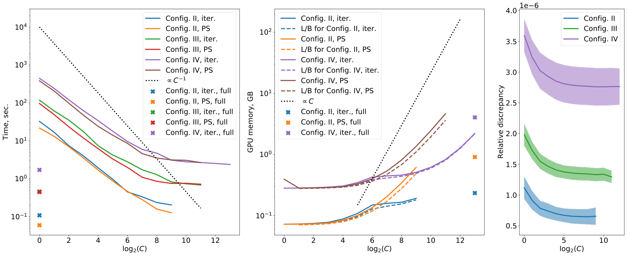
We run Algorithm 1 for configurations II-IV and different powers of 2 as $C$. We use input strings sampled randomly from $\Sigma^{L}$. In order to characterize the time-memory tradeoff, we measure wall-clock time and peak GPU memory for a single gradient evaluation. We use the torch.cuda.max_memory_allocated function to report peak GPU memory.

As discussed in Section 2.1, there are two methods to compute (3-4): the first (iterative) method doesn’t compute and store tensors (4) explicitly, resulting in smaller memory consumption at a cost of less parallelization, while the second one computes tensors (4) using the parallel prefix sum algorithm, therefore operating faster, but using more memory. The same methods can be applied for the memory-efficient algorithm when computing (17-18) updates. We implement and benchmark both methods as part of the algorithm. For the explicit prefix-sum method, we find that the torch.cumsum function works faster and consumes less memory than our custom implementation of the parallel prefix sum algorithm. We attribute this to hardware-optimized low-level implementation of the native function, and use this function in experiments. As for the iterative algorithm, we implement its “block” version, when, instead of iterating $l$ one-by-one, we iterate through blocks of small size (see details in Appendix B). This way, the algorithm has a smaller constant in $O(L)$ time complexity and bigger constant in a “small” $O(dM)$ term of the memory complexity (assuming that $d,M\ll L$).

For a fixed value of $C$, in addition to benchmarking memory of Algorithm 1, we also report memory of the naive gradient computation run on a string of length $C$, sampled uniformly from $\Sigma^{C}$. This is to confirm that memory consumption of Algorithm 1 is just slightly above the full computation on the input of length $C$.

Results are reported in Figure 2 (left, middle). We observe significant improvements in memory consumption compared to the full computation, as $C$ decreases. As $C$ converges to $2^{0}=1$, the remaining memory consumption can be attributed to storage of the model’s parameters $\theta$. Time follows two regimes: declining fast as $C$ grows (meaning that prefix sums are parallelized) and declining slower for big values of $C$ (meaning that the practical limit of parallelization is reached). Memory scales slower than $O(C)$, as $C$ increases. We attribute this effect to details of PyTorch internal implementation. Interestingly, we find that iterative version of (3-4) computation works only slightly slower than prefix-sum version, while consuming much less memory. Finally, Algorithm 1 consumes slightly more memory in practice than the full method run on the input of length $C$.

Since the iterative version of (3-4) computation results in a good balance between time and memory of Algorithm 1, we use it in our subsequent experiments. To quantify finite-precision effects, we plot relative discrepancy $\|\nabla_{\theta}^{(C)}\mathcal{L}-\nabla_{\theta}^{(full)}\mathcal{L}\|_{2}/\|\nabla_{\theta}^{(full)}\mathcal{L}\|_{2}$ between the gradient $\nabla_{\theta}^{(C)}$ produced by Algorithm 1, and the gradient $\nabla_{\theta}^{(full)}\mathcal{L}$ produced by full-input computation. Figure 2 illustrates results for randomly initialized models. We observe a very small discrepancy (of order $10^{-6}$–$10^{-5}$), confirming the correctness of Algorithm 1. The discrepancy is slightly increasing as $C$ decreases, which can be attributed to effects of finite-precision arithmetic.

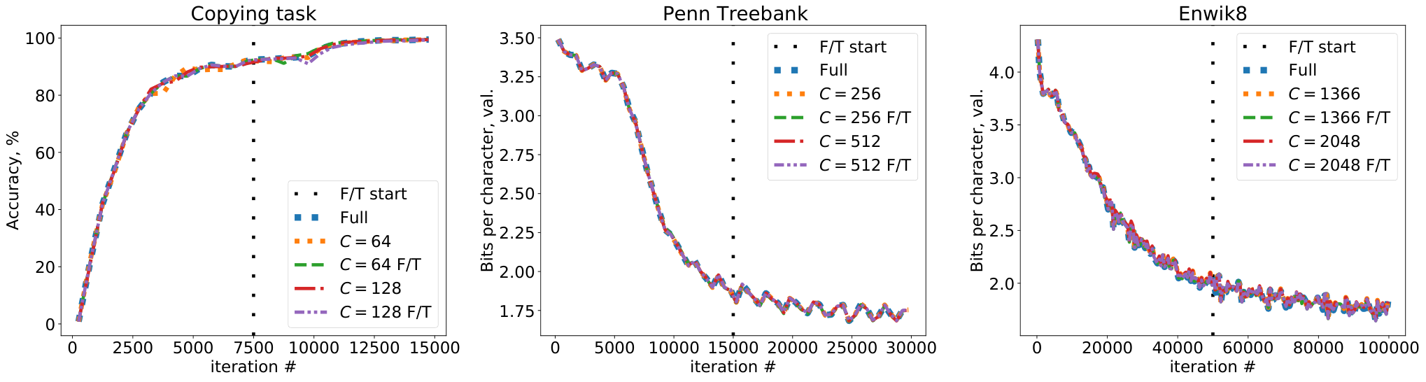
To confirm backward compatibility of Algorithm 1 during training, we consider three language modelling setups: Copying task, symbol-level Penn Treebank and Enwik8.

For the Copying task, we follow the setup from (Kitaev et al. 2020; Katharopoulos et al. 2020), sampling inputs as $0\omega 0\omega$, where $\omega$ is drawn uniformly from $(\Sigma\setminus\{0\})^{L/2-1}$. In this setup, we only aggregate cross-entropy loss from the second half of the input, so the task is to reproduce the first half. We include the Copying task as an example setup where long-range information propagation is crucial, and the heuristic of “chunking” the input into smaller segments would fail to solve the task.

We use model configurations I, II, III for the Copying task, Penn Treebank and Enwik8 respectively, resulting in sequence lengths $L=512,1024,4096$ respectively. For each setup, we compare training with full gradient computation, and training equipped with memory-efficient gradient computation via Algorithm 1 using various values of $C$. In addition, we consider a “fine-tuning” regime, when the first half of iterations is run using the full algorithm, and the second half is run using Algorithm 1. Figure 3 demonstrates results: all methods result in the same, indistinguishable performance. This confirms that memory-efficient gradient computation can be used both for training from scratch, and for fine-tuning, e.g. on a low-memory device. Table 2 quantifies the memory savings and time tradeoff in all setups. Additional experimental details and results (bigger version of Figure 3, bits-per-character for the Copying task and train set performance for Penn treebank and Enwik8) can be found in Appendix C.

References

- Abadi et al. (2015) Abadi, M., Agarwal, A., Barham, P., Brevdo, E., Chen, Z., Citro, C., Corrado, G. S., Davis, A., Dean, J., Devin, M., Ghemawat, S., Goodfellow, I., Harp, A., Irving, G., Isard, M., Jia, Y., Jozefowicz, R., Kaiser, L., Kudlur, M., Levenberg, J., Mané, D., Monga, R., Moore, S., Murray, D., Olah, C., Schuster, M., Shlens, J., Steiner, B., Sutskever, I., Talwar, K., Tucker, P., Vanhoucke, V., Vasudevan, V., Viégas, F., Vinyals, O., Warden, P., Wattenberg, M., Wicke, M., Yu, Y., and Zheng, X. TensorFlow: Large-scale machine learning on heterogeneous systems, 2015. URL https://www.tensorflow.org/. Software available from tensorflow.org.
- Ba et al. (2016) Ba, J. L., Kiros, J. R., and Hinton, G. E. Layer normalization. arXiv preprint arXiv:1607.06450, 2016.
- Brown et al. (2020) Brown, T. B., Mann, B., Ryder, N., Subbiah, M., Kaplan, J., Dhariwal, P., Neelakantan, A., Shyam, P., Sastry, G., Askell, A., Agarwal, S., Herbert-Voss, A., Krueger, G., Henighan, T., Child, R., Ramesh, A., Ziegler, D. M., Wu, J., Winter, C., Hesse, C., Chen, M., Sigler, E., Litwin, M., Gray, S., Chess, B., Clark, J., Berner, C., McCandlish, S., Radford, A., Sutskever, I., and Amodei, D. Language models are few-shot learners, 2020.
- Chen et al. (2018) Chen, R. T. Q., Rubanova, Y., Bettencourt, J., and Duvenaud, D. K. Neural ordinary differential equations. In Bengio, S., Wallach, H., Larochelle, H., Grauman, K., Cesa-Bianchi, N., and Garnett, R. (eds.), Advances in Neural Information Processing Systems, volume 31, pp. 6571–6583. Curran Associates, Inc., 2018. URL https://proceedings.neurips.cc/paper/2018/file/69386f6bb1dfed68692a24c8686939b9-Paper.pdf.
- Chen et al. (2016) Chen, T., Xu, B., Zhang, C., and Guestrin, C. Training deep nets with sublinear memory cost. CoRR, abs/1604.06174, 2016. URL http://arxiv.org/abs/1604.06174.
- Child et al. (2019) Child, R., Gray, S., Radford, A., and Sutskever, I. Generating long sequences with sparse transformers. CoRR, abs/1904.10509, 2019. URL http://arxiv.org/abs/1904.10509.
- Cho et al. (2014) Cho, K., van Merriënboer, B., Gulcehre, C., Bahdanau, D., Bougares, F., Schwenk, H., and Bengio, Y. Learning phrase representations using RNN encoder–decoder for statistical machine translation. In Proceedings of the 2014 Conference on Empirical Methods in Natural Language Processing (EMNLP), pp. 1724–1734, Doha, Qatar, October 2014. Association for Computational Linguistics. doi: 10.3115/v1/D14-1179. URL https://www.aclweb.org/anthology/D14-1179.
- Choromanski et al. (2020) Choromanski, K., Likhosherstov, V., Dohan, D., Song, X., Gane, A., Sarlos, T., Hawkins, P., Davis, J., Mohiuddin, A., Kaiser, L., Belanger, D., Colwell, L., and Weller, A. Rethinking attention with Performers. CoRR, arXiv:2009.14794, 2020. URL https://arxiv.org/abs/2009.14794.
- Dai et al. (2019) Dai, Z., Yang, Z., Yang, Y., Cohen, W. W., Carbonell, J., Le, Q. V., and Salakhutdinov, R. Transformer-XL: Language modeling with longer-term dependency, 2019. URL https://openreview.net/forum?id=HJePno0cYm.
- Griewank (1992) Griewank, A. Achieving logarithmic growth of temporal and spatial complexity in reverse automatic differentiation. Optimization Methods and Software, 1(1):35–54, 1992. doi: 10.1080/10556789208805505. URL https://doi.org/10.1080/10556789208805505.
- Griewank & Walther (2008) Griewank, A. and Walther, A. Evaluating Derivatives: Principles and Techniques of Algorithmic Differentiation, Second Edition. Other Titles in Applied Mathematics. Society for Industrial and Applied Mathematics (SIAM, 3600 Market Street, Floor 6, Philadelphia, PA 19104), 2008. ISBN 9780898717761. URL https://books.google.co.uk/books?id=xoiiLaRxcbEC.
- Hendrycks & Gimpel (2016) Hendrycks, D. and Gimpel, K. Bridging nonlinearities and stochastic regularizers with gaussian error linear units. CoRR, abs/1606.08415, 2016. URL http://arxiv.org/abs/1606.08415.
- Hochreiter & Schmidhuber (1997) Hochreiter, S. and Schmidhuber, J. Long short-term memory. Neural Comput., 9(8):1735–1780, November 1997. ISSN 0899-7667. doi: 10.1162/neco.1997.9.8.1735. URL http://dx.doi.org/10.1162/neco.1997.9.8.1735.
- Katharopoulos et al. (2020) Katharopoulos, A., Vyas, A., Pappas, N., and Fleuret, F. Transformers are RNNs: Fast autoregressive transformers with linear attention. arXiv preprint arXiv:2006.16236, 2020.
- Kingma & Ba (2015) Kingma, D. P. and Ba, J. Adam: A method for stochastic optimization. In Bengio, Y. and LeCun, Y. (eds.), 3rd International Conference on Learning Representations, ICLR 2015, San Diego, CA, USA, May 7-9, 2015, Conference Track Proceedings, 2015. URL http://arxiv.org/abs/1412.6980.
- Kitaev et al. (2020) Kitaev, N., Kaiser, L., and Levskaya, A. Reformer: The efficient transformer. In 8th International Conference on Learning Representations, ICLR 2020, Addis Ababa, Ethiopia, April 26-30, 2020. OpenReview.net, 2020. URL https://openreview.net/forum?id=rkgNKkHtvB.
- Ladner & Fischer (1980) Ladner, R. E. and Fischer, M. J. Parallel prefix computation. J. ACM, 27(4):831–838, October 1980. ISSN 0004-5411. doi: 10.1145/322217.322232. URL https://doi.org/10.1145/322217.322232.
- Lan et al. (2020) Lan, Z., Chen, M., Goodman, S., Gimpel, K., Sharma, P., and Soricut, R. ALBERT: A lite BERT for self-supervised learning of language representations. In International Conference on Learning Representations, 2020. URL https://openreview.net/forum?id=H1eA7AEtvS.
- Li et al. (2020) Li, R., Duan, C., and Zheng, S. Linear attention mechanism: An efficient attention for semantic segmentation. arXiv preprint arXiv:2007.14902, 2020.
- Mahoney (2009) Mahoney, M. Large text compression benchmark, 2009.
- Marcus et al. (1993) Marcus, M. P., Santorini, B., and Marcinkiewicz, M. A. Building a large annotated corpus of English: The Penn Treebank. Computational Linguistics, 19(2):313–330, 1993. URL https://www.aclweb.org/anthology/J93-2004.
- Ott et al. (2018) Ott, M., Edunov, S., Grangier, D., and Auli, M. Scaling neural machine translation. In Proceedings of the Third Conference on Machine Translation: Research Papers, pp. 1–9, Brussels, Belgium, October 2018. Association for Computational Linguistics. doi: 10.18653/v1/W18-6301. URL https://www.aclweb.org/anthology/W18-6301.
- Ott et al. (2019) Ott, M., Edunov, S., Baevski, A., Fan, A., Gross, S., Ng, N., Grangier, D., and Auli, M. fairseq: A fast, extensible toolkit for sequence modeling, 2019.
- Parisotto et al. (2019) Parisotto, E., Song, H. F., Rae, J. W., Pascanu, R., Gulcehre, C., Jayakumar, S. M., Jaderberg, M., Kaufman, R. L., Clark, A., Noury, S., et al. Stabilizing transformers for reinforcement learning. arXiv preprint arXiv:1910.06764, 2019.
- Parmar et al. (2018) Parmar, N., Vaswani, A., Uszkoreit, J., Kaiser, L., Shazeer, N., and Ku, A. Image transformer. CoRR, abs/1802.05751, 2018. URL http://arxiv.org/abs/1802.05751.
- Paszke et al. (2017) Paszke, A., Gross, S., Chintala, S., Chanan, G., Yang, E., DeVito, Z., Lin, Z., Desmaison, A., Antiga, L., and Lerer, A. Automatic differentiation in pytorch. 2017.
- Radford et al. (2019) Radford, A., Wu, J., Child, R., Luan, D., Amodei, D., and Sutskever, I. Language models are unsupervised multitask learners. OpenAI Blog, 1(8):9, 2019.
- Roy et al. (2020) Roy, A., Saffar, M., Vaswani, A., and Grangier, D. Efficient content-based sparse attention with routing transformers. arXiv, 2003.05997, 2020.
- Sanh et al. (2020) Sanh, V., Debut, L., Chaumond, J., and Wolf, T. DistilBERT, a distilled version of BERT: smaller, faster, cheaper and lighter. arXiv, 1910.01108, 2020.
- Shen et al. (2018) Shen, Z., Zhang, M., Yi, S., Yan, J., and Zhao, H. Factorized attention: Self-attention with linear complexities. CoRR, abs/1812.01243, 2018. URL http://arxiv.org/abs/1812.01243.
- Srivastava et al. (2014) Srivastava, N., Hinton, G., Krizhevsky, A., Sutskever, I., and Salakhutdinov, R. Dropout: A simple way to prevent neural networks from overfitting. Journal of Machine Learning Research, 15(56):1929–1958, 2014. URL http://jmlr.org/papers/v15/srivastava14a.html.
- Tay et al. (2020a) Tay, Y., Dehghani, M., Abnar, S., Shen, Y., Bahri, D., Pham, P., Rao, J., Yang, L., Ruder, S., and Metzler, D. Long range arena: A benchmark for efficient transformers. arXiv, 2011.04006, 2020a.
- Tay et al. (2020b) Tay, Y., Dehghani, M., Bahri, D., and Metzler, D. Efficient transformers: A survey. arXiv, 9.20006732, 2020b.
- Vaswani et al. (2017) Vaswani, A., Shazeer, N., Parmar, N., Uszkoreit, J., Jones, L., Gomez, A. N., Kaiser, L. u., and Polosukhin, I. Attention is all you need. In Guyon, I., Luxburg, U. V., Bengio, S., Wallach, H., Fergus, R., Vishwanathan, S., and Garnett, R. (eds.), Advances in Neural Information Processing Systems 30, pp. 5998–6008. Curran Associates, Inc., 2017. URL http://papers.nips.cc/paper/7181-attention-is-all-you-need.pdf.
- Vishkin (2010) Vishkin, U. Thinking in parallel: Some basic data-parallel algorithms and techniques. 2010.
- Wu* et al. (2020) Wu*, Z., Liu*, Z., Lin, J., Lin, Y., and Han, S. Lite transformer with long-short range attention. In International Conference on Learning Representations, 2020. URL https://openreview.net/forum?id=ByeMPlHKPH.
- Xiong et al. (2020) Xiong, R., Yang, Y., He, D., Zheng, K., Zheng, S., Xing, C., Zhang, H., Lan, Y., Wang, L., and Liu, T.-Y. On layer normalization in the transformer architecture, 2020.
- You et al. (2019) You, Y., Li, J., Hseu, J., Song, X., Demmel, J., and Hsieh, C. Reducing BERT pre-training time from 3 days to 76 minutes. CoRR, abs/1904.00962, 2019. URL http://arxiv.org/abs/1904.00962.
Appendix A Derivation of gradient expressions
doesn’t affect terms , so corresponding gradients are zero:
Similarly, does not affect , so
In particular,
For all , and affect only through , so according to the chain rule
where denotes Jacobian matrices. Further, for all :
where . denotes a stop-gradient operator, i.e. gradients are not propagated inside brackets and the argument is considered as constant.
Appendix B Efficient “Block” Computation of (3-4)
Denote , , , . Katharopoulos et al. 2020 propose the following algorithm for computation of (3-4). Initialize buffers , iterate over and compute
This way, 3d tensor is not stored in memory explicitly, resulting in time and memory complexity. In order to have the same memory consumption during back-propagation, Katharopoulos et al. 2020 propose the following routine. Keep buffers as the result of forward pass, and initialize gradient buffers . Assuming that are computed using automatic differentiation, iterate in a backward direction and compute
In practice, the described algorithm works slow when implemented in pure PyTorch, because is iterated one-by-one: Katharopoulos et al. 2020 use low-level CUDA extensions to make the algorithm practical. Instead, we propose a “block” version, when we iterate through blocks of of a small size (we use ). In each block use explicit prefix sums on inputs of length to find , using the maintained front . The formal algorithm is as follows. Initialize buffers . For simplicity assuming that divides (extension for an opposite case is straightforward), iterate over and compute