Supplementary Materials for: Witnessing quantum correlations in a nuclear ensemble via an electron spin qubit
I Experimental techniques
A Quantum dot devices
Data was taken on two QD devices, made from the same wafer. QD device 1 was used in previous studies Bodey2019; Stockill2016; Ethier-Majcher2017; Huthmacher2018, and is the device on which the data was taken throughout the main text and this supplement, unless otherwise stated. QD device 2 was used in previous studies Gangloff2019, and is the device used for some of the data sets presented in this supplement.
Self-assembled InGaAs QDs are grown by molecular beam epitaxy and integrated inside a Schottky diode structure to allow charge control Urbaszek2013. This comprises a 35nm tunnel barrier between the n-doped layer and the QDs, and a blocking barrier above the QD layer to prevent charge leakage. The Schottky diode structure is electrically contacted through ohmic AuGeNi contacts to the n-doped layer and a semitransparent Ti gate (6 nm) is evaporated onto the surface of the sample. A distributed Bragg reflector below the QDs maximises photon outcoupling efficiency. The photon collection is further enhanced with a superhemispherical cubic zirconia solid immersion lens on the top Schottky contact of the device. We estimate a photon-outcoupling efficiency of 10% at the first lens for QDs with an emission wavelength around 970 nm.
B Experimental schematic

A schematic of the experiment is shown in Fig. S1. A helium bath cryostat houses the QD device at 4K. A magnetic field T is applied transverse to the QD growth axis (Voigt geometry). Two laser beams are combined and sent to the QD: a Raman laser system, which is microwave-modulated, and a resonant readout/repump laser (MogLabs diode laser). A cross-polarisation confocal microscope filters resonant laser background, and a grating removes non-resonant background. The filtered signal is sent to a superconducting nanowire single photon detector (SNSPD, Quantum Opus One).
C Laser system
The Raman laser system is based on a Toptica BoosTA tapered amplifier seeded by a Toptica DL Pro diode laser. This is far-detuned from the optically excited states by GHz. This travels through a fibre-based EOSPACE electro-optic modulator (EOM) which is driven with a microwave waveform. The microwave waveform is generated by mixing a Rohde&Schwarz LO microwave source (operated at GHz) with the signal from a Tektronix arbitrary waveform generator (AWG70001A, 25 GS/s) (operated around MHz). An Analog Devices wideband microwave IQ-mixer frequency-doubles the Rohde&Schwarz signal, and downshifts it using the AWG signal.
The first-order sidebands of the optical field after the EOM are two coherent laser fields, separated in frequency by twice the microwave drive frequency . These Raman beams pass through a quarter-wave plate, arriving at the QD with a circular polarisation. They address the electron spin states with a two-photon detuning (i.e. Raman frequency) of .
D Polarisation dragging sequence
We control the mean-field nuclear polarisation by tuning the frequency of the Rohde&Schwarz LO source whilst running the experimental sequence, which consists mostly of cooling. Tuning the LO in turn tunes , altering the stable lockpoint of the feedback function (see Fig. 1 of the main text). We begin a sequence at zero polarisation, where the Raman sideband splitting corresponds to the electron Zeeman energy. From there, we increase the sideband splitting (two-photon detuning/Raman frequency ) by increasing the Rohde&Schwarz frequency. The linear range of the feedback (Fig. 1e, main text) is set by the nuclear Zeeman energy (). During the preparation of a polarised state, the frequency is increased in steps of 1 MHz, to stay well within this linear regime of feedback. Also, the electron spin resonance (ESR) is increased at a rate of . In this way, we are able to drag the electron spin resonance over a GHz range for QD device 1, and over a GHz range for QD device 2 (as in Fig. S2). We compensate the unwanted shift in transition frequency to the optical excited state, due to the Overhauser shift of the ground and excited states, by applying a compensating linear ramp to the QD device gate voltage. This tunes the trion transition frequency via the DC Stark shift. Left unchecked, the generated Overhauser shift would cause our repump laser to lose resonance. A typical resonance fluorescence signal for this dragging process is shown in Fig. S2, where the falling edges indicate a loss of feedback stability on the mean-field shift, as described in the main text. When taking magnon spectra (e.g. Fig. 1 of the main text), the polarisation sequence is stopped before this loss of stability and of resonance fluorescence.
E Experimental spectroscopy sequence
In Figs. 1f and 2a of the manuscript, we use a time-averaged measurement, with the following elementary sequence:
- 1.
We cool the nuclei optically for . This step uses an optical Raman scheme detailed in Gangloff2019. We optimise the cooling parameters by operating under conditions which maximise the electron - an inhomogeneous dephasing time, inversely proportional to the magnitude of nuclear polarisation fluctuations. The relevant settings during the cooling sequence are: a Raman Rabi frequency MHz and a repump Rabi frequency of for an excited state linewidth MHz. This gives us an optimal of , over an order of magnitude longer than without cooling.
- 2.
We probe the nuclei for . In this step, we first initialise the electron spin. We then measure the electron spin-state population after a single ESR probe pulse of duration , of electron Rabi frequency MHz and at a given detuning (i.e. relative to the preparation). The electron spin-initialisation and read-out pulses are both 100ns: a pulse from the resonant readout/repump laser excites population from to one of the trion excited states; from there, it decays radiatively into the ground state manifold (Fig. S1); the pulse length is much longer than the excited state lifetime. The collected fluorescence is proportional to the population of ; and at the end of this readout/repump pulse, the electron is into . The remainder in this step is “dead-time”, where no control pulses act on the electron.
This elementary sequence (prep+single probe of the spectrum at a fixed ) is repeated 2,400,000 times per data point (60s of integration). Then we step by 4MHz, and perform another time-averaged measurement at this new detuning.
Figure 2b presents a measurement which also alternates a cooling and a probe step, but where we instead scan the length of the ESR probe pulse at a fixed . During this measurement, we pair two pulses of increasing and decreasing lengths such that total Raman power is conserved, allowing us to stabilise the time-averaged laser power to within 1%.
We keep the time ratio of cooling-to-spectroscopy around 20-to-5, meaning that we spend 80% of the time cooling the nuclear ensemble. This ensures that the steady-state of the nuclear ensemble is primarily determined by the cooling sequence Jackson2020.
F Data processing and normalisation
F.1 Background subtraction
Our raw measurements of the magnon spectrum include a constant background count rate, as determined by the readout signal we obtain at large Raman detuning . This is due to optically induced electron spin relaxation, via a mechanism external to the QD Bodey2019. We subtract this constant background, which is equal to the count rate at large Raman detuning , from our data. When integrated over a typical spectrum, the background count rate constitutes of the uncorrected signal.
F.2 Polarisation-dependent count rate
We observe a systematic decrease in count rate as the nuclear ensemble is polarised so as to increase the mean-field shift on the ESR. This is because the collected readout fluorescence passes through a narrowband ( GHz) optical grating in order to remove the laser background from the far-detuned Raman beams. When we polarise, Raman photon emission will change in frequency due to the change in ESR splitting. The collection efficiency of Raman photons therefore decreases as nuclear polarisation increases from zero. In order to correct for this effect, we normalise data taken at each polarisation by its average count rate.
F.3 From count rate to electron-spin population
Throughout the main text, read-out fluorescence counts have been converted to electron population. In Figs. 1, 2(a), and 3 we use the fit to the time evolution of the magnon spectrum (later presented in Fig. S10) to fix the count rate which corresponds to 50% population. In Fig. 2(b), we assume that the system, when on resonance with the ESR, will reach a steady-state of 50% population at long drive time.
II Model
A System Hamiltonian
The effective Hamiltonian of the system for a single spin species is given by Gangloff2019:
| (1) |
The first two terms model the ESR drive, in the frame rotating with the frequency of the drive. The third term introduces a nuclear Zeeman interaction. The fourth term stands for the hyperfine interaction between the central electron and the nuclei, in the limit of a high external magnetic field. The hyperfine constant per nucleus is taken constant for a given species (a box approximation: ). The sums run over the nuclei of that species.
Moreover:
| (2) |
are the terms originating from the strain-induced quadrupolar interaction, that offset the quantisation axis, thus introducing a correction to the hyperfine interaction.
The term , derived perturbatively via the Schrieffer-Wolff transformation, enables the coherent electron-nuclear exchange. In particular, the magnon injection is effectuated by the action of the spin-wave operators:
| (3) |
Where we distinguished collective and single-spin operators and , respectively, for processes changing the nuclear polarisation by one () or two () units.
Within a single-spin manifold transition between and is not allowed due to the form of .
B Relating Exchange frequencies to spin-state populations and polarisation
Action of the operator on the initial (pure) state will bring it to
| (4) |
At times when dynamics are restricted to the manifold, the electron-nuclear exchange frequency is proportional to the matrix element of the operator
| (5) |
where is the Rabi frequency of the ESR drive. Assuming that the system is initialised in a pure product state:
| (6) |
the exchange frequency is found as
| (7) |
Across a single spin- species, the above sum can be reduced to a sum over single spin states weighed by their fractional populations , , …, , such that
| (8) |
where constants were defined in Eq. 3, and are numerical pre-factors resulting from the form of the single-spin magnon laddering operators, given explicitly by
| (9) |
It should be noted that away from zero polarisation, the enhancement factors differ among the sideband transitions, and directly reflect the populations of single spin states.
One can relate the exchange frequencies for all four sideband processes to the polarisation of partaking spin owing to the identity:
| (10) |
which translates to:
| (11) |
B.1 Exact treatment of
For the particular case of , Eq. 8 gives:
| (12) |
where we substituted back in the exact expressions for from Eq. 3. Since , the assumption of an initial product state leads to the emergence of two constants of motion:
| (13) |
This motivates the definition of a self-referenced dimensionless parameter - the magnon asymmetry - as in Eq. 3 of the main text.
Magnon asymmetries for both first and second sideband processes are linked to the single spin state populations via:
| (14) |
which is used to arrive at the expressions in Eqs. 4 and 5 of the main text.
The constants of motion (Eq. 13) are crucial to go beyond Eq. 11 and establish a self-referenced measure of the polarisation of a spin , for any distribution of population. For a spin , the quantity is no longer constant in general, and we must assume a type of population distribution in order to link the magnon sideband asymmetry to polarisation.
B.2 Treatment of with thermal-state approximation
Equation 5 of the main text, which equates the measured quantity to the single-species polarisation , is a definition that holds true only for . For we still measure the same quantity (), but as we will show below, in this case it slightly underestimates the polarisation.
Our definition imposes to match for a thermal state of any spin . We use this to generalise to higher-spin species. For a thermal state we can straightforwardly calculate (which is our definition of ) and (which is the experimentally measured parameter). Plotting the former against the latter yields Fig. S3, and gives us the high-spin correction to Eq. 5 of the main text. Figure S3 shows that is an underestimate of the polarisation .
We have used this function to reconstruct the polarisation of indium () shown in Fig. 4a of the main text, from measurements of its magnon mode asymmetry. The feedback-induced deviations of the spin-state populations from those of a thermal state, already small for spin- species (see Fig. 3b, main text), should be even smaller for a spin- species such as indium. This scaling operation (up to a factor 2) thus presents a more realistic estimate of the indium contribution to the Overhauser field. Treating indium as a spin- species instead (no scaling), the asymmetry-commensurate Overhauser field would exceed the classical bound by 1.9(1).
B.3 Mixed state
The above considerations are generalised easily to arbitrary states (including mixed states), through:
| (15) |
where stands for a density operator, representative of the nuclear state of the system. In the case of a mixture of product states considered in Eq. 6, the statements involve the expectation values of polarisation, and manifold imbalances. The consequence of non-vanishing steady-state coherences is discussed in section VI.
III Complementary Measurements
A Homogeneous dephasing
We measure the electron spin dephasing time using the Hahn echo sequence, which consists of two pulses separated by an echo time, and a refocusing pulse placed at half the echo time. The pulse filters noise which is static over the duration of the pulse sequence, and tuning the phase of the final pulse allows the remaining coherence of the electron spin to be measured. Figure S4 depicts the dependence of the Hahn echo visibility on echo time yielding a Hahn-Echo time of s.
B Inhomogeneous dephasing
We measure using Ramsey interferometry Stockill2016. In the time domain, we observe a Gaussian decay profile of the electron spin coherence which we fit with . Figure S5 presents the values measured with increasing polarisation. Our data is polarisation-independent within error bars and equal to (solid line in Fig. S4).
The inhomogeneous dephasing time, , appears throughout the experiment as a limit on spectral resolution: the effect of the inhomogeneous dephasing on the magnon spectrum is equivalent to that of a Gaussian convolution filter, with width:
| (16) |
is set by the performance of the nuclear preparation - see section V for a complete discussion of mechanisms that influence it.
C Hyperspectral map of magnon modes
We have measured the magnon spectrum as a function of the Raman drive time from to s, at a near-zero mean-field shift. The resulting two-dimensional map, shown in the left-most panel of Fig. S10, shows the electron-spin population as a function of ESR detuning and Raman drive time. This data is used to constrain the dephasing of magnon modes in the magnon spectrum modelling, as analysed in section C.
D Nuclear spin decay
Using QD device 2 at a field T, we measure the relaxation of the mean-field shift following its preparation at a GHz electron-spin splitting (the electron-spin splitting at zero nuclear polarisation is GHz). The cooling beams (Raman and resonant) are turned off and a waiting time from to s follows. The resonant beam is then turned on again as the gate is swept across all four trion state resonances, allowing us to infer the electron spin splitting spectrally. The result is shown in Fig. S6, where the data clearly exhibits two relaxation timescales. Using a biexponential fit, we find that the initial fast decay of of the mean-field polarisation occurs over a characteristic time ms, while the slower decay occurs over a characteristic time s.
This fitted timescale is relevant to our modelling of the cooled nuclear spin populations in section A.2, where it sets a constraint on the nuclear spin diffusion rate that limits the cooling.
The fitted timescale exceeds by a factor of our electron-spin relaxation time of a few tens of s; this process is dominated by coupling to the back-contact (tunnel barrier of 35 nm in our devices, see section A). For identical magnetic field of T, this is in close quantitative agreement with recent reports on the ratio of electron and nuclear spin relaxation times for tunnel barriers below 42 nm Gillard2021. The parameter is not used further in our analysis.

We also measure the characteristic relaxation time of the mean-field fluctuations, which are reduced from thermal equilibrium by our optical cooling, as a function of the mean field. Following the preparation of a variable electron spin splitting using our polarisation sequence, we turn the cooling beams off, introduce a wait time up to 200 ms, and measure the electronic using a Ramsey interferometry sequence. We find that the variance of the mean-field, , relaxes exponentially with a characteristic correlation time Ethier-Majcher2017. This correlation time is shown as a function of the prepared electron spin splitting in Fig. S7. We find that the correlation time for mean-field values leading to electron-spin splittings of GHz is the same as the ms measured as a fast decay of the mean field itself in Fig. S6. We also see that, with the exception of extremal points close to regions of instability, the correlation grows quadratically with the electron spin splitting (solid curve in Fig. S7). Taken together, these observations point to a fast nuclear relaxation mechanism for the mean-field statistics (both mean and variance) governed by electronic degrees of freedom; a plausible candidate is the three-body RKKY-type interaction that arises in the second-order of the hyperfine interaction Wust2016.

E ESR offset,
The hyperspectral magnon map shown in Fig. 1f of the main text, as a function of Raman detuning and mean-field shift , exhibits a MHz-scale offset that scales linearly with the GHz-scale mean-field shift – owing to a nuclear polarisation-induced shift in the nuclear feedback curve (main text Fig. 1e). In more detail, we extract from a fit to the unfiltered spectra of Fig. 1f, as an overall offset common to all sideband and ESR features. We show as a function of mean-field shift in Fig. S8.
The ESR detuning is then defined as a corrected Raman detuning: .
IV Supplementary notes on data analysis
A Wiener deconvolution
Fitting the magnon spectrum with a model that accounts for an electron process – i.e. a convolution with a Gaussian profile of width given by Eq. 16 – is computationally intensive. Since is known through an independent measurement (section B), its effect can be factored out by deconvolving prior to fitting. This significantly reduces the computational cost of the fitting procedure. In the face of noise inherent to any real measurement, deconvolution has to be done with great care. Here we outline how this can be optimally achieved.
The Fourier transform of the data - - is expected to be of the form:
| (17) |
where and are the Fourier transforms of the Gaussian with width and of the signal that we wish to extract, respectively.
Multiplying directly by the inverse Gaussian filter:
| (18) |
where is taken from Eq. 16, would amplify the high-frequency part of noise , and would distort the filtered signal . Instead, we use the Wiener filter wiener2013extrapolation:
| (19) |
where the constant should be set close to the ratio of noise-to-signal spectral densities (). Without a priori knowledge of the spectral noise density, we find by optimizing the filtering performance.
The main contributions to come from drifts that we take as uncorrelated with signal. This guarantees that for the optimal , the mean-square error of the extracted signal and the true signal, namely:
| (20) |
is minimised. For each value of taken from a broad range ( - ), we fit the deconvolved spectra with our model (section B) and evaluate the sum of the squared residuals. This sum (orange curve in Fig. S9) is minimised for , which we conclude to be the optimal filtering parameter.

We further assess the goodness of the fit against the raw data. We convolve the fitted model and evaluate the sum of the squared residuals (purple curve in Fig. S9). This sum reaches a minimum below , and increases for below where excessive amplification of high frequencies of the noise occurs. The Wiener filter at operates close to this minimum, and has the benefit of simultaneously minimising the from Eq. 20.
B Model function used to fit the data
When modelling the ESR drive, or any of the sideband processes, we approximate the time evolution of their lineshapes as that of independent two-level systems (TLSs), each governed by the following optical Bloch equations:
| (21) |
Here the dissipative dynamics are modelled by Lindblad operators . In the Bloch vector representation, i.e. , the optical Bloch equations are equivalent to:
| (22) |
Where . The time evolution of the Bloch vector is then found as:
| (23) |
where the steady state Bloch vector components are:
| (24) |
The magnon spectrum and its time dependence (in the absence of optical pumping) are broadened and damped by three types of processes:
- •
Inhomogeneous dephasing - a process,
- •
Homogeneous pure dephasing - a process,
- •
Slow, optically induced process, modelled by .
The optically induced process is subtracted from the data, as described in section F.1. The effects are factored out through a Wiener deconvolution, as described in section A. Since, under the above conditions, the TLS saturates to , the lineshapes undergo expansion from their short-time limit to infinitely wide, allowing the rate of homogeneous pure dephasing to be constrained by a fit to the time dependence of the spectrum.
C Setting dephasing times from the magnon spectrum time-dependence
Following the application of a Wiener deconvolution to the data (section A), nine independent TLS models (section B) are fitted to the time dependence of the magnon spectrum, as shown in Fig. S10. The lineshape at MHz corresponds to the central ESR. The lineshapes at , for MHz correspond to the first and second sideband transitions of the arsenic species, and those at , for MHz are the same transitions of the indium species. The ESR Rabi frequency is fitted as , whereas the exchange frequencies for the sideband transitions are all of the order .
From the fit shown in Fig. S10, we obtain the pure dephasing times for the ESR, arsenic magnons, and indium magnons:
- •
Electron homogeneous dephasing time, fitted as . We note that this (section A) as the continuous Rabi drive dynamically decouples the electron spin beyond the simple Hahn-Echo time.
- •
Pure dephasing time for electron-arsenic interaction,
- •
Pure dephasing time for electron-indium interaction,
We do not resolve features arising from interactions with gallium nuclei, and therefore do not include them in our fitting. This is consistent with our previous reports of magnons in these systems Gangloff2019; Jackson2020, and is likely to stem from gallium’s weaker quadrupolar coupling Stockill2016. Taking typical literature values for its quadrupolar constant and quadrupolar angle Bulutay2012, alongside its Zeeman energy, we expect gallium’s magnon modes to be a factor of 15 (4) weaker than those for arsenic, for processes changing by 1 (2) unit(s) Jackson2020. Given that arsenic and indium interactions are already weak compared to their dephasing rates, we can safely neglect all modes relating to gallium.
D Fitting the species-resolved spectra (data presented in the main text)
With the dephasing parameters fixed from the fit in the previous section (C), we now focus on individual spectra taken at a s drive time, for a range of mean-field shifts: to GHz in steps of GHz. We let the fit identify the relative offset of the centre of the ESR peak (, see also section E), and leave the Zeeman frequencies for indium and arsenic as free parameters. On top of these three parameters, the exchange frequencies for each of the sideband transitions (, , , for ) are fitted from the TLS lineshape at drive time (see section B).
A summary of fitted exchange frequencies is shown in Fig. S11. Figure 3a from the main text illustrates the sum of the nine lineshapes that constitutes a fit to the deconvolved spectrum.
The fitted Zeeman frequencies and central peak offset are plotted in Fig. S12, together with error bars. Orange data points are associated to indium, purple to arsenic. Dashed lines stand for the Zeeman frequencies of indium and arsenic under an external magnetic field of T, converted from their nuclear -factors found in the literature Stockill2016: MHz, MHz.
The piecewise constant structure in the fitted central peak offset is an artefact of the fit’s initial guess on the offset being identified with the position of the maximum point within the central peak. Since changing by a small amount, while holding other parameters constant, has a strong effect on the goodness of fit, this parameter stays close to its initial value. The step-to-step distance is consistent with the sampling of the magnon spectra at detunings spaced by MHz.
Besides the reconstruction of population imbalances (as in Fig. 3 of the main text), we use the exchange frequencies to reconstruct the quadrupolar angle for arsenic, via an expression easily derived from the identities of Eq. 13:
| (25) |
The arsenic quadrupolar angles are evaluated for each data point, and displayed in the top panel of Fig. S12, together with a constant fit of , which we use in the Fokker-Planck modelling of the phase-space flow (section V).
E Robustness of the fitting results
We verify that our data analysis is extremely robust against reasonable changes in the model parameters:
Wiener deconvolution -constant – For values of from the range of - (see Fig. S9), the fitted exchange frequencies and damping parameters remain within their respective confidence intervals.
Inhomogeneous dephasing time – A change of used in modelling by ns has no visible effect on the observed trends of the extracted exchange frequencies, plotted in Fig. S11.
Homogeneous dephasing timescales – For a two-fold increase in dephasing rate ( for , as well as ), we recover the same fitted parameters, albeit with higher uncertainties. For dephasing rates reduced two-fold ( for , as well as ) we observe changes in our fitted parameters, and higher uncertainties. As an illustration, the asymmetry-commensurate arsenic polarisation is (within ) for dephasing times smaller or equal to those used in the manuscript, and is when dephasing times are doubled. The excess sideband asymmetry we report is thus robust against a reasonable choice of dephasing.
V Supplementary notes on the Fokker-Planck modelling of nuclear spin distributions
A Modelling of the Arsenic Ensemble (3D F-P)
A.1 Master Equation
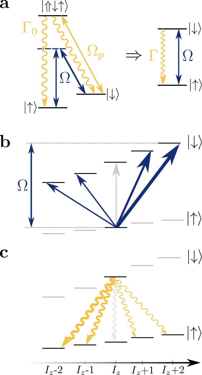
In order to reconstruct spin-state populations (and their distribution), we adapt the master equation treatment of feedback control of a nuclear spin ensemble devised by W. Yang and L. J. Sham Yang2013. Our model constitutes an extension of their work, that captures the electron-nuclear spin-flip processes enabled by the strain-induced quadrupolar interaction Urbaszek2013 : under our Raman drive, the electron spin polarisation is modulated at the Rabi frequency; this results in a time-dependent Knight field, which when driving at the nuclear Zeeman energy, enables nuclear spin-flips. The model assumes vanishing nuclear coherences and takes the approximation of Markovian dynamics. This is a reasonable approximation given that the electronic quasi-steady state in a given Overhauser field is to first order governed by the optical spin pumping (), which happens on a faster timescale than the nuclear back-action Yang2013.
The master equation governing the cooling dynamics for the nuclear density operator is:
| (26) |
Polarisation-dependent Raman scattering rates are approximated as those of a two-level system constituted by and states, as done in Hogele2012; Gangloff2019. The rate of electronic optical pumping is related to the natural linewidth of the exciton state in a lambda system, by:
| (27) |
where is the Rabi frequency of the optical pumping field (Fig. S13a). We take:
| (28) |
with:
| (29) |
being a detuning of the effective two-level drive from the transition (Fig. S13b). We have introduced as a laser detuning from the electron Zeeman splitting. The strength of pure dephasing is:
| (30) |
The decrease of polarisation fluctuations is a result of strong phase-space flow towards the state defined by the mean field where . The cooling performance is dependent on the competition of Raman scattering rates with spontaneous sideband processes and nuclear spin diffusion (Fig. S13c).
Since the system comprises multiple spin-species, we partition the mean field into the respective spin-species components:
| (31) |
each defining a species-specific nuclear polarisation.
A.2 Steady state solution
We now model the phase-space flow of the arsenic nuclear state. Here the lockpoint is set by - a component of the total mean field reconstructed from the asymmetry measurement.
Following Ref. Yang2013, we seek a steady-state probability distribution for the system to be in state , where is the number of spins in projection . This is given by:
| (32) |
which, using Eq. 26, is shown to evolve according to a rate equation:
| (33) |
with single-spin magnon-operator matrix elements:
| (34) |
and:
| (35) |
being a concise notation for a microstate accessible from through a spin-flip that changes projection of a single spin from to . In addition to the stimulated Raman scattering rates induced by the ESR drive (), spontaneous Raman scattering rates () induced by optically pumping the electron () have to be incorporated Yang2013; Hogele2012, as per Fig. S13c. At last, we account for a slow nuclear spin decay () - a thermalisation mechanism - as seen experimentally in section D. Embedding these processes in the master equation is done through the following extension:
| (36) |
The nuclear spin decay is the only process included in the master equation that allows transitions within the single-spin manifold.
Rate equation 33 has a unique steady-state solution, which is hard to find exactly in the limit. However, in this limit, treating as continuous variables is well-justified, allowing the equation to be expanded in the small parameter up to second order, which turns it into a Fokker-Planck equation Risken1984.
In doing this, it will be convenient to define functions , and a linear differential operator :
| (37) | ||||
| (38) | ||||
| (39) | ||||
| (40) |
with and . The steady-state probability distribution of the master equation, with as in the main text, is then a solution to the partial differential equation:
| (41) |
Here, all functions and their derivatives are evaluated at . To recast Eq. 41 in the more familiar form of a steady-state Fokker-Planck equation, we proceed with defining a drift vector and a diffusion tensor, with :
| (42) |
The drift terms are given by:
| (43) |
And the elements of the diffusion tensor are:
| (44) |
Finally, we use the physical constraint on populations, , to reduce the dimensionality of the Fokker-Planck equation by one. This is a straightforward exercise in multivariate calculus. In the following, we will assume that drift vector and diffusion tensor are defined in a three-dimensional space of variables , , , satisfying and .
A.3 Numerical approach to solving the problem
Setup – In this section we continue working with a single spin-species: arsenic. The lock-points of the flow are again set by - arsenic components of total mean field reconstructed from the asymmetry measurements. The objective of the following is to find a steady-state probability distribution of the state in the phase space of single-spin state populations .
As in the one-dimensional case (Fig. 1e of the main text), the drift terms in Eq. 42 lead to a sizeable feedback in the range , corresponding to a volume small compared to that of the entire phase space. This makes domain discretisation ill-suited for finding the steady-state probability distribution.
Instead, we develop a method relying on knowing the position of the centre of steady state probability distribution - . This point is found numerically by following the flow lines in the phase-space, towards a stable point that satisfies within ( locked to the Raman drive). The technique developed in this section allows to reconstruct the steady-state distribution in the vicinity of , which we a priori expect to be a sufficiently good approximation, since the strong feedback is confined to a small phase-space volume.
General method – The diffusion component of Eq. 42 scales like as compared to the drift term. This makes our case an excellent candidate for the WKB approximation Risken1984. We use the ansatz:
| (45) |
which brings Eq. 42 into the form:
| (46) |
Since this is an excellent approximation, and it reduces greatly the complexity of the problem.
Then, since is positive-definite everywhere except at the boundaries, where at least one of its components is zero, we have that at we also have . This means that the probability distribution has a local maximum at the zero of the flow field which we denoted as .
We then expand and around up to first order in :
| (47) |
Here, stands for Jacobian () and:
| (48) |
is a symmetric, Hessian matrix, which we will show to be positive-definite if is a stable point. In the vicinity of a stable lock-point, matrix defines a Gaussian probability distribution:
| (49) |
Neglecting the terms, we further reduce Eq. 46 to:
| (50) |
which is a sum of two quadratic forms. We now use the fact that for a general vector and matrix :
| (51) |
so for Eq. 50 to hold for arbitrary , the sum of symmetric matrix components of and has to be zero:
| (52) |
Provided that the zero of we identified is stable (i.e. all eigenvalues of are negative), comes out positive-definite, as desired. Note that this construction does not require to be symmetric, so it is suited for flows with non-zero curl as well (which is numerically verified to be the case in our problem).
We now outline a way to solve Eq. 52 for . We begin by multiplying by from both sides:
| (53) |
and then diagonalize and such that:
| (54) |
We then define . Finally:
| (55) |
We have now found the covariance matrix - - of the multivariate Gaussian distribution , which together with fully defines the steady-state probability distribution in the vicinity of a lock-point.
The computational complexity of arriving at this solution using our method is low. The core of the problem lies in finding numerically, which can be done by following the flow lines in the basin of attraction of the stable point. The computational cost of this procedure is comparable to that of the gradient descent algorithm. In the present case, the vector field is not a gradient of a scalar field, but its analytical form is known, and is expected to have stable zeros.
Our feedback (Eq. 33) is non-linear, and bistable, so in order to avoid convergence to the trivial solution we pick an initial guess , which corresponds to a polarisation much higher than the ones we lock the system to, and which is predicted to flow to the point by one-dimensional mean-field theory.
Entries of and are evaluated symbolically, so it is only the diagonalisation and matrix inversion that are the possible sources of numerical errors. Since the matrices involved are and real, the errors are negligible.
Solution – The covariance matrices found numerically are non-diagonal, which implies the existence of classical correlations in the optically prepared nuclear state (of a single species). A spectral analysis of these matrices shows that the eigenvector associated with the smallest eigenvalue is also a normal to the plane of constant polarisation - this is expected of the feedback mechanism designed to narrow down the fluctuations in , as highlighted in the main text.
Under the assumption of a single nuclear spin species, the electron’s inhomogeneous dephasing time predicted by the model is:
| (56) |
Thanks to the convenient form of the identified solution, fluctuations in can be calculated easily:
| (57) |
where we define :
| (58) |
as a vector decomposed in a basis of unit vectors along , and , respectively. The fluctuations of the fractional polarisation are: .
Relating the in our single-species model to the measured – How do we relate to the experimentally measured from section B? Our measured is the sum effect of all three species:
| (59) |
where we labelled the concentration of indium as .
We need to make some simple assumptions in order to connect our model value to our experimental value. Here we make two: no correlations between polarisations of species-characteristic sub-ensembles, and the same degree of fractional polarisation narrowing for each species (). Under these assumptions the model inhomogeneous dephasing time is rescaled by a factor 2 compared to the measured :
| (60) |
We note that if instead we had made the opposite assumption of correlated sub-ensembles, our scaling factor would be only different. Indeed, for sub-ensembles fully correlated by the feedback, the scales as for spins. Thus, our , which contains spins, would be of order . Most importantly, our reconstruction is insensitive to on this scale.
Fitting procedure – In order to match the model to the measured and population imbalances (Fig 3b of the main text), we leave as a free parameter in a fit, and fix the remaining parameters to the values strongly informed by previous studies on dots from the same wafer (all summarised in the Table III, at the end of the supplementary materials). Calculated values of fall in the interval.
A.4 Thermal state
We now calculate the covariance matrix that the thermal state of corresponding polarisation would feature, as per Fig. 3 of the main text.
The single-spin partition function, expressed as a function of the thermodynamic , is given by:
| (61) |
A known polarisation results in a numerically solvable equation for :
| (62) |
For a given , the probability for the single spin to have the projection is:
| (63) |
which in turn is used to calculate the thermal probability distribution following:
| (64) |
For large , we can use the Stirling approximation:
| (65) |
Then:
| (66) |
so the statistics is Poissonian, with .
In the limit of , the Stirling approximation applied to each factorial turns the Poissonian distribution into a multivariate Gaussian distribution:
| (67) |
The corresponding thermal covariance matrix is given by:
| (68) |
It features polarisation fluctuations an order of magnitude higher than those of the non-equilibrium steady state we prepare optically.
B Modelling of Gallium Polarisation (2D F-P)
While information about arsenic and indium was extracted directly from our data, we cannot draw any analogous statements on the gallium sub-ensemble due to its weaker coupling to the electron and thus its apparent absence from our magnon spectra (see Section C). However, we can intuit that the relative degree of polarisation of the two species is a function of the corresponding strength of the feedback each species experiences Yang2013:
| (69) |
To derive formally this relative degree of polarisation we use a two-species Fokker-Planck model. Without loss of generality, we treat both gallium and arsenic as spin- species. Assuming vanishing coherences, this reduces the description of the flow to the two-dimensional space of fractional polarisations spanned by and .
To estimate the co-dependence of and , we look for stable points of the flow with a lock-point set as:
| (70) |
This 2D Fokker-Planck model is analogous to the 3D case, from section A. The only difference lies in the expressions for the phenomenological Raman scattering rates, and the rates of spontaneous sideband processes, which both need to now account for the presence of the second species. The Raman scattering rates for the first and second species - , respectively - are the counterparts of the expression from Eq. 28 with the only difference lying in:
| (71) |
A similar modification enters the spontaneous sideband processes (as included in Eq. 36), where now their rate is given by:
| (72) |
Solving this 2D Fokker-Planck model uses the method already outlined in the section A for our 3D model.
Neglecting slow nuclear-spin diffusion, competition between species-characteristic sideband strengths has an effect on the covariance matrix of the steady-state probability distribution, but not its centre.
The 2-D Fokker-Planck model returns the stable points - a pair for each total Overhauser field . We connect our simulation to experimental observation by considering our simulation output over the range of experimentally observed arsenic polarisation (Fig. 4a), i.e. we simply rescale our simulation setpoint such that experimental and simulated arsenic polarisations are in the same range. In Fig. S14 we plot these stable points (solid curves), alongside the experimental data for (purple diamonds).
Over this range, the ratio of gallium and arsenic polarisation is approximately fixed. As a result, we perform linear fits of the simulations (dashed lines), and obtain (in agreement with our expectation from Eq. 69). This is the ratio mentioned in the main text.
VI Supplementary notes on steady-state coherences
Here we outline the physical mechanisms that can lead to an enhanced asymmetry of the magnon-injection processes, and show that our measurements (Fig. 4) can only be explained by a degree of entanglement among nuclei. To convey the general concept with simplicity, we will consider an ensemble of spin- nuclei ( symmetry group), in which the magnon creation/annihilation operators are simply the total angular momentum laddering operators:
| (73) |
The concepts illustrated by the model generalise straightforwardly to a high-spin ensemble interfaced with a proxy qubit. Assuming a uniform electron-nuclear coupling, the lowest type of symmetry exhibited by the system is permutation invariance. In the case of spin- systems, this leads to the conservation of total spin (a quantum number associated to the operator ), thereby partitioning the Hilbert space into sub-radiant and super-radiant sub-spaces of well defined , or - in other words - well-defined exchange symmetries Dicke1954. The proper mathematical treatment of the ensemble of permutation invariant -level systems requires working with SU() symmetry groups. Nonetheless, for permutation-invariant systems violating the conservation of momentum (like the ensemble considered in the manuscript), the conservation of exchange symmetry still holds. As a result, the physical mechanism of many-body interference, destructive or constructive interference, leads to analogous quantum phases of the ensemble: sub-radiant and super-radiant.
.1 General entanglement witness
Taking an ensemble of spin- particles, the following inequality holds for any separable state:
| (74) |
where is the variance of collective operator ; violation of this bound implies entanglement Vitagliano2011.
.2 Asymmetry parameter as an entanglement witness
In this general quantum picture, the magnon exchange frequencies are correlators of collective spin operators :
| (75) |
This expectation value is correct for any many-body state, quantum or classical. The asymmetry parameter, as we measure it, is simply a ratio of these correlators, where we use and to denote the commutator and anti-commutator respectively:
| (76) |
This is then expressed as expectation values of the collective spin operators :
| (77) |
The asymmetry parameter is then simply a ratio of longitudinal first moment of polarisation to transverse second moments of polarisation:
| (78) |
We then use the relation between variance and second moments to solve for the noise terms as a function of asymmetry:
| (79) |
Now using the general entanglement witness, Eq. 74, we can express the asymmetry parameter as a formal entanglement witness:
| (80) |
This expression can be recast in terms of mean fractional polarisations , where for spin-, and the asymmetry-commensurate longitudinal fractional polarisation :
| (81) |
Violation of this general inequality then necessarily implies the presence of entanglement in the spin ensemble.
.3 Universal features
While Eq. 81 was derived for a spin- ensemble, certain universal features can be extracted that only depend on fractional polarisations and are independent of the spin character of the ensemble:
- •
In any system, the entanglement condition is inversely proportional to transverse coherences ; i.e. entanglement is present at lower values of for a state with transverse coherences.
- •
In a system where the longitudinal fluctuations are highly sub-thermal, , Eq. 81 becomes:
(82) which necessarily implies that the following observation is sufficient to prove the presence of entanglement:
(83)
.4 Experimental observations
Our experimental observations are that the nuclear ensemble following optical preparation has longitudinal fluctuations (measured in section B as the electronic ) reduced by a factor of relative to their thermal value Ethier-Majcher2017; Gangloff2019, i.e. . We have no direct measurement of transverse coherences , however we have shown that such coherences would reduce the asymmetry for which the state remains classical. Our measurements shown in Fig. 4 reveal that for our nuclear state, summed over species, . In other terms, the asymmetry-commensurate polarisation , averaged over species, exceeds the underlying fractional polarisation by a factor of , well beyond the bound set out by Eq. 83 .
The quantum picture introduced in section .2 prompts us to evaluate separately the numerator and the denominator of our sideband asymmetry parameter (c.f. Eq. 78). The numerator is directly proportional to a longitudinal population difference up to a factor that is independent of the nuclear wavefunction symmetry. The denominator, on the other hand, directly reflects the transverse noise. We therefore show these quantities as experimentally measured (Fig. S15). These data show that the longitudinal population difference changes linearly with polarisation (), whereas the transverse noise () remains constant within experimental noise. We thus conclude that the optical preparation of the nuclear ensemble not only reduce longitudinal fluctuations by a factor of , but it also suppresses transverse fluctuations by a factor of , and that this fluctuation reduction is independent of polarisation.
.5 Sub-radiance
We can re-express the asymmetry parameter, Eq. 78, as function of total angular momentum , and for a reduced fluctuation state for which :
| (84) |
The enhancement of asymmetry to , i.e. beyond that featured by a low-polarisation product state (which is , is a signature of:
| (85) |
characteristic for a dark state, as it implies even for small . It is instructive to consider the opposite limit, where:
| (86) |
In such case, for states of the asymmetry is decreased close to zero.
These insights allow the introduction of a phase diagram (Fig. 4b inset) showing vs. where, in the case of a longitudinally narrow state , deviation from the one-to-one classical line (no coherences), , can indicate the dominant type of interference (constructive or destructive).
VII Summary of model parameters
| Total hyperfine interaction, arsenic, | |
|---|---|
| Total hyperfine interaction, indium, | |
| Total hyperfine interaction, gallium, | |
| Indium concentration , x | |
| External magnetic field, | |
| Arsenic Zeeman splitting, | |
| Indium Zeeman splitting, | |
| Gallium-69 Zeeman splitting, | |
| Gallium-71 Zeeman splitting, | |
| Inhomogeneous dephasing time, |
| Electron homogeneous dephasing time, | |
|---|---|
| Electron Rabi frequency in asymmetry measurement, | |
| Pure dephasing timescale for arsenic sideband transitions, | |
| Pure dephasing timescale for indium sideband transitions, |
| Arsenic quadrupolar angle, | |
|---|---|
| Rabi frequency, | |
| Trion linewidth, | |
| Effective optical pumping rate, | |
| Number of arsenic Nuclei, | |
| Electron homogeneous dephasing time, | |
| Arsenic quadrupolar constant, | |
| Arsenic spin diffusion rate, |
References
- (1) Bodey, J. H. et al. Optical spin locking of a solid-state qubit. npj Quantum Inf. 5, 95 (2019).
- (2) Stockill, R. et al. Quantum dot spin coherence governed by a strained nuclear environment. Nat. Commun. 7, 12745 (2016).
- (3) Éthier-Majcher, G. et al. Improving a Solid-State Qubit through an Engineered Mesoscopic Environment. Phys. Rev. Lett. 119, 130503 (2017).
- (4) Huthmacher, L. et al. Coherence of a dynamically decoupled quantum-dot hole spin. Phys. Rev. B 97, 241413 (2018).
- (5) Gangloff, D. A. et al. Quantum interface of an electron and a nuclear ensemble. Science 364, 62–66 (2019).
- (6) Urbaszek, B. et al. Nuclear spin physics in quantum dots: An optical investigation. Rev. Mod. Phys. 85, 79–133 (2013).
- (7) Jackson, D. M. et al. Quantum sensing of a coherent single spin excitation in a nuclear ensemble. Nat. Phys. (2021).
- (8) Gillard, G. et al. Fundamental limits of electron and nuclear spin qubit lifetimes in an isolated self-assembled quantum dot. npj Quantum Inf. 7, 43 (2021).
- (9) Wüst, G. et al. Role of the electron spin in determining the coherence of the nuclear spins in a quantum dot. Nat. Nanotechnol. 11, 885–889 (2016).
- (10) Wiener, N. Extrapolation, Interpolation, and Smoothing of Stationary Time Series, with Engineering Applications (Martino Fine Books, 2013).
- (11) Bulutay, C. Quadrupolar spectra of nuclear spins in strained In xGa 1-xAs quantum dots. Phys. Rev. B - Condensed Matter and Materials Physics 85, 115313 (2012).
- (12) Yang, W. & Sham, L. J. General theory of feedback control of a nuclear spin ensemble in quantum dots. Phys. Rev. B 88, 235304 (2013).
- (13) Högele, A. et al. Dynamic Nuclear Spin Polarization in the Resonant Laser Excitation of an InGaAs Quantum Dot. Phys. Rev. Lett. 108, 197403 (2012).
- (14) Risken, H. Fokker-Planck Equation, 63–95 (Springer Berlin Heidelberg, Berlin, Heidelberg, 1984).
- (15) Dicke, R. H. Coherence in spontaneous radiation processes. Phys. Rev. 93, 99–110 (1954).
- (16) Vitagliano, G., Hyllus, P., Egusquiza, I. L. & Tóth, G. Spin Squeezing Inequalities for Arbitrary Spin. Phys. Rev. Lett. 107, 240502 (2011).