Improving J-divergence of brain connectivity states by graph Laplacian denoising
Tiziana Cattai1,2,3, Gaetano Scarano3, Marie-Constance Corsi1,2, Danielle S. Bassett4,5,6,7,8,9 Fabrizio De Vico Fallani1,2, Stefania Colonnese3
1 Inria Paris, Aramis Project Team, Paris, France
2 Institut du Cerveau et de la Moelle epiniere, ICM, Inserm U 1127, CNRS UMR 7225, Sorbonne Universite, Paris, France
3 Dept. of Information Engineering, Electronics and Telecommunication, Sapienza University of Rome, Italy
4 Department of Bioengineering, University of Pennsylvania, Philadelphia, PA, 19104, USA
5 Department of Electrical and Systems Engineering, University of Pennsylvania, Philadelphia, PA, 19104, USA
6 Department of Physics & Astronomy, University of Pennsylvania, Philadelphia, PA, 19104, USA
7 Department of Neurology, Hospital of the University of Pennsylvania, Philadelphia, PA, 19104, USA
8 Department of Psychiatry, Hospital of the University of Pennsylvania, Philadelphia, PA 19104, USA
9 The Santa Fe Institute, Santa Fe, NM, 87501 USA
Corresponding author: tiziana.cattai@uniroma1.it†† This work has been submitted to the IEEE for possible publication. Copyright may be transferred without notice, after which this version may no longer be accessible
Abstract
Functional connectivity (FC) can be represented as a network, and is frequently used to better understand the neural underpinnings of complex tasks such as motor imagery (MI) detection in brain-computer interfaces (BCIs). However, errors in the estimation of connectivity can affect the detection performances. In this work, we address the problem of denoising common connectivity estimates to improve the detectability of different connectivity states. Specifically, we propose a denoising algorithm that acts on the network graph Laplacian, which leverages recent graph signal processing results. Further, we derive a novel formulation of the Jensen divergence for the denoised Laplacian under different states. Numerical simulations on synthetic data show that the denoising method improves the Jensen divergence of connectivity patterns corresponding to different task conditions. Furthermore, we apply the Laplacian denoising technique to brain networks estimated from real EEG data recorded during MI-BCI experiments. Using our novel formulation of the J-divergence, we are able to quantify the distance between the FC networks in the motor imagery and resting states, as well as to understand the contribution of each Laplacian variable to the total J-divergence between two states. Experimental results on real MI-BCI EEG data demonstrate that the Laplacian denoising improves the separation of motor imagery and resting mental states, and shortens the time interval required for connectivity estimation. We conclude that the approach shows promise for the robust detection of connectivity states while being appealing for implementation in real-time BCI applications.
1 Introduction
Functional connectivity describes how brain areas mutually interact [1]. This information can be modeled as a graph, which is one of the most common formalism to characterize networked data [2, 3]. Many recent studies prove that mental states can be characterized by graph statistics, such as node strength, efficiency, and modularity [4]. Detecting brain connectivity-related features corresponding to different mental states can enhance several technologies, such as brain-computer interfaces (BCIs). BCI systems allow subjects to communicate and interact without peripheral neuro-muscular activity [5]. The requirement for the BCI functioning is therefore the correct detection of the user’s mental states. While research on the subject has significantly advanced over the last decade, there is still a key limitation known as BCI inefficiency [6]. It refers to the fact that there is a percentage of users who cannot be trained to use the interface. This limitation, together with system-user interaction problems [6], motivated us to develop new tools with the intent of having a more robust estimate of brain connectivity with the final goal of better separating two cognitive states. Implementing this estimate from signals acquired at graph nodes (e.g. EEG electrodes) is a difficult task because of the inherent noise, the number of links to estimate, the presence of artifacts, the non-stationarity of the signal.
To address the problem of connectivity estimation together with the improvement of separability between mental states to optimally control a BCI, it is necessary to combine tools from different fields, such as neuroscience and signal processing. For example, graph signal processing (GSP) can be applied in this scenario [7, 8, 9]. GSP has already been used to deal with biological data, and in particular brain data [10, 11]. Indeed, GSP is potentially able to integrate information regarding brain structure, as represented by the graph itself, with information regarding brain function, as represented by the graph signals.
Another helpful tool to the brain connectivity estimation problem is the signal detection theory. Detection procedures can be applied to investigate statistical differences between the brain connectivity features of two different mental states, which corresponds to motor imagery and resting state for our applications. In this context, widely adopted statistics are the Likelihood Ratio (LR) of the features [12, 13, 14, 15, 16, 17, 18, 19] as well as the linear detector maximizing the so-called deflection [20, 21, 22, 23]. With the aim of obtaining a distance metric of features under two states, the case of normally distributed observations simplifies the analysis. Indeed, for normally distributed observations with equal conditional variance and different conditional means, the maximum deflection test coincides with the LR test. Moreover, this latter can be extended to a linear quadratic detector so as to cope with observations characterized by different conditional variances. [20, 21]. To obtain a measure of separability between features under the two states, one possibility is the Jensen divergence which reflects the maximum deflection test performance [12, 19, 14].
In the following sub-section, we present our original contributions.
Paper Contributions
- •
This paper proposes a novel graph Laplacian denoising algorithm, to enhance the accuracy of brain connectivity estimates. In recent literature, several studies have been conducted to improve the accuracy of link estimation, whereas few studies approach this problem in terms of description of the graph algebraic structure (see Section 2). We address this limitation by proposing a subspace-based Laplacian denoising algorithm that preserves relevant connectivity features while rejecting noise-dominated components. In particular, the Laplacian denoising preserves i) the sub-spaces more directly related to the graph topology, as summarized by the eigenvectors corresponding to the smallest Laplacian eigenvalues, and ii) the sub-spaces estimated under a favourable signal-to-noise ratio, as summarized by the eigenvectors corresponding to the largest Laplacian eigenvalues. The noise rejection obtained by this twofold sub-space selection notably improves the separability of two connectivity states. To sake of clarity, we refer to connectivity states as the patterns of connectivity estimated while the brain performs distinct cognitive tasks.
- •
In order to measure the improvement achieved by the proposed brain connectivity denoising algorithm, we provide an analysis of the J-divergence of the Laplacian coefficients, we explicit their contribution to the states’ separability in terms of their first and second order moments of the test statistics, and we show that the proposed Laplacian denoising actually increases the J-divergence of the brain connectivity features rest (null) or motor imagery (alternative). The improvement of the J-divergence of the graph Laplacian coefficients under different connectivity states is assessed by numerical simulations on synthetic data.
- •
Finally, we present experimental results on real EEG data acquired during motor imagery-based BCI experiments, and we prove that the proposed novel denoising algorithm increases the J-divergence of brain connectivity states and paves the way for connectivity estimation time interval reduction. As a relevant by-product of the theoretical J-divergence analysis, we are able to attribute a score to each and every Laplacian coefficient representing its marginal contribution to the J-divergence. The score admits relevant biological interpretation confirming the efficacy of the approach. These results can be assessed by further studies on the brain connectivity features.
The structure of the paper is as follows. Section 2 reviews the scientific literature related to our work. Section 3 describes the signal model used in the analysis. Section 4 details the novel graph denoising we propose. Section 5 describes the problem of Gaussian detection, and it presents the novel formulation of J-divergence we use throughout the paper. In section 6, we test our filtering method on synthetic graph to verify its ability to separate two graphs. Section 7 applies our method on real EEG data, exhibiting its capacity to estimate graph connectivity during motor imagery tasks and to discriminate between two mental states. We conclude in section 8. In Table 1, we list of the main notation used in the paper.
| Notation | Description |
|---|---|
| , | adjacency matrix (real, estimated) |
| V | set of all nodes |
| N | total number of nodes |
| E | set of all links |
| , | degree matrix (real, estimated) |
| , | Laplacian matrix (real, estimated) |
| , | eigenvalue (real, estimated) |
| , | eigenvector (real, estimated) |
| , , | subset of smallest, central, larger eigenvalues |
| , | filtered graph laplacian matrix and vector |
| transformation matrix | |
| vectorized laplacian in the transformed domain | |
| J | J-divergence |
| score |
2 Related Work
The problem of graph connectivity estimation has been well studied in literature in different domains, from neuroscience to signal processing and graph theory [24, 25, 26]. State-of-the-art graph learning methods have the limitation that they usually present over-simplified models for the signal on graph to overcome problems of computational and memory cost. Some recent works, such as [27], propose different strategies to deal with graph learning problems. Specifically, in the context of mental state identification, authors in [27] present a novel technique to create and modify embeddings associated to each graph node to efficiently compute the adjacency matrix. Since FC computation requires a lot of time and computational power, one possibility consists in clustering FC into relevant communities of synchronous components. One approach, recently proposed in [28], goes in this direction with the application of k-means clustering algorithm followed by a tensor decomposition to reduce the FC data.
FC estimation can leverage the generalization of classical signal processing operations into the graph setting, where signals are localized on graph nodes, giving rise to novel research domain of the graph signal processing (GSP) [9, 7, 8]. GSP has already showed its potential to describe brain functioning in [29] and [10]. Indeed, GSP representation naturally fits to the brain, where the structure can be described by the graph itself while brain functioning directly corresponds to graph signals. An interesting application is graph filtering [7, 30] which can be useful to extract meaningful brain behaviour [31]. In [32], authors propose a mathematical model for brain fibers able to describe neurophysiological mechanisms. The model, based on GSP techniques, extracts a subset of graph eigenvectors which represent a suitable basis for filtering fiber tracts from brain imaging data.
GSP techniques have been applied also to brain-computer interfaces with NIRS signals [33]. Specifically, GSP analysis is leveraged in [33] in the context of feature extraction to extract spatial information from the NIRS signals and it has been shown to improve classification performances.
Classical signal processing techniques and eigenvector-based filtering have already been used with brain data [34, 35]. In [36] and [37], eigenvector-based filters are applied to fetal magnetic signals and diffuse optic imaging data to obtain more localized activities and reduce artifacts and noise. Specifically, in [37], classical eigenvector-filtering, i.e. based on larger eigenvectors, is used in diffuse optical imaging with the aim to improving connectivity estimation.
In the following, stemming from the GSP approach to FC estimation, we propose a novel Laplacian denoising algorithm, and we show that it improves the statistical separation of distinguished connectivity states. To this aim, we provide an analysis of the J-divergence, which naturally provides a metric to quantify the distance between two distributions, for the problem under concern. Recently, the J-divergence has been applied in [38] to investigate the time series’ irreversibility . Another recent application of the J-divergence is proposed in [39], where authors present a novel approach to vector-skew the J-divergence. This method is able to preserve J-divergence properties and simultaneously to fine tune parameters for specific applications.
J-divergence has been also applied in the context of BCI design, to tackle one of the most challenging issues of EEG-based BCIs, which is the long calibration time. In general, the number of data required to calibrate the model is really high, because of the noise and the non-stationarity of brain signals. One solution comes from [40], where a subject-to-subject transfer learning is proposed to improve the classification performance with limited training data. J-divergence is used in a transfer learning framework to test their method by comparing the data of the target subject with the data from previous subjects. In the following, we investigate the J-divergence under a different points of view, namely i) we assess the performance of the denoising algorithm in separating connectivity states and ii) we provide criterion for scoring the Laplacian coefficients based on their contribution to the connectivity states separation.
3 Signal Model
We are interested in analyzing signals defined on an undirected, connected, weighted graph , which consists of a finite set of vertices V with , a set of edges E and a weighted adjacency matrix A. If there is an edge connecting vertices i and j, the element represents the weight of the edge; otherwise, .
The graph Laplacian, is a real symmetric matrix defined11 1 We refer here to the non-normalized graph Laplacian, also called the combinatorial Laplacian. as:
| (1) |
where the degree matrix is a diagonal matrix whose diagonal element is equal to the sum of the weights of all the edges incident to vertex . We denote by set of orthonormal eigenvectors, corresponding to increasingly ordered eigenvalues .
In GSP, the Laplacian eigenvectors are considered as SoGs and provide a basis for the Graph Fourier Transform. For a SoG s, the GFT is defined as the projection of s on the eigenvectors of the graph Laplacian: . The graph Laplacian eigenvalues have an analogous meaning to Fourier transform frequency, i.e. smaller eigenvalues are associated to eigenvectors that exhibit smoother variations over connected nodes.
In many SoG application problems, including brain functional connectivity estimation, signal values are actually represented by discrete sequences, obtained by sampling a continuous time signal at each graph node.
Let us denote the sequences of samples acquired over an observation period with sampling pace as , , or in vector form as The vector sequence is used to estimate the graph adjacency matrix by computing a similarity metric on each and every node pair. There are many state-of-the-art methods to estimate , which associate link weights according to different interaction properties [1, 41, 42, 43]. Thereby, the adjacency matrix is actually represented by its estimated version , which contains the connectivity values estimated for each graph node pair . Accordingly, the estimated degree matrix is computed, so as to derive the estimated laplacian through Eq. 1, that becomes here:
| (2) |
Any estimation error on the adjacency matrix affects the Laplacian estimate, and it results into less distinguishable connectivity states. In the following section we address the denoising of the estimated Laplacian for the purpose of improving the separation of connectivity states.
4 Graph Connectivity Denoising
In order to introduce the Laplacian denoising algorithm, we consider the eigenvalue decomposition of the estimated Laplacian matrix as follows:
| (3) |
Perturbations affect graph Laplacian estimation in terms of both eigenvalues and/or eigenvectors. To elaborate on the effect of perturbations, we explicit the first, second and third order error contributions to the estimated laplacian as:
| (4) |
Thereby, the estimated Laplacian can be approximated at the first order as the sum of terms:
| (5) |
Eq.(5) highlights the first order error contribution due to relative perturbation of the Laplacian eigenvalues as well as of the eigenvectors direction. We are interested in the Laplacian components whose perturbation is contained because either the relative eigenvalue perturbation or the eigenvector perturbation is (relatively) small. To this aim, we order the set of orthonormal eigenvectors with increasingly eigenvalues , and we consider three subsets of eigenvalues and associated eigenvectors: the subset containing the smallest eigenvalues; the subset containing the largest eigenvalues; and the subset containing the remaining central eigenvalues, with .
Firstly, we remark that the largest eigenvalues are more robust to eigenvalue perturbation; this assumption is usually exploited in classical signal processing, where the subspace is used for the estimation of the covariance matrix because of its favorable signal-to-noise ratio [44].
Secondly, stemming on recent literature results [45], it can be expected that the subspace is partially robust in terms of eigenvector perturbation. In fact, in [45] the authors states that a connectivity estimation error on the adjacency matrix element, i.e. on the weight of the link between the -th and the -th nodes, induces a perturbation of the -th eigenvector depending on the difference between the -th and the -th coefficients of . Thereby, eigenvectors smoothly varying across the -th and the -th nodes are less affected by estimation errors on . On the other hand, in GSP, it is well known that eigenvectors, corresponding to small eigenvalues, represent low frequency basis elements in the Graph Fourier Transform [46],[9] since they are characterized by the smallest variations across strongly connected graph regions. Thereby, the eigenvectors in are equipped with inherent resilience to connectivity estimation error within these regions. On the other hand, the eigenvectors in are tightly related to the network connectivity, and therefore they need to be involved in the devised denoising method.
Stemming on these observations, we propose a denoising method based on preserving the contribution to the Laplacian due to the subspaces , while discarding those relative to the subspace . In formulas, given the estimated Laplacian
| (6) |
we compute the denoised Laplacian as follows:
| (7) |
We recognize that the proposed, subspace-based, Laplacian denoising approach allows preservation of
- •
the sub-space , which is directly related to the graph connectivity features
- •
the sub-space , which is estimated with a favourable signal-to-noise ratio.
The proposed Laplacian denoising method, synthetically presented in Algorithm , preserves the information relevant for the purpose of graph connectivity identification, while rejecting noisy components. In order to quantify the improvement achieved in terms of connectivity state separability, we resort to the J-divergence as a metric of the distance between connectivity states. In the following we derive a formulation the J-divergence for the problem under concern.
5 Jensen divergence of connectivity states
Several metrics can be adopted to determine the separability of two connectivity states [47], as represented by the Laplacian matrix . Herein, we resort to the notion of J-divergence for characterizing the separability of connectivity states, and we reformulate it for the problem under concern. Thus, J-divergence is used to identify the Laplacian coefficients that are most relevant for detection purposes and later on to measure the improvement achieved by the proposed denoising algorithm.
For the purpose of the analysis, we will assume that the Laplacian coefficients obtained at the output of the denoising algorithm are normally distributed. Let us remark that the Gaussian assumption stands in many applications22 2 The reason why this occurs is that the Gaussian assumption tightly models laplacian diagonal elements, computed in each row as the sum of extradiagonal elements in that column, as well as extradiagonal elements which are often computed as the result of correlation estimates., including the case of connectivity estimates carried out on real brain signals, and thereby it is often assumed in the literature, e.g. for Laplacian estimation purposes [7]. Specifically, we assume that the vector is distributed according to a multidimensional Gaussian probability whose mean vector and covariance matrix differ under two different connectivity states, referred to as the null and the alternative hypotheses , in the following: 33 3 The notation , with indicates that the random vector is Gaussian distributed with mean vector and covariance matrix .
| (8) |
As an information theoretic measure of distance between under and , we now compute in analytical form the J-divergence, which is defined as the expected value of the difference of the Log Likelihood Ratio under the two hypothesis and [14]. The J-divergence formulation will allow us to evaluate to which extent the connectivity states represented by the Laplacian coefficients are distinguishable from each other.
Let us first assume that the Laplacian moments ,,, are known. Detection can then be conducted on a linear transformation of the observations:
where and is an affine transform that simultaneously44 4 The matrix and the diagonal matrix are computed as the generalized eigenvectors and the generalized eigenvalues matrices of the pencil , respectively. Given any square root of , i.e. such that , we may conveniently employ the unitary transformation obtained from the eigenanalysis ; in fact, it is easily proved that the matrix verifies with . whitens the observations in the hypothesis obtains uncorrelated observations in the hypothesis. An example of the action of the transform , is shown in Fig. 1 for the case of -dimensional Gaussian data whose mean and covariance matrix differ under the . The original data points are plotted in Fig. 1(a), whereas their transformed counterparts are represented in Fig. 1(b). The transformed data are unitary variance, zero-centered under and are uncorrelated under .

In real detection systems, the moments can be either estimated from a training set, e.g. during a BCI training phase, or coarsely initialized and tracked throughout the system life, using methodologies, priors, and heuristics related to the application-specific problem under concern [48, 49, 50]. Besides, the transformed data can be obtained even avoiding computation of the moments and of , by applying the laplacian coefficients to a suitably trained network [51], that will enforce the afore-mentioned statistical constraints.
With these position, the observation model becomes:
| (9) |
The J-divergence is then defined as:
| (10) |
being the Log-Likelihood Ratio55 5 The Log-Likelihood Ratio is widely adopted classical LLR detection: , being selected according to the desired detection versus missing probability tradeoff.:
| (11) |
Let us now associate the variables whose variance to the first indexes and the remaining ones to the indexes 66 6 Possibly, we might have or . so as to rewrite the LLR as follows:
| (12) |
By adding and subtracting the term we rearrange the summation (12) as:
| (13) |
The variates , having different conditional variances under the hypotheses , contribute to the LLR by the terms quadratic terms. The variates , having equal unitary conditional variances under the hypotheses , contribute to the LLR by the linear terms. To gain further insight on the J-divergence, we resort to the following theorem, whose demonstration is reported in the Appendix.
Theorem 1
Theorem 1 generalizes the result in [13, 14] where only the case of variables having equal conditional means and different covariances (i.e. ) has been addressed.
The J-divergence as formulated in Eq.(15) is a measure of the statistical distance of the graph Laplacian coefficients under two connectivity states and , and it will be used to quantify the improvement of separability of brain connectivity states achieved by the denoising algorithm described in section 4.
Furthermore, the above analysis sheds a light upon the variables that mostly contribute to the states separability. From Eq.(15), we see a one-to-one correspondence between the transformed space variables and the terms of the J-divergence ; besides, the term can be of two kinds
| (16) |
depending on whether the variable changes both in conditional mean and standard deviation, or in conditional mean only. The functions are plotted in Fig.2 for between and and from to .

Interestingly, in Fig.2 we recognize that a conditional variance change gives a higher contribution to than an equal conditional mean change.
To sum up, the above analysis highlights the contribution of each of transformed variable to the separability of the connectivity states, and allows to rank their relevance to , so as to identify the transformed variables which mostly differ under the two hypothesis. This paves the way for an information theoretic scoring of the Laplacian coefficients, described in the following.
5.1 J-Divergence based Laplacian coefficients scoring
As a by-product of the analysis, we are now able to identify which Laplacian coefficients (i.e. links weights or nodes degrees), contribute mostly to the connectivity states separability. This is obtained by attributing a score to the Laplacian coefficients measuring their contribution to the J-divergence .
By definition, the Laplacian coefficient , contribute to each transformed variable . Thereby, we introduce a score , evaluated by suitable backpropagation of the terms on each contributing Laplacian coefficient. Specifically, the -th coefficient score is computed as
| (17) |
where we recognize that the weight representing the contribution of the -th Laplacian coefficient to the -th transformed variable is normalized with respect to the sum of the weights of all the contributing coefficients.
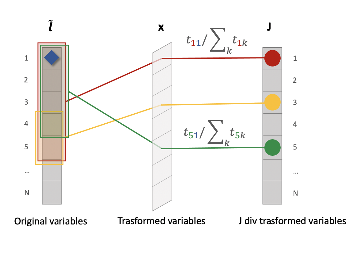
A graphical interpretation of the score is provided in Fig.3, where we represent the set of variables belonging to the original domain (left), the set of variables belonging to the transformed domain (center) and the corresponding marginal contributions to (right). The relationship between and is given by the transformation matrix that blends variables from the original domain to the transformed one. Each J-divergence component (colored circle on the right) is associated to the variable in the transformed domain, which in turn is originated by many (shaded colored box on the left). Thereby, is backprojected to the original domain by weighting its contribution as in Eq. 17. Back-projection and accumulation can also be applied by limiting the summation in Eq.(17) to the largest ranking terms. The score computation allows to quantify the relevancy of the Laplacian coefficients for state separability, and in the experimental results we show that it leads to meaningful results in case of real BCI data. The Algorithm review the main steps of the J-divergence computation and scoring procedures.
Input: Estimated Laplacian
Output: Denoised Laplacian
Input: Conditional means , and covariance matrices , of under and
Output:
6 Results on synthetic data
In this section, we test the performance of the Laplacian denoising presented in section 4 in improving the J-divergence of two estimated connectivity states over synthetic SoGs. To this end, we first consider a graph and a model for signals at nodes under two connectivity states, selected to represent an over-simplified model of brain EEG signals functional connectivity; real brain signals are considered in the next section.
We compare our approach with the case of laplacian without filtering (that we refer as and with several of eigenvector-based filters, i.e. , ). Then, we explain in detail the analysis we performed and the related results.
6.1 Signal on Graph generation and connectivity estimation
In order to validate our framework on synthetic data, we define signals under the two hypothesis and to obtain two distinct graph connectivity states.
Under , we model the network activity by considering scalar generator signals . Each generator signal simultaneously contributes to the signals measured over a subset of nodes identified by the non-zero component of the binary vector . A noise component and a common component across all the nodes are also present. Under , only these latter components are observed. With these positions, we come up with the following expression for the vector of the observed signals under the two hypothesis and :
| (18) |
In the simulations, the noise is a realization of a discrete, stationary, white Gaussian process, with ; the samples of discrete sequences are realizations of a zero mean Gaussian random distribution with variance ; and are drawn from a zero mean unit variance Gaussian random variable.
Once SoGs samples are obtained, we estimate the adjacency matrix. There are many state-of-the-art methods to perform the estimation, such as spectral coherence [42], imaginary coherence [43], phase-locking value which differently characterize brain interactions [52]of the signals at two nodes as:
| (19) |
In Eq. (19), , and are the the estimated auto-spectra and cross-spectrum of the signals , at the nodes and , computed at the frequency bin77 7 All the power spectral estimates are computed with Welch method, with s length Hanning windows and overlap of . . Given as in Eq. (19), the adjacency matrix ,estimated is averaging across the frequency bins as follows:
| (20) |
To sum up, our proposed signal model for synthetic data determines a simple graph connectivity under the two hypotheses and . The model successfully reproduces a network characterized by distinguishable connectivity states in presence of controlled perturbations. In Fig. 4, the estimated adjacency matrix is plotted under the two conditions and in presence of perturbations. We recognize that under there are no links and fluctuates around zero because of the perturbations. Under some connections exist but their values are affected by the perturbations.

Once we have obtained the adjacency matrix estimations under and , we compute the estimated Laplacians as in Eq. (2) and then, we decompose it with its eigenvalues and eigenvectors as in Eq. (3). In order to recall the eigenvectors’ behaviour, we plot in Fig. 5 the first and the eigenvectors on graph under hypothesis. We can see that the first eigenvector, in Fig. 5(a) perfectly appears smooth on the graph and within a subset of linked nodes. Fig. 5(b) describes the eigenvector on graph. Here, the eigenvector is mostly smooth, it highlights another community, but it shows higher variability than the first eigenvector over linked nodes.

This model will be used to test the proposed Laplacian denoising algorithm. To this goal, we randomly produce repetitions (or trials) for each statistical hypothesis, as i.i.d. realizations of our model with a fixed set of parameters. Different noise and polarization level will be considered.
6.2 Sub-space robustness on synthetic data
In this sub-section, we compare our laplacian-based filtering based on , shortly denoted as , with , and . Specifically, we investigate the robustness of the different sub-spaces with simulated data.
With the final goal of measuring the sub-space robustness, for each sub-space we take into account two cases, namely the absence and the presence of perturbation, to which we refer to as the ground truth (GT) and the noisy cases, respectively. Each ground truth sub-space is compared to different noisy cases, corresponding to for noise and for polarization. To quantify sub-space robustness on synthetic data, we firstly measure the Frobenius subspace distance [53] between the GT case and the noisy configurations, varying the perturbation levels88 8 For each sub-space configuration, we compute the Frobenius distance between its noisy and GT versions. See Definition 2 in [53] for the mathematical formulation.. Results of this analysis are in Fig. 6. We plot versus the trial for the subspace (red), the subspace (green), and the subspace (blue) in several perturbation conditions. In Fig. 6(a) we have the zero perturbation case, in which, not surprisingly, for every filter and every trial. With a gradual increase of perturbations (i.e. noise only case in Fig.6(b) or polarization only case in Fig.6(c)), the most favorable case is with for almost every trial. When perturbations dramatically increase Fig.6(d), performances decrease in particular for filter. In this figure, we do not report results for case because for all the trials with all the eigenvectors.

It is then clear that the eigenvectors in are significantly robust. This is not surprising, since in classical signal processing larger eigenvectors are used because of their advantages in signal-to-noise-ratio (SNR). Still, the subspace maintains the robustness, while being relevant to describe the inherent topology of the graph. In the next results, we show that the Laplacian denoising leveraging the subspace leads to better distinguishable connectivity states in absence and in presence of perturbation.

6.3 J-divergence computation on synthetic data
Finally, we test the ability to separate graph Laplacians under the hypotheses and . The J-divergence analysis presented in section 5 ends with a measure of the statistical distance between two states. Here, the analysis of separability between two states is applied to graph laplacian in simulated scenario with the goal of comparing the discriminant ability of our denoising method with respect to the other sub-space configurations, i.e. , and .
Here the two conditions are the two hypothesis and and we perform simulations for several perturbation levels. In every case, we compute the total as a measure of statistical distance between the two conditions and we also evaluate the marginal as measure of the contribution of each n-variable to the final separability. Table 2 collects J-divergence values for several perturbation sets and for different sub-spaces. Results show that in absence of perturbations the most favorable case is . This result is intuitive because in absence of perturbations there is no reason why reduced sub-spaces should better discriminate. Interestingly, increasing perturbations (i.e. noise and polarization), the most favorable case is , which gives the highest , i.e. the best separability. It means that graph laplacian denoising through preserves the highest separability between the two hypothesis, even in presence of strong perturbation. Fig 7, shows behavior as function of the first variables only for and cases. These representations make clear the contribution of variables to the final . From Fig 7 we recognize that increasing perturbations, variables in generally give higher contributions compared to .
![[Uncaptioned image]](2012.11240v2/table_jdiv_sim_01.png)
Our results with synthetic data show that in presence of perturbations our laplacian filtering succeeds in distinguishing graphs under two conditions. This conclusion remains true if the system is perturbed by noise but also if there is an artefact of different nature, i.e. a common artifact that we indicated as polarization and which can represent real phenomena.
7 Real BCI measurements
In this section, we present experimental results of our graph laplacian filtering on real data, recorded during motor-imagery BCI experiments. In this case the and hypothesis directly correspond to he hypothesis that subject performs motor imagery () or he/she is in resting state ().
7.1 Experimental Protocol and Preprocessing
The study was conducted on twenty healthy subjects (aged years, women), all right-handed. All the subjects, which did not present any disorder, received financial compensation for their participation and they signed a written informed consent. The ethical committee CPP-IDF-VI of Paris approved the experimental protocol. During the BCI experiments, every subject was in front of a screen with a target. Subjects were instructed to perform right hand - motor imagery task when the target was up, while remaining at rest when the target was down [54]. A -channel system was used to record EEG data in a standard - configuration. The reference for EEG were set to mastoid signals; the ground electrode was located on the left scalpula; and impedences were lower than 20 kOhms. Sampling frequency for EEG recordings was 1 kHz, and then downsampled to 250 Hz. For each subject, recorded sequences have been segmented to obtain trials of motor imagery and trials of resting state. The total length of each trial was s.
7.2 J-divergence of brain connectivity states
Here, we perform the J-divergence analysis on real motor-imagery data. To this aim, we take EEG signals from one subject and trials for and trials for , with . We use spectral coherence to build the connectivity matrix, as in Eq. (19). Then, the estimated adjacency matrix is computed as in Eq. (20), and thanks to the Eq. (2), we can derive . As for synthetic data, we compute the filtered graph laplacian with the subset . We compare results on real data with , , . In each case, we compute J-divergence as in Eq. (10) and the marginal contribution associated to the -th variable as in Eq.(15).
![[Uncaptioned image]](2012.11240v2/table_J_real_allfreq.png)

In Table 3, we report J-divergence results for each sub-space configuration. Comparing all the methods, the highest value relates to case. This result is very important because it means that the sub-space is suitable to separate real EEG data and it is useful to correctly detect the subject mental state.
With the aim of understanding the contributions of different variables, we firstly compute the marginal contributions to obtain a weight to each variable in the transformed domain. Then, we compute the cumulative sum of the first variables. Once the vector is sorted, we evaluate the cumulative J-divergence to investigate the impact of the variables to the total J-divergence, as follows:
| (21) |
Results in Fig. 8 show that the cumulative sum of the first variables, is always higher for than all the other sub-space configurations. In other words, if a given number of variables are retained, the overall achieved J-divergence is always larger using the proposed denoising algorithm. This confirms the contribution of the proposed Laplacian denoising to discrimination of the two mental states.
7.3 Scoring of Laplacian coefficients in band
Given that the filtering with enables a better discrimination between motor imagery and resting state, we now exploit the above introduced scoring procedure to determine, based on an information theoretic grounded criterion, which connectivity coefficients mostly contribute to separate the resting and motor imagery states.
To proceed, it is important to underline that the brain response to motor tasks in general is not uniform across the frequencies, but it is mostly evident in (- Hz) or (- Hz) band [58], depending on the subject.
As a proof of concept, we show results in band, but in a training BCI scenario, the frequency band of interest can be tuned according to the subject response. Here, we filter the connectivity matrix in the selected frequency band, as follows:
| (22) |
Thereby, having stated that the denoising based on sub-space provides best results in separating Laplacians under and , we restrict the analysis to and for score analysis in band. We compute the scores as described in section 5(A) and we report the score results in Fig. 9.

In the first row, we collect the results referring to extra diagonal elements of , i.e. links, and in the second row, we report results for diagonal elements, i.e. nodes weights. Besides, on the left and right columns we provide the results achieved without and with application of the proposed Laplacian denoising.
The first interesting observation is that, also when the analysis is restricted to the band, application of the proposed denoising improves the J-divergence of the observed connectivity states (from to ).
As far as the score analysis is concerned, different remarks are in order.
In Fig. 9(c-d), the score associated to nodes weigths (Laplacian diagonal elements ) is represented. The score range in absence of denoising is smaller, ie. maximum values are and . Furthermore, the scoring obtained without denoising is larger on nodes located in frontal, temporal or parietal area, such as and . After denoising, the scores are more pronounced on sensory-motor areas, and we are able to pinpoint some more relevant nodes, such as and . Let us now analyze the score associated to links’ weigths (Laplacian extra- diagonal elements). In absence of denoising, recognizing contributions of different brain areas is difficult because all the link weights are generally low, ie. between and . Besides, we can observe that the links with highest score do not involve sensory-motor nodes. On the contrary, when the denoised Laplacian is considered, link scores achieve higher values, i.e. , the strongest links are localized in sensory-motor areas, and links connecting contro-lateral motor areas, such as rank highest.
Thereby, the scoring based on the denoised Laplacian provides a mean for analysis and interpretation of the observed connectivity states.
7.4 Fast estimation of Laplacian coefficients in β band
BCIs aim to provide real time interaction between the subject and the interface [54, 59]; thereby, reducing the observation time for Laplacian estimation is beneficial for potential applicability to online motor-imagery BCI. With this application framework in mind, we test the Laplacian denoising when the observation time window length is reduced to . In the following we consider a moving window of length and shift it by , with s, so as to analyze the total available recording length of s over nine % overlapping temporal intervals. [60].
For each of the subjects of the experimental study, we compute the spectral coherence on the -th temporal interval, as in Eq. (19) both for resting () and motor imagery () state. Then we derive the conditional () estimated adjacency matrix as in Eq.(22), the estimated graph laplacian as in Eq. (3), and its denoised version as in Eq.(7). Then, we evaluate the J-divergence between the two hypotheses as in Eq. (15). Finally, we average the obtained on the -th window in each time-interval across subjects. For comparison sake, we repeat the above computations in absence of denoising.
Fig. 10 reports results of this analysis by plotting the J-divergence, averaged across subject, as a function of the time window index . Our findings show that in the majority of the considered time intervals, i.e. on intervals out of , the denoised Laplacian , leveraging the subspace, leads to higher J-divergence than the estimated Laplacian ( subspace). This result is really interesting because it shows that, even with short time-interval, our method succeeds in separating the two mental states.

The above findings on real EEG data show that the proposed Laplacian denoising applies also on short time-windows and improves the potential to correctly detect motor imagery state. This paves the way to application of the proposed Laplacian denoising to real BCI applications.
8 Conclusion and further work
This work has proposed a Laplacian denoising algorithm for the purpose of graph connectivity states detection. A novel formulation of the Jensen divergence has been derived. The J-divergence formulation is used to quantify the performance of the denoising algorithm, as well as to attribute a score to the Laplacian coefficients in terms of their contribution to the connectivity states separability. The Laplacian denoising algorithm performances are assessed by numerical simulations on synthetic data. Furthermore, the Laplacian denoising algorithm has been applied to real EEG data acquired within motor imagery BCI experiments. The proposed Laplacian denoising improves the separation of the two mental states of motor imagery and resting state, even under restrained observation time intervals. Besides, the J-divergence based scoring sheds light over the contribution of different connectivity coefficients to motor imagery state detection. Thereby, the proposed approach is promising for the robust detection of connectivity states while being appealing for implementation in real-time BCI applications.
Appendix A Theorem
Let us consider the problem of binary classification of Gaussian variables , , corresponding to the uncommon mean, uncommon covariance case, by means of the LLRT formulation in Eq.(11). By simple algebraic manipulation, we recognize that the test corresponds to:
| (23) |
with .
Let us consider the linear-quadratic observation space of the -dimensional random vector defined as (see Eq. (14))
| (24) |
In the space the LLRT rewrites as follows:
| (25) |
where the elements of are:
| (26) |
With these positions,
| (27) |
By computing the above expectations it can be straightforwardly shown that the -th term of the above sum equals to
| (28) |
and
| (29) |
QED.
Acknowledgements
FD acknowledges support from the Agence Nationale de la Recherche through contract number ANR15NEUC; and the European Research Council (ERC) under the European Union’s Horizon research and innovation programme (grant agreement No. ). TC acknowledges Juliana Gonzalez-Astudillo for useful discussions and suggestions.
References
- 1. A. M. Bastos and J.-M. Schoffelen, “A tutorial review of functional connectivity analysis methods and their interpretational pitfalls,” Frontiers in systems neuroscience, vol. 9, p. 175, 2016.
- 2. M. Newman, “Networks: an introduction: Oxford university press, inc,” Nielsen, M., Elmes, G. and Kipyatkov, vol. 1999, 2010.
- 3. L. Torres, A. S. Blevins, D. S. Bassett, and T. Eliassi-Rad, “The why, how, and when of representations for complex systems,” arXiv preprint arXiv:2006.02870, 2020.
- 4. J. Gonzalez-Astudillo, T. Cattai, G. Bassignana, M.-C. Corsi, and F. D. V. Fallani, “Network-based brain computer interfaces: principles and applications,” Journal of Neural Engineering, 2020.
- 5. J. R. Wolpaw, N. Birbaumer, D. J. McFarland, G. Pfurtscheller, and T. M. Vaughan, “Brain–computer interfaces for communication and control,” Clinical neurophysiology, vol. 113, no. 6, pp. 767–791, 2002.
- 6. M. C. Thompson, “Critiquing the concept of bci illiteracy,” Science and Engineering Ethics, vol. 25, no. 4, pp. 1217–1233, 2019.
- 7. A. Ortega, P. Frossard, J. Kovačević, J. M. Moura, and P. Vandergheynst, “Graph signal processing: Overview, challenges, and applications,” Proceedings of the IEEE, vol. 106, no. 5, pp. 808–828, 2018.
- 8. A. Sandryhaila and J. M. Moura, “Discrete signal processing on graphs,” IEEE transactions on signal processing, vol. 61, no. 7, pp. 1644–1656, 2013.
- 9. D. I. Shuman, S. K. Narang, P. Frossard, A. Ortega, and P. Vandergheynst, “The emerging field of signal processing on graphs: Extending high-dimensional data analysis to networks and other irregular domains,” IEEE signal processing magazine, vol. 30, no. 3, pp. 83–98, 2013.
- 10. W. Huang, T. A. Bolton, J. D. Medaglia, D. S. Bassett, A. Ribeiro, and D. Van De Ville, “A graph signal processing perspective on functional brain imaging,” Proceedings of the IEEE, vol. 106, no. 5, pp. 868–885, 2018.
- 11. J. D. Medaglia, W. Huang, E. A. Karuza, A. Kelkar, S. L. Thompson-Schill, A. Ribeiro, and D. S. Bassett, “Functional alignment with anatomical networks is associated with cognitive flexibility,” Nature human behaviour, vol. 2, no. 2, pp. 156–164, 2018.
- 12. L. Scharf and B. Van Veen, “Low rank detectors for gaussian random vectors,” IEEE Transactions on Acoustics, Speech, and Signal Processing, vol. 35, no. 11, pp. 1579–1582, 1987.
- 13. L. L. Scharf, Statistical signal processing, vol. 98. Addison-Wesley Reading, MA, 1991.
- 14. A. Pezeshki, L. L. Scharf, J. K. Thomas, and B. D. Van Veen, “Canonical coordinates are the right coordinates for low-rank gauss–gauss detection and estimation,” IEEE Transactions on Signal Processing, vol. 54, no. 12, pp. 4817–4820, 2006.
- 15. V. Trees and L. Harry, Detection, Estimation, and Modulation Theory-Part l-Detection, Estimation, and Linear Modulation Theory. John Wiley & Sons New York, 2001.
- 16. H. V. Poor, An introduction to signal detection and estimation. Springer Science & Business Media, 2013.
- 17. S. Kullback, Information theory and statistics. Courier Corporation, 1997.
- 18. S. Theodoridis and K. Koutroumbas, “Pattern recognition, edition,” 2009.
- 19. J. Schürmann, Pattern classification: a unified view of statistical and neural approaches. John Wiley & Sons, Inc., 1996.
- 20. B. Picinbono and P. Duvaut, “Detection and contrast,” in Stochastic processes in underwater acoustics, pp. 181–203, Springer, 1986.
- 21. B. Picinbono and P. Devaut, “Optimal linear-quadratic systems for detection and estimation,” IEEE Transactions on Information Theory, vol. 34, no. 2, pp. 304–311, 1988.
- 22. B. Picinbono, “On deflection as a performance criterion in detection,” IEEE Transactions on Aerospace and Electronic Systems, vol. 31, no. 3, pp. 1072–1081, 1995.
- 23. P. Chevalier and B. Picinbono, “Complex linear-quadratic systems for detection and array processing,” IEEE transactions on signal processing, vol. 44, no. 10, pp. 2631–2634, 1996.
- 24. E. Bullmore and O. Sporns, “Complex brain networks: graph theoretical analysis of structural and functional systems,” Nature reviews neuroscience, vol. 10, no. 3, pp. 186–198, 2009.
- 25. S. Segarra, S. P. Chepuri, A. G. Marques, and G. Leus, “Statistical graph signal processing: Stationarity and spectral estimation,” in Cooperative and Graph Signal Processing, pp. 325–347, Elsevier, 2018.
- 26. S. Boccaletti, V. Latora, Y. Moreno, M. Chavez, and D.-U. Hwang, “Complex networks: Structure and dynamics,” Physics reports, vol. 424, no. 4-5, pp. 175–308, 2006.
- 27. N. Ghoroghchian, D. M. Groppe, R. Genov, T. A. Valiante, and S. C. Draper, “Node-centric graph learning from data for brain state identification,” IEEE Transactions on Signal and Information Processing over Networks, vol. 6, pp. 120–132, 2020.
- 28. G. Frusque, J. Jung, P. Borgnat, and P. Gonçalves, “Multiplex network inference with sparse tensor decomposition for functional connectivity,” IEEE transactions on Signal and Information Processing over Networks, vol. 6, pp. 316–328, 2020.
- 29. W. Huang, L. Goldsberry, N. F. Wymbs, S. T. Grafton, D. S. Bassett, and A. Ribeiro, “Graph frequency analysis of brain signals,” IEEE journal of selected topics in signal processing, vol. 10, no. 7, pp. 1189–1203, 2016.
- 30. M. Rabbat, M. Coates, and S. Blouin, “Graph laplacian distributed particle filtering,” in 2016 24th European Signal Processing Conference (EUSIPCO), pp. 1493–1497, IEEE, 2016.
- 31. L. Rui, H. Nejati, and N.-M. Cheung, “Dimensionality reduction of brain imaging data using graph signal processing,” in 2016 IEEE International Conference on Image Processing (ICIP), pp. 1329–1333, IEEE, 2016.
- 32. J. Wang, D. B. Aydogan, R. Varma, A. W. Toga, and Y. Shi, “Topographic regularity for tract filtering in brain connectivity,” in International Conference on Information Processing in Medical Imaging, pp. 263–274, Springer, 2017.
- 33. P. C. Petrantonakis and I. Kompatsiaris, “Single-trial nirs data classification for brain–computer interfaces using graph signal processing,” IEEE Transactions on Neural Systems and Rehabilitation Engineering, vol. 26, no. 9, pp. 1700–1709, 2018.
- 34. M. E. Spencer, R. M. Leahy, J. Mosher, and P. Lewis, “Adaptive filters for monitoring localized brain activity from surface potential time series,” in ASILOMAR CONFERENCE ON SIGNALS SYSTEMS AND COMPUTERS, pp. 156–156, COMPUTER SOCIETY PRESS, 1992.
- 35. P. Strobach, K. Abraham-Fuchs, and W. Harer, “Event-synchronous cancellation of the heart interference in biomedical signals,” IEEE transactions on biomedical engineering, vol. 41, no. 4, pp. 343–350, 1994.
- 36. M. Chen, R. T. Wakai, and B. Van Veen, “Eigenvector based spatial filtering of fetal biomagnetic signals,” Journal of perinatal medicine, vol. 29, no. 6, pp. 486–496, 2001.
- 37. Y. Zhang, D. H. Brooks, M. A. Franceschini, and D. A. Boas, “Eigenvector-based spatial filtering for reduction of physiological interference in diffuse optical imaging,” Journal of biomedical optics, vol. 10, no. 1, p. 011014, 2005.
- 38. J. Li, P. Shang, and X. Zhang, “Time series irreversibility analysis using jensen–shannon divergence calculated by permutation pattern,” Nonlinear Dynamics, vol. 96, no. 4, pp. 2637–2652, 2019.
- 39. F. Nielsen, “On a generalization of the jensen-shannon divergence,” arXiv preprint arXiv:1912.00610, 2019.
- 40. J. Giles, K. K. Ang, L. S. Mihaylova, and M. Arvaneh, “A subject-to-subject transfer learning framework based on jensen-shannon divergence for improving brain-computer interface,” in ICASSP 2019-2019 IEEE International Conference on Acoustics, Speech and Signal Processing (ICASSP), pp. 3087–3091, IEEE, 2019.
- 41. K. J. Friston, “Functional and effective connectivity: a review,” Brain connectivity, vol. 1, no. 1, pp. 13–36, 2011.
- 42. G. C. Carter, “Coherence and time delay estimation,” Proceedings of the IEEE, vol. 75, no. 2, pp. 236–255, 1987.
- 43. G. Nolte, O. Bai, L. Wheaton, Z. Mari, S. Vorbach, and M. Hallett, “Identifying true brain interaction from eeg data using the imaginary part of coherency,” Clinical neurophysiology, vol. 115, no. 10, pp. 2292–2307, 2004.
- 44. E. Ollila, D. E. Tyler, V. Koivunen, and H. V. Poor, “Complex elliptically symmetric distributions: Survey, new results and applications,” IEEE Transactions on signal processing, vol. 60, no. 11, pp. 5597–5625, 2012.
- 45. E. Ceci and S. Barbarossa, “Graph signal processing in the presence of topology uncertainties,” IEEE Transactions on Signal Processing, vol. 68, pp. 1558–1573, 2020.
- 46. U. Von Luxburg, “A tutorial on spectral clustering,” Statistics and computing, vol. 17, no. 4, pp. 395–416, 2007.
- 47. M. Basseville, “Divergence measures for statistical data processing—an annotated bibliography,” Signal Processing, vol. 93, no. 4, pp. 621–633, 2013.
- 48. Y.-M. Chang, N.-J. Hsu, and H.-C. Huang, “Semiparametric estimation and selection for nonstationary spatial covariance functions,” Journal of Computational and Graphical Statistics, vol. 19, no. 1, pp. 117–139, 2010.
- 49. P. Guttorp and A. M. Schmidt, “Covariance structure of spatial and spatiotemporal processes,” Wiley Interdisciplinary Reviews: Computational Statistics, vol. 5, no. 4, pp. 279–287, 2013.
- 50. M. Greco, S. Fortunati, and F. Gini, “Maximum likelihood covariance matrix estimation for complex elliptically symmetric distributions under mismatched conditions,” Signal Processing, vol. 104, pp. 381–386, 2014.
- 51. A. Ali, M. Testa, T. Bianchi, and E. Magli, “Biometricnet: deep unconstrained face verification through learning of metrics regularized onto gaussian distributions,” arXiv preprint arXiv:2008.06021, 2020.
- 52. T. Cattai, S. Colonnese, M.-C. Corsi, D. S. Bassett, G. Scarano, and F. D. V. Fallani, “Characterization of mental states through node connectivity between brain signals,” in 2018 26th European Signal Processing Conference (EUSIPCO), pp. 1377–1381, IEEE, 2018.
- 53. O. M. Baksalary and G. Trenkler, “On subspace distances determined by the frobenius norm,” Linear Algebra and its Applications, vol. 448, pp. 245–263, 2014.
- 54. J. R. Wolpaw, D. J. McFarland, T. M. Vaughan, and G. Schalk, “The wadsworth center brain-computer interface (bci) research and development program,” IEEE Transactions on Neural Systems and Rehabilitation Engineering, vol. 11, no. 2, pp. 1–4, 2003.
- 55. A. Delorme, T. Sejnowski, and S. Makeig, “Enhanced detection of artifacts in eeg data using higher-order statistics and independent component analysis,” Neuroimage, vol. 34, no. 4, pp. 1443–1449, 2007.
- 56. A. J. Bell and T. J. Sejnowski, “An information-maximization approach to blind separation and blind deconvolution,” Neural computation, vol. 7, no. 6, pp. 1129–1159, 1995.
- 57. R. Oostenveld, P. Fries, E. Maris, and J.-M. Schoffelen, “Fieldtrip: open source software for advanced analysis of meg, eeg, and invasive electrophysiological data,” Computational intelligence and neuroscience, vol. 2011, p. 1, 2011.
- 58. Y. Meirovitch, H. Harris, E. Dayan, A. Arieli, and T. Flash, “Alpha and beta band event-related desynchronization reflects kinematic regularities,” Journal of Neuroscience, vol. 35, no. 4, pp. 1627–1637, 2015.
- 59. J. Wolpaw and E. W. Wolpaw, Brain-computer interfaces: principles and practice. OUP USA, 2012.
- 60. P. Shenoy, M. Krauledat, B. Blankertz, R. P. Rao, and K.-R. Müller, “Towards adaptive classification for bci,” Journal of neural engineering, vol. 3, no. 1, p. R13, 2006.