An adaptive mesh, GPU-accelerated, and error minimized special relativistic hydrodynamics code
Abstract
We present a new special relativistic hydrodynamics (SRHD) code capable of handling coexisting ultra-relativistically hot and non-relativistically cold gases. We achieve this by designing a new algorithm for conversion between primitive and conserved variables in the SRHD solver, which incorporates a realistic ideal-gas equation of state covering both the relativistic and non-relativistic regimes. The code can handle problems involving a Lorentz factor as high as and optimally avoid the catastrophic cancellation. In addition, we have integrated this new SRHD solver into the code gamer (https://github.com/gamer-project/gamer) to support adaptive mesh refinement and hybrid OpenMP/MPI/GPU parallelization. It achieves a peak performance of cell updates per second on a single Tesla P100 GPU and scales well to 2048 GPUs. We apply this code to two interesting astrophysical applications: (a) an asymmetric explosion source on the relativistic blast wave and (b) the flow acceleration and limb-brightening of relativistic jets.
Keywords:
processes—relativistic shocks. galaxies—jets. methods: numerical. software—development, simulations.I Introduction
Many high energy astrophysical problems involve relativistic flows. The problems include, for example, collimated jets in active galactic nuclei (AGN) (Chiueh et al. 1991; Li et al. 1992; Blandford et al. 2019), collapsar models of long-duration gamma-ray bursts (Woosley 1993), magnetized relativistic winds and nebulae from pulsars (Kennel & Coroniti 1984a; Kennel & Coroniti 1984b; Chiueh 1989; Chiueh et al. 1998), and mildly relativistic wide-angle outflows in neutron star mergers (Mooley et al. 2018b; Mooley et al. 2018a; Ghirlanda et al. 2019; Fong et al. 2019). The full scope of these problems generally involves substantial temperature changes between jets (winds) and ambient gases. For this reason, the pioneering works of Taub 1948, Mathews 1971, and Mignone et al. 2005 suggested Taub-Mathews equation of state (TM EoS) that approximates the exact EoS (Synge 1957) for ultra-relativistically hot (high- hereafter) gases coexisting with non-relativistically cold (low- hereafter) gases.
In addition, Noble et al. 2006 first compared the accuracy of several schemes for recovering primitive variables in the Riemann problems by means of self-checking tests (see Appendix B for details). Mignone & McKinney 2007 further proposed an inversion scheme for an arbitrary EoS and suggested that directly evolving the reduced energy density (i.e. the energy density subtracting the rest mass energy density from the total energy density) can avoid catastrophic cancellation in the non-relativistic limit. However, very few studies have systematically investigated how serious the catastrophic cancellation bears upon simulation results. This is partially due to the lack of exact solutions with which numerical results can be compared.
In this paper, we propose a new numerical scheme for conversion between primitive and conserved variables in the presence of both high- and low- gases. The new scheme is carefully tailored to avoid catastrophic cancellation. To verify its accuracy, we numerically derive the exact solutions of two relativistic Riemann problems with the TM EoS and compare with the simulation results. It demonstrates that our new special relativistic hydrodynamics (SRHD) code can minimize numerical errors compared with conventional methods.
We have integrated this new SRHD solver into the code gamer (Schive et al. 2010; Schive et al. 2018) to facilitate GPU acceleration and adaptive mesh refinement (AMR). This new code, gamer-sr, yields good weak and strong scalings using up to 2048 GPUs on Piz-Daint, the supercomputer at the Swiss National Supercomputing Centre (CSCS). Finally, we present two astrophysical applications, an asymmetric explosion and self-accelerating jets, to demonstrate the capability of this new code in extreme conditions. All simulation data are analysed and visualized using the package yt (Turk et al. 2011).
This paper is organized as follows. We introduce the equation of state and our new scheme for conversion between primitive and conserved variables in Section II. In Section III, we describe numerical methods, including the AMR structure, GPU acceleration, flexible time-steps, and correction of unphysical results. In Sections IV and V, we conduct numerical experiments to demonstrate the accuracy in both the non-relativistic (NR) and ultra-relativistic (UR) limits, the performance scalability, as well as the limitation of gamer-sr. Finally, we present two astrophysical applications in Section VI and draw the conclusion in Section VII.
Note that the speed of light and the Boltzmann constant are hard-coded to in gamer-sr. However, these physical constants are retained in this paper, except in Appendices, for dimensional consistency.
II Relativistic hydrodynamic Equations
II.1 Relativistic hydrodynamics
Mass and energy-momentum conservation laws of a special relativistic ideal fluid follow
| (1a) | ||||
| (1b) | ||||
where
| (2) |
and are the proper mass density and the pressure, the four-velocity, the metric tensor of Minkowski space, and the speed of light. is the specific enthalpy, related to the specific thermal energy by
| (3) |
An equation of state, , is required to close Equation 1 and will be discussed in Section II.2. Throughout this paper, lower-case Greek indices run from 0 to 3, Latin ones from 1 to 3, and the Einstein summation convention is used, except when stated otherwise.
Equation 1 can be rewritten into a convenient conservative form for numerical integration:
| (4a) | ||||
| (4b) | ||||
| (4c) | ||||
where is the Lorentz factor, and is the Kronecker delta notation.
The five conserved quantities , , and are the mass density, the momentum densities, and the total energy density, respectively. All conserved variables are related to primitive variables () through
| (5a) | ||||
| (5b) | ||||
| (5c) | ||||
Nevertheless, Mignone & McKinney 2007 suggest evolving the reduced energy density,
| (6) |
instead of the total energy density; otherwise, extraction of a tiny thermal energy for a cold gas from the total energy will lead to catastrophic cancellation. An intuitive approach is to subtract Equation 4a from Equation 4c so that we can obtain a new energy equation. However, the new energy flux, , also suffers from catastrophic cancellation in the NR limit. An appropriate new energy flux avoiding such a problem is , which is mathematically equivalent to . The reduced energy equation for numerical integration can thus be cast into
| (7) |
which is to replace Equation 4c.
Moreover, solving the Lorentz factor as three-velocity () approaches can seriously suffer from catastrophic cancellation when using . Therefore, we explicitly adopt four-velocities () instead of three-velocity () for numerical computations and solve the Lorentz factor in terms of four-velocities as
| (8) |
by which significant digits in can be kept when .
In addition, unlike the three-velocity bounded by , four-velocity has no upper limit and therefore can greatly reduce the risk of having due to numerical errors.
II.2 Equations of state
gamer-sr supports two kinds of EoS, the Taub-Mathews EoS (TM; Taub 1948, Mathews 1971, Mignone et al. 2005) and the polytropic EoS with a constant ratio of specific heats . Assuming an ideal fluid in local thermal equilibrium and obeying the non-degenerate Maxwell-Jüttner statistics (Jüttner 1911), the exact EoS (Synge 1957) derived from the kinetic theory of relativistic gases is given by
| (9) |
where and are the Boltzmann constant and temperature, respectively, and the -th order modified Bessel function of the second kind. However, direct use of Equation 9 is computationally inefficient because the evaluation of Bessel function is numerically expensive.
Alternatively, the TM EoS is an approximation of Equation 9 and given by
| (10) |
The effective can be found by equating Equation 9 or Equation 10 to the polytropic EoS,
| (11) |
and solving for the exact or TM EoS, respectively. As depicted in Figure 1, the maximum relative errors and are found to be only 1.9 and 2.0 per cent, respectively. In addition, Equation 10 approaches Equation 9 in both high- and low- limits. Detailed comparisons between Equation 9 and Equation 10 have been presented previously (Mignone et al. 2005; Ryu et al. 2006; Mignone & McKinney 2007) and we do not repeat here.
On the other hand, the polytropic EoS has the advantage of simplicity and therefore has been used in many SRHD codes, such as flash (Fryxell et al. 2000), cafe (Lora-Clavijo et al. 2015), and xtroem-fv (Núñez-de la Rosa & Munz 2016). However, the polytropic EoS cannot handle the case where relativistic gases and non-relativistic gases coexist, primarily because the ratio of specific heats depends sensitively on temperature when (see the upper left panel in Figure 1). Moreover, the polytropic EoS with a non-relativistic and a relativistic does not satisfy the Taub’s fundamental inequality for ideal gases (Taub 1948)
| (12) |
implying that must lie between and for any positive and finite value of temperature. Although the polytropic EoS is physically incorrect, we still reserve this feature in gamer-sr for fast computation of a pure non-relativistic or relativistic gas.
The other two important quantities are the Mach number () and the sound speed (), given by
| (13) |
and
| (14) |
for the TM EoS, where . The sound speed approaches at ultra-relativistic temperature and will be used in the Riemann solver.
II.3 Conversion between primitive and conserved variables
In standard Riemann-type numerical schemes, conversion between conserved and primitive variables is a common procedure for data reconstructions and flux computations. For non-relativistic hydrodynamics, this conversion can be carried out in a straightforward and analytical manner. However, designing an accurate and efficient conversion algorithm for a relativistic problem in the presence of NR gases, which involves root-finding, is challenging. This is because catastrophic cancellations may arise in the non-relativistic gas.
Here we propose a new conversion scheme to solve this problem based on the TM EoS. The reduced energy density (Equation 6) and the momentum density (Equation 5b) satisfy the relation
| (15) | ||||
where is positive definite, is the reduced enthalpy, and the temperature is related to by inverting Equation 10:
| (16) |
The conserved variables , , and on the left-hand side are known quantities updated at every time step, from which one can solve for .
We adopt instead of as the root because the latter is dominated by rest mass energy density in the low- limit and thus will suffer from catastrophic cancellation when numerically extracting temperature from trailing digits.
Equation (15) is suitable for the Newton-Raphson iteration method as it is a monotonically increasing function of . That is, Equation 15 has no zero derivative of that might otherwise lead to a divergence of the iterative procedure. The Newton-Raphson method requires an initial guess of and the derivative of Equation 15 for iteration, both of which are presented in Appendix A.
After obtaining , we substitute it into Equation (5b) to get four-velocity:
| (17) |
Next, we compute the Lorentz factor and proper mass density from Equation (8) and Equation (5a) and then use Equation (16) to obtain temperature. Finally, the pressure is given by
| (18) |
Justifying the superiority of our new conversion scheme using , we estimate the relative error of computing by (Higham 2002)
| (19) |
where is the machine round-off error. Thus, the error of the new conversion scheme can be estimated by substituting and for and , respectively, in Equation 19. The error in terms of primitive variables reads
| (20) | ||||
where . The approximate equality in Equation 20 holds for all finite temperature.
For the original scheme using the total energy density instead of , a similar error estimation can be performed by replacing with on the left-hand side of Equation 15, which gives
| (21) |
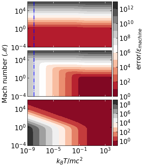
Figure 2 shows the contour plots of Equation 20 for the new scheme (top panel) and Equation 21 for the original scheme (middle panel) as a function of and temperature. The bottom panel shows the ratio of Equation 21 to Equation 20. It demonstrates the advantage of using . The top panel shows that using in the conversion scheme is almost error-free when dealing with subsonic flows at any finite temperature, including the low- limit. In supersonic flows, the numerical errors proportional to are common and caused by finite digits of floating numbers. In comparison, the middle panel shows the error using , which severely suffers from catastrophic cancellation in the low- limit even when . See also Figure 16 in Appendix B.
On the other hand, conversion from primitive to conserved variables is also needed in the Riemann solver. This procedure involves straightforward substitution without the need of root-finding. We use
| (22) |
and
| (23) |
to compute and , where can be computed from Equation 15 with known . Note that Equation 22 and Equation 23, following directly from Equation 10 and Equation 15 without any approximation, are written in a form without any subtraction to avoid catastrophic cancellation. In contrast, using Equation 5c and Equation 6 to compute the reduced energy density can suffer from catastrophic cancellation in the NR limit.
We close this section by providing a flowchart of the new conversion scheme in Figure 15 in Appendix B and by summarizing the equations actually solved by gamer-sr. Other mathematically equivalent forms are unrecommended as they may suffer from catastrophic cancellation in the UR or NR limit.
- •
- •
Lorentz factor: Equation 8.
- •
Four-velocities: Equation 17.
- •
Temperature: Equation 16.
- •
Pressure: Equation 18.
- •
Reduced enthalpy: Equation 22.
- •
Reduced energy density: Equation 23.
III Numerical Methods
III.1 A GAMER Primer
Due to the flexibility and extensibility of gamer (Schive et al. 2010; Schive et al. 2018), the SRHD module directly inherits the AMR structure and the MPI/OpenMP/GPU parallelization framework of hydrodynamics, and therefore we only provide a summary here. We define the base grid resolution as level-0 and the th refinement as level-, where level- has a spatial resolution times higher than that of the base level. Data in gamer are always decomposed into patches, each of which consists of cells, and the AMR implementation is realized by constructing a hierarchy of patches in an octree structure. According to user-defined refinement criteria, we can create or remove fine patches under the proper-nesting constraint.
In addition to the refinement criteria provided by the hydrodynamics module, we also implement two refinement criteria for SRHD: the gradient of the Lorentz factor and the magnitude of . The former aims to capture the thin and high- shell in the Sedov-Taylor blast wave, while the latter ensures that the spine region in an over-pressured jet (cf. Figure 13) can be fully resolved. For all refinement criteria, the refinement thresholds on different levels can be set independently as run-time parameters.
We port the routines involving massive floating-point operations to GPUs such as the SRHD solvers and time-step calculations. On the other hand, we use CPUs to perform ghost-zone interpolation and patch refinement. As a result, we recommend using the refinement criteria only involving conserved variable for better performance because conserved variables are readily available from memory. By contrast, primitive variables can only be obtained by root-finding iteration, which is computationally expensive.
For enhancing software portability and reusability, GAMER not only supports both CPU-only and GPU modes but also allows the same physics modules to be shared by both CPU and GPU computations. Specifically, in the CPU-only mode, we compute different grid patches in the same MPI process in parallel with OpenMP. In the GPU mode, we replace these OpenMP parallel clauses with CUDA thread blocks and then use threads within the same thread block to update all cells within the same grid patch. This scheme maximizes the reuse of physics routines, avoids redundant code development and maintenance, and significantly lowers the barrier of code extension, especially for developers not acquainted with GPU programming. We have utilized this CPU/GPU integration infrastructure in the SRHD implementation.
gamer-sr supports the MUSCL-Hancock (Toro 2011) and VL (Falle 1991; van Leer 2006) schemes for numerical integrations and a piece-wise linear method (PLM; van Leer 1979) for data reconstruction. For the Riemann solver, it supports both relativistic HLLC and HLLE solvers (Mignone & Bodo 2005; Mignone & Bodo 2006), which have been adapted not only to be compatible with the TM EoS by using the corresponding sound speed, Equation 14, but also to evolve the reduced energy density (i.e. replacing with ).
III.2 Flexible Time-step
gamer-sr provides two Courant-Friedrichs-Lewy (CFL) conditions for time-step determination. The first one is based on the local signal propagation speed, , which gives maximum allowed time-steps in a wide dynamical range. Thus, it can significantly improve performance when the maximum is not close to unity. The other is based on the speed of light, where we simply replace by . It gives the most conservative estimation of time-steps and is more time-consuming when the flow speed is far less than , although it is simple to implement and requires less computation.
To calculate , we first define to be a spatial unit vector in the direction of sound propagation, we then apply the Lorentz boost with velocity to the four-velocity of sound speed from local rest frame to laboratory frame. We finally obtain the four-velocity of signal that travels in laboratory frame as follows:
| (24) |
where and are the Lorentz factor of flow and of sound speed. is the four-velocity of sound speed defined by . Since the direction of the fastest signal propagation is in general parallel to flow velocity, we assume that both sound and flow propagate in the same direction (i.e. ). The spatial components of Equation 24 then reduce to
| (25) |
Motivated by Equation 25, we simply choose as the bound of each spatial component and sum over for each spatial component to obtain
| (26) |
where is the -component of the four-velocities of flow.
Note that Equation 26 is essentially the addition of flow speed and sound speed in special relativity theory. Converting Equation 26 back to three-velocity
| (27) |
and substituting Equation 27 into the CFL condition, we finally obtain the flexible time-step based on the local signal propagation speed for SRHD:
| (28) |
where is the cell spacing and the safety factor with a typical value of for MUSCL-Hancock and VL schemes.
III.3 Handling unphysical results
Unphysical results, for example, negative pressure, negative density and superluminal motion, can stem from the failure of the following criterion:
| (30) |
where the left-hand side involves the numerically updated quantities and is the machine epsilon – typically, for double precision and for single precision. The failure may take place in one of the following four steps:
(1) SRHD solver
SRHD solver is responsible for updating the conserved variables by a given time-step. If unphysical result occurs in a cell, we redo data reconstruction by reducing the original minmod coefficient by a factor of 0.75. If the failure still occurs, we further reduce the minmod coefficient repeatedly until Equation 30 passes or the reduced minmod coefficient vanishes. Note that interpolating with a vanished minmod coefficient is essentially equivalent to the piece-wise constant spatial reconstruction.
(2) Grid refinement
Unphysical results may occur during grid refinement when performing interpolations on parent patches. The remedy here is the same as that in the SRHD solver. We repeat the interpolation process with a reduced minmod coefficient on the conserved variables until Equation 30 passes or the minmod coefficient vanishes. A vanished minmod coefficient is essentially equivalent to directly copying data from the parent patch without interpolation.
(3) Ghost-zone interpolation
To preserve conservation, where the volume-weighted average of child patch data are equal to its parent patch data, we normally fill the ghost zones of the patches on level by interpolating the conserved variables on level when the ghost zones lie on level . However, if unphysical results occur, we interpolate primitive variables instead. Interpolating primitive variables is more robust than interpolating conserved variables since Equation 30 is always satisfied. After interpolation, we fill the ghost zones with the conserved variables derived from the interpolated primitive variables. Note that this procedure still preserves conservation because ghost zones do not affect conservation.
(4) Flux correction operation.
For a leaf coarse patch adjacent to a coarse-fine interface, the flux difference between the coarse and fine patches on the interface will be used to correct the coarse-patch conserved variables adjacent to this interface. If unphysical results are found after this flux correction, we simply ignore the correction on the failed cells. Skipping the correction will break the strict conservation but it only occurs rarely.
IV Test Problems
To understand how evolving the total energy density may deteriorate simulation results and to demonstrate how much the new scheme improves, we compare the results from evolving by the flux (original scheme) with that from evolving by the flux (new scheme). Since catastrophic cancellation is likely to occur in UR and NR limits, we will conduct several test problems in these two limits. All simulations throughout this paper adopt the HLLC Riemann solver and PLM data reconstruction unless otherwise specified.
IV.1 Convergence test for sinusoidal waves
We perturb proper mass density in the high- and low- limits to compare the accuracy of both schemes over a wide dynamical range. We construct the initial conditions as follows. All cases share homogeneous and static background with proper mass density on uniform grids, whereas the ambient temperatures are set to and for the high- and low- limits, respectively. We then sinusoidally perturb the background with a tiny amplitude, .
To monitor how errors in the numerical solution decrease as a function of increasing spatial resolution in the three-dimensional space, we adopt a propagating wave along the diagonal direction of the simulation cubic box with the periodic boundary condition. Thus, the analytical solution is , where is the sound speed given by Equation (14).
We define the L1-norm error as
| (31) |
where is the numerical solution of -th cell at and is the corresponding analytical solution. We then calculate the L1 error of the proper mass density along the wave propagating direction. As shown in Figure 3, the L1 errors of the new scheme in both the high- limit () and low- limit () decrease as , consistent with the second-order accuracy of the MUSCL-Hancock scheme with PLM data reconstruction. However, the error of the original scheme in the low- limit () is much larger and roughly equal to a constant of . This is expected because the error arising from the original scheme can be estimated from Equation 21 in the NR limit:
| (32) |
where and for double precision.
We thus conclude that for the original scheme in the NR limit, the cancellation between and leads to an error of when computing primitive variables, roughly consistent with the L1 error (). For the opposite high- limit (), the discretization error, however, completely overwhelms the error () estimated from Equation 21 in the high- limit, thus dominating the L1 error. The error arising from the cancellation in the new scheme, , on the left side of Equation 15, is close to in both the high- and low- limits when (see Section II.3 and Appendix B for details).
IV.2 1-D relativistic Riemann problems
The 1-D Riemann problem (Sod 1978) has played an important role by providing exact nonlinear solutions against which (relativistic) hydrodynamic codes can be tested. Riemann problem is an initial-value problem with a piece-wise constant initial data that has a single discontinuity in the domain of interest. In this subsection, we directly compare the new and original schemes by simulating two relativistic Riemann problems. We then demonstrate that the new scheme handles both the UR and NR limits very well. By contrast, the original scheme severely suffers from numerical errors in the NR limit. Both schemes share the same numerical setup, e.g., MUSCL-Hancock integration, PLM data reconstruction, hybrid van-Leer, generalized minmod slope limiter, and uniform grids with the outflow boundary condition. In addition, we have numerically derived the exact solution of a nontrivial relativistic Riemann problem with the TM EoS (see Appendix C for details) in order to verify the numerical results.
| Floating-point format | |||||||
|---|---|---|---|---|---|---|---|
| Ultra-relativistic limit | Double precision | ||||||
| Mixed limits | Single precision |
IV.2.1 Ultra-relativistic limit
We simulate a head-on collision of two identical gases with and with uniform 512 grids. The computational domain is in the interval . The initial discontinuity is located at . The first row of Table 1 presents the initial right and left states. Figure 4 shows the results at . The left panels show the entire simulation domain, while the right panels show the zoom-in image of the post-shock region, which has been violently heated up to ultra-relativistically hot temperature () by the extremely high- gases flowing inwards from both sides. As can be seen, the new scheme () fully agrees with the original scheme () on the large-scale profile but also on the small-scale errors, meaning that the new scheme does not sacrifice the numerical accuracy in the UR limit. In addition, we notice that the non-negligible and spurious waves occur in the post-shock region, which are not due to root-finding iterations but to spatial discretization errors as the spurious waves can be reduced by increasing spatial resolution.
IV.2.2 Mixed limits
To demonstrate that the new scheme can handle a large dynamical range covering both extremely hot and extremely cold gases, we simulate a nontrivial Riemann problem where the temperature straddles between the high- and low- limits. This initial condition evolves into a cold left-traveling rarefaction wave separated by a contact discontinuity to match an extremely hot downstream of an ultra-relativistic shock traveling toward the right. Also, we have numerically derived the exact solution of this particular Riemann problem with the TM EoS (see Appendix C). The second row in Table 1 shows the initial left and right states. The simulation adopts a computational domain [0,100] with 102,400 cells. Since the speed of the right-traveling shock is 276 times faster than that of the left-traveling rarefaction wave, we put the initial discontinuity at to provide an ample space for the right-traveling shock.
Figure 5 shows the results at , where there are three points to be emphasized. First, we find not only that the shock front at is well resolved by 3–4 cells but also that the new scheme () agrees well with the exact solution of the TM EoS (), as shown in all insets. Second, the L1 error, defined by Equation 31, of the density profile from the original scheme () is 23 per cent within the region between the head of rarefaction wave (, the third number from top in the leftmost column of Table 2 in Appendix C) and initial discontinuity (), consistent with the 20 per cent error estimated by Equation 32 with . Similar conclusions can be drawn for other physical quantities. However, in the region swept by the right-traveling contact discontinuity, errors of the original scheme are much larger than the estimate, which requires further investigation. Third, the solutions of the TM EoS () match well with both () in the NR region () and () in the UR region (). It demonstrates the capability of capturing the transition from (for ) to (for ) for the new scheme. The exact solutions of this test are shown in Table 2 in Appendix C.

.
IV.3 Multi-dimensional grid effects for high- flows
To investigate the detrimental impact of grid effects on the evolution of ultra-relativistic and high Mach number hydrodynamic problems, we separately simulate two identical three-dimensional mono-direction flow with different flow directions. One flow is along the diagonal direction of the simulation box and the other is parallel to the grid direction. Both simulations share the same numerical set-up as follows. Flows are initially represented by cylinders extending to the boundaries of a periodic cubic box with a width . The cylinder diameter is . The proper mass density ratio of the flow and the ambient is . The temperatures of the flows and the ambient are and , respectively. The four-velocity () profile inside the flow source is , where is the distance from the flow axis inside the source. Other physical quantities are uniformly distributed inside the source.
The AMR base level is covered by cells in all cases. We adopt the gradient of the proper mass density and the magnitude of as the two inclusive refinement criteria. We refine a patch if the gradient of a cell satisfies
| (33) |
where , , and is the cell size at refinement level . This criterion aims to capture the finger structure due to instabilities at the interface between the flow and the ambient gases. Also, a patch will be refined when any cell satisfies so that the high-speed region is refined to the finest level.
Figure 6 shows the simulation results at . In Figures 6 and 6, we adopt four AMR levels to ensure that the flow diameter can be resolved by 28 cells. The extremely high Mach number () flow leaves any instability short of time to develop, and one expects a smooth flow-ambient interface. However, the interface of the oblique flow turns out to be subject to severe dissipation. The fuzzy-looking cross-sections in the transverse slices of the oblique flow (right column in Figure 6) suggest that the dissipation is caused by numerical instabilities when high Mach number flow travels obliquely across Cartesian grids. This numerical problem is not limited to relativistic high Mach number flows but also occurs in non-relativistic high Mach number flows.
To examine this issue further, we increase the spatial resolution by a factor of 2 and decrease the time-step by a factor of 0.3 from the standard Courant condition. The results (Figures 6 and 6) indicate that increasing spatial and temporal resolution can neither significantly ameliorate the dissipation nor help the oblique flow converge to the horizontal flow. This artificial grid effect can adversely influence the study of high-speed jets, especially for hydrodynamical instabilities near the jet boundaries.
An example of this boundary instability is the finger-like pattern observed immediately outside the parallel flow (right column in Figure 6), which we believe to arise from a genuine instability seeded by discritization noise. The finger-like pattern has a higher temperature than the ambient, and in fact consists of two-dimensional flat sheets along the flow. This is demonstrated in Figure 7 with transverse slices cut through ‘B’ and ‘C’. The patterns are identical to that cut through ‘A’ in Figure 6. These 2-D sheet pattern persists even after adding 1 per cent level of white noise into the background density, illustrating that the coherence of sheets along the flow direction is genuinely generated by the high-speed flow boundaries. This finger pattern is similar, but not identical, to the curvature-driven fingers of a knotted jets reported recently (Gourgouliatos & Komissarov 2017). Our flow has a smooth and parallel boundary without any curvature to drive the fingers.


V Performance scaling
We measure both strong and weak scalings of gamer-sr with AMR and hybrid MPI/OpenMP/GPU parallelization. The simulations were conducted on the Piz-Daint supercomputer that provides a 12-core Intel Xeon E5-2690 CPU and a Tesla P100 GPU on each computing node. Strong and weak scalings are defined as how the simulation wall time varies with the number of computing nodes for a fixed total problem size and for a fixed problem size per node, respectively. We launch one MPI process with 12 OpenMP threads per node and enable GPU acceleration with single precision.
We divide this section into two parts. First, we measure the strong scaling of a relativistic jet simulation. The simulation set-up, such as initial condition, boundary condition, and grid refinement, follows those described in Section VI.2. Second, we present the weak scaling for periodic and spherical multi-blast waves test (see Figure 8).
(1) Strong scaling:
Figure 9 shows the strong scaling results. The parallel efficiency for strong scaling is defined by , where is the simulation wall time using nodes. is the number of nodes for reference and is fixed to 16 in our test. The overall performance reaches cell updates per second with 2048 GPU nodes, corresponding to a parallel efficiency of 45 per cent. The deviation from the ideal scaling is mainly due to MPI communication, the time fraction of which increases by a factor of 10 when increases from 64 to 2048.

(2) Weak scaling:
The periodic computational domain is composed of identical cubic subdomain, each of which has a volume of and has an explosion source at its own centre with a radius of and an ultra-relativistic temperature of . The uniform ambient gas has a non-relativistic temperature of and a density of . Each subdomain is composed of a base-level grid with three refinement levels, where we refine patches based on the gradient of the reduced energy density. All blast waves evolve from to . We measure the overall performance and parallel efficiency using nodes, where each node computes one subdomain. Figure 8 shows a temperature slice () through the centre of four blast waves at , with the grid patches overlaid.
Figure 10 shows the weak scaling results. The parallel efficiency for weak scaling is defined by , where is defined the same as the strong scaling. The parallel efficiency is measured to be 90 per cent with 64 nodes and 78 per cent with 2048 nodes, achieving a peak overall performance of cell updates per second with 2048 nodes. The drop of parallel efficiency is mainly due to MPI communication, the time fraction of which increases from 10.3 () to 18.8 per cent ().
We remark that the strong and weak scaling tests demonstrate 55 and 80 per cent parallel efficiencies, respectively, with 1024 nodes on the Piz-Daint supercomputer. Moreover, the peak performance on a single Tesla P100 GPU achieves cell updates per second, which is about one-third of the peak performance of non-relativistic hydrodynamics (Schive et al. 2018).
VI Astrophysical Applications
VI.1 Triaxial blast wave
This triaxial relativistic blast wave problem models a hypothetical astrophysical mega-explosion driven by an ultra-relativistically hot plasma source absent of particular symmetry. It is an atypical test for which we verify the code’s ability to deal with strong 3D shocks. The simulation evolves a blast wave from a triaxial source in a homogeneous medium. The triaxial source has aspect ratios with a semi-major axis aligned with the diagonal direction, where is the width of a cubic computational box. The source is filled with a uniform ultra-relativistic () plasma and the ambient is filled with a uniform non-relativistic () HII gas. The density is homogeneous throughout the entire domain with . After the system quickly relaxes, the hot plasma rapidly expands driving a forward shock traveling almost at the speed of light.
The AMR base level is covered by cells with the periodic boundary condition. The highest refinement level is 9 so that the initial source can be adequately resolved by approximately 82 cells along the minor axis. To refine both the initial source and the thin shell of the blast wave shock, we adopt the gradient of the reduced energy density as the refinement criterion, with and in Equation 33.
For comparison, we also simulate a spherical blast wave to understand how the initially triaxial shape affects the evolution of the ultra-relativistic blast wave. Both the spherical and triaxial cases have the same simulation set-up and the same source volume, i.e. , where is the radius of the spherical source.
Figure 11 shows the results. We observe that the interior hot plasma pushes out a contact discontinuity immediately inward of the shock and that the thickness of the shell between the contact discontinuity and the shock diminishes in time. In early time, the triaxial profiles () at deviate from the spherical counterparts (), especially in the pressure and proper mass density, although the shock positions almost coincide. However, at a later time, the profiles at show no significant difference between the triaxial () and spherical () blast waves, indicating the initial shape of the source does not have a great impact on the asymptotic evolution of ultra-relativistic blast waves.
To further investigate how the triaxial blast wave evolves into a spherical one, we extract the radii and of the triaxial blast wave along the semi-major () and semi-minor axes () of the initial source from simulation data. As shown in Figure 12, we find that the dimensionless quantity is approximately equal to . This dependence suggests that the triaxiality is damped out with the blast wave propagation by the relation:
| (34) | ||||
We remark that this test problem also demonstrates that gamer-sr can successfully handle ultra-relativistic gases embedded in a cold HII region, which can be difficult for conventional SRHD codes.

VI.2 Limb-brightened jet
Most active galactic nuclei (AGN) jets in VLBI observations appear ridge-brightened, while limb-brightened jets are rare and have been reported only in a few nearby radio galaxies, such as Mrk 501 (Giroletti et al. 2004), M87 (Asada & Nakamura 2012; Kim et al. 2018), Cygnus A (Boccardi et al. 2015), and 3C84 (Nagai et al. 2014; Giovannini et al. 2018). Motivated by these observations, we simulate a three-dimensional SRHD jet using gamer-sr to study its acceleration and collimation in the hope to shed light on the limb-brightened jets.
We adopt the gradient of the reduced energy density and the magnitude of as the two inclusive refinement criteria. A patch is refined if any cell satisfies either Equation 33 with and or . The first criterion aims to capture the strong terminal shock and the cocoon, while the second one ensures that the central ‘spine’ region of the jet can be properly resolved.
The jet is continuously ejected from a cylindrical source with four-velocity (). The proper mass density ratio between the jet source and the ambient gases is set to 1.0. The temperature () of the source and the ambient gases are set to 0.5 and , respectively. The outflow is thus an extremely under-pressured jet. Both the diameter and the length of the cylindrical source are well resolved by 32 cells.
Figure 13 shows the simulation results. It demonstrates that the jet flow is entirely confined by a turbulent cocoon at all time. Two points are worth noting from these longitudinal slices. First, the Lorentz factor (first row) rises from to , and meanwhile the temperature (second row) drops from 0.5 to 0.01 along the jet. Second, the relativistic Bernoulli number minus (fifth row), defined as , remains nearly constant within the spine region. According to the de Laval nozzle effect, these suggest that thermal energy is converted to kinetic energy by the expansion of a supersonic flow. Surprisingly, the gases are still accelerated in the region between the label ‘C’ and the confinement point close to ‘D’. These images seem to suggest acceleration during flow convergence, which in fact does not contradict the de Laval nozzle effect. The gases still expands away from the jet axis after passing ‘C’, which can be confirmed by examining the transverse slice of the radial component of the Mach number (the last row),
| (35) |
where is the cylindrical unit radial vector, is the four-velocity of flow, and . The definition of the radial Mach number given by Equation 35 is Lorentz invariant when the transforming direction is along the jet. Obviously, gases expand not only between the jet source and ‘C’, but also inside the entire central spine region. Thus, the flow convergence in between ‘C’ and ‘D’ is a false impression.
Associated with this expanding jet flow is the limb-brightened phenomenon. Confined by the cocoon, the radial flow of the cooler jet imparts onto the cocoon with a boundary shock, as signified by the edge . Hot gases in the post-shock region then diffuse into the cocoon transverse to the jet through some instabilities composed of high-density and low-temperature fingers. This finger pattern is similar to that reported in Section IV.3.
Certainly the boundary shock can generate particle acceleration and produce extra synchrotron brightness at the jet edge, thus yielding limb brightening. Since the boundary shock is relatively weak, the extra synchrotron brightness cannot be immense. This may explain why limb brightening is mostly observed in nearby AGN jets.

VII conclusions
In this paper, we have presented a novel special relativistic hydrodynamics code, gamer-sr, which incorporates a new, well-tailored conversion scheme (cf. Figure 15) between primitive and conserved variables, together with the Taub-Mathews equation of state (TM EoS) covering both the ultra-relativistic and non-relativistic limits. The new scheme adopts the four-velocity , the reduced energy density , and the reduced enthalpy to effectively avoid the catastrophic cancellation in subsonic flows at all finite temperature, including the particularly challenging low-temperature regime, with errors decreasing as when .
We have numerically derived the exact solution of a Riemann problem covering both extreme cold and ultra-relativistically hot gases with the TM EoS. Simulation results using our new scheme are in very good agreement with the exact solution in both the ultra-relativistic and non-relativistic regimes. (cf. Figure 5). In comparison, the catastrophic cancellation arising from the original (unoptimized) scheme can be much more severe than the truncation error in the non-relativistic limit, especially in the region swept by a traveling contact discontinuity.
The new scheme has been integrated into the code gamer to facilitate the hybrid OpenMP/MPI/GPU parallelization and adaptive mesh refinement. Thanks to that, the performance of the root-finding iterations in the TM EoS can be significantly improved by GPU. The parallel efficiency using 2048 computing nodes is measured to be 45 per cent for strong scaling (cf. Figure 9) and 75 per cent for weak scaling (cf. Figure 10) on the Piz-Daint supercomputer.
gamer-sr has been demonstrated to be able to handle ultra-relativistic flow with a Lorentz factor as high as . However, we also find that the Cartesian grids can lead to artificial dissipation when the direction of a high Mach number flow is not aligned with grids. This problem cannot be mitigated by increasing spatial and temporal resolution.
We have examined two astrophysical problems with coexisting relativistically hot and cold gases to demonstrate the power of gamer-sr. The first problem deals with a relativistic blast wave with a triaxial source. Not only do we find that the code is able to capture the ultra-relativistic strong shock very well, but we also discover a simple rule governing how the triaxiality of the blast wave diminishes as a function of the blast wave radius.
The second problem addresses the flow acceleration and limb-brightening of a relativistic AGN jet. We find that the jet, from its head to its source, is always enclosed inside a turbulent cocoon. The jet is accelerated all the way up to the first confinement point, where an internal shock appears. We attribute such flow acceleration to the relativistic Bernoulli’s law. In addition, the synchrotron limb-brightening is found to be caused by the jet transverse boundary shock, outside which the post-shock cosmic-ray particles are mixed with the turbulent cocoon and give out extra synchrotron emission.
Acknowledgement
P.T. thanks Kuo-Chuan Pan for helping conduct the parallel scaling tests at CSCS (Piz-Daint) under Grant No. 661. H.S. acknowledges funding support from the Jade Mountain Young Scholar Award No. NTU-109V0201, sponsored by the Ministry of Education, Taiwan. This research is partially supported by the Ministry of Science and Technology (MOST) of Taiwan under Grants No. MOST 107-2119-M-002-036-MY3 and No. MOST 108-2112-M-002-023-MY3, and the NTU Core Consortium project under Grants No. NTU-CC-108L893401 and No. NTU-CC-108L893402.
Data Availability
The data underlying this article are available in the article and in its online supplementary material.
References
- Asada & Nakamura (2012) Asada K., Nakamura M., 2012, The Astrophysical Journal, 745, L28
- Blandford et al. (2019) Blandford R., Meier D., Readhead A., 2019, Annual Review of Astronomy and Astrophysics, 57, 467
- Boccardi et al. (2015) Boccardi B., Krichbaum T. P., Bach U., Mertens F., Ros E., Alef W., Zensus J. A., 2015, A and A, 585, A33
- Chiueh (1989) Chiueh T., 1989, Phys. Rev. Lett., 63, 113
- Chiueh et al. (1991) Chiueh T., Li Z.-Y., Begelman M. C., 1991, ApJ, 377, 462
- Chiueh et al. (1998) Chiueh T., Li Z.-Y., Begelman M. C., 1998, The Astrophysical Journal, 505, 835
- Falle (1991) Falle S. A. E. G., 1991, Monthly Notices of the Royal Astronomical Society, 250, 581
- Fong et al. (2019) Fong W., et al., 2019, ApJ, 883, L1
- Fryxell et al. (2000) Fryxell B., et al., 2000, The Astrophysical Journal Supplement Series, 131, 273
- Ghirlanda et al. (2019) Ghirlanda G., et al., 2019, Science, 363, 968
- Giovannini et al. (2018) Giovannini G., et al., 2018, Nature Astronomy, 2, 472
- Giroletti et al. (2004) Giroletti M., et al., 2004, The Astrophysical Journal, 600, 127
- Gourgouliatos & Komissarov (2017) Gourgouliatos K. N., Komissarov S. S., 2017, Nature Astronomy, 2, 167
- Higham (2002) Higham N. J., 2002, Accuracy and Stability of Numerical Algorithms, 2nd edn. Society for Industrial and Applied Mathematics, USA
- Jüttner (1911) Jüttner F., 1911, Annalen der Physik, 339, 856
- Kennel & Coroniti (1984a) Kennel C. F., Coroniti F. V., 1984a, ApJ, 283, 694
- Kennel & Coroniti (1984b) Kennel C. F., Coroniti F. V., 1984b, ApJ, 283, 710
- Kim et al. (2018) Kim J.-Y., et al., 2018, A&A, 616
- Li et al. (1992) Li Z.-Y., Chiueh T., Begelman M. C., 1992, ApJ, 394, 459
- Lora-Clavijo et al. (2015) Lora-Clavijo F. D., Cruz-Osorio A., Guzmán F. S., 2015, The Astrophysical Journal Supplement Series, 218, 24
- Martí & Müller (1994) Martí J. M., Müller E., 1994, Journal of Fluid Mechanics, 258, 317
- Mathews (1971) Mathews W. G., 1971, ApJ, 165, 147
- Mignone & Bodo (2005) Mignone A., Bodo G., 2005, Monthly Notices of the Royal Astronomical Society, 364, 126
- Mignone & Bodo (2006) Mignone A., Bodo G., 2006, Monthly Notices of the Royal Astronomical Society, 368, 1040
- Mignone & McKinney (2007) Mignone A., McKinney J. C., 2007, Monthly Notices of the Royal Astronomical Society, 378, 1118
- Mignone et al. (2005) Mignone A., Plewa T., Bodo G., 2005, The Astrophysical Journal Supplement Series, 160
- Mooley et al. (2018a) Mooley K. P., et al., 2018a, Nature, 554, 207
- Mooley et al. (2018b) Mooley K. P., et al., 2018b, Nature, 561, 355
- Nagai et al. (2014) Nagai H., et al., 2014, The Astrophysical Journal, 785, 53
- Noble et al. (2006) Noble S. C., Gammie C. F., McKinney J. C., Zanna L. D., 2006, The Astrophysical Journal, 641, 626
- Núñez-de la Rosa & Munz (2016) Núñez-de la Rosa J., Munz C.-D., 2016, MNRAS, 460, 535
- Rezzolla & Zanotti (2018) Rezzolla L., Zanotti O., 2018, Relativistic hydrodynamics. Oxford University Press
- Rezzolla et al. (2001) Rezzolla L., Zanotti O., Pons J. A., 2001, Journal of Fluid Mechanics, 449, 395
- Ryu et al. (2006) Ryu D., Chattopadhyay I., Choi E., 2006, The Astrophysical Journal Supplement Series, 166, 410
- Schive et al. (2010) Schive H.-Y., Tsai Y.-C., Chiueh T., 2010, The Astrophysical Journal Supplement Series, 186, 457
- Schive et al. (2018) Schive H.-Y., ZuHone J. A., Goldbaum N. J., Turk M. J., Gaspari M., Cheng C.-Y., 2018, Monthly Notices of the Royal Astronomical Society, 481, 4815
- Sod (1978) Sod G. A., 1978, Journal of Computational Physics, 27, 1
- Synge (1957) Synge J. L., 1957, North-Holland Pub. Co.; Interscience Publishers
- Taub (1948) Taub A. H., 1948, Physical Review, 74, 328
- Toro (2011) Toro E. F., 2011, Riemann solvers and numerical methods for fluid dynamics : a practical introduction. Springer, Berlin
- Turk et al. (2011) Turk M. J., Smith B. D., Oishi J. S., Skory S., Skillman S. W., Abel T., Norman M. L., 2011, The Astrophysical Journal Supplement Series, 192, 9
- Woosley (1993) Woosley S. E., 1993, ApJ, 405, 273
- van Leer (1979) van Leer B., 1979, Journal of Computational Physics, 32, 101
- van Leer (2006) van Leer B., 2006, pp 192–206
Note that the speed of light, the particle mass, and the Boltzmann constant are set to unity in Appendix for simplicity.
Appendix A Initial guess for Newton-Raphson iteration
We use the Newton-Raphson iteration to find the root of Equation (15). The iteration requires the derivative of Equation 15 with respect to :
| (A1) |
where
| (A2) |
follows from Equation 16.
The root-finding iteration also requires an initial guess of , for which we suggest the following procedure. In the low- limit, we Taylor expand Equation (15) in powers of and keep the first- and second-order terms:
| (A3) |
Solving Equation (A3) for the unknown gives the positive solution:
| (A4) |
In the opposite high- limit, Equation (15) can be reduced to
| (A5) |
which leads to
| (A6) |
Equation (A4) and Equation (A6) provide two initial guesses for ‘cold’ and ‘hot’ gases, respectively. The threshold to distinguish between ‘cold’ gases and ‘hot’ gases is given by
| (A7) |
which is obtained by equating Equations (A4) and (A6) (see Figure 14). If is greater than Equation A7, we choose Equation (A6) as an initial guess for the Newton-Raphson iteration (hot gases); otherwise, we choose Equation A4 (cold gases).

Appendix B Numerical error analysis for root-finding
Figure 15 provides a detailed flowchart of the conversion between primitive and conserved variables. Figure 16 demonstrates that the numerical errors of root-finding arising from the new and original conversion schemes are consistent with the predicted values given by Equation 20 and Equation 21. We measure this conversion error by first converting the input primitive variables into conserved variables . Next, we convert back to and then measure the relative error between and . Since the catastrophic cancellation is more prominent in the low- limit, we measure the error as a function of Mach number from to with a fixed non-relativistic temperature (i.e. the blue dashed-dotted line in Figure 2). To verify the accuracy in three-dimensional space, we choose the direction of four-velocity to be parallel to the line (i.e. for all ). Double precision is adopted to handle the large dynamic range. Figure 16 confirms that the numerical errors of the new and original schemes are mainly caused by round-off errors in the calculation of and , respectively.
Appendix C Exact solutions of relativistic Riemann problems with the TM equation of state
To derive the exact solutions of relativistic Riemann problems with the TM EoS, we have generalized the previous framework of a constant polytropic EoS (Martí & Müller 1994; Rezzolla et al. 2001) to the TM EoS. More precisely, this approach can be applied to any EoS once we know the relationship between enthalpy and temperature. Here we only summarize the important equations and highlight salient differences from the polytropic EoS. We use the subscripts to refer to the left/left-contact/right-contact/right regions and define the relative four-velocity of with respect to as . Note that we have replaced three-velocity with four-velocity again to avoid catastrophic cancellation in the ultra-relativistic limit.
The exact solution of a relativistic Riemann problem with the TM EoS can be obtained through the following three steps:
- 1.
For a given initial condition, we can determine the wave pattern by comparing the relative velocity between the two unperturbed initial states with the three limiting values. These values mark the transition from one wave pattern to another and can be directly computed from the initial condition. See Rezzolla et al. 2001 for details.
- 2.
We determine the unknown pressure between the left and right waves by numerically solving
(C1) where , , and . Note that the four-velocity in the left-/right-contact region, , is different for each of the three possible wave patterns. For example, if the left wave is rarefaction and the right wave is shock, then and where and are defined as follows.
- (a)
represents the relation between pressure and flow four-velocity behind the rarefaction wave:
Given the pressure behind the rarefaction wave (i.e. ) during the Newton-Raphson iteration for solving Equation C1, we can determine by numerically solving the system of equations (10), (14), (18), (C2a), and (C2b):(C2a) (C2b) Hereafter, the upper/lower sign applies to the right/left wave. The ordinary differential equation (C2a), known as the Riemann invariant (Rezzolla & Zanotti 2018), relates the dynamical () and thermal () quantities. Equation C2b, derived from Equation 10 and the second law of thermodynamics, results from the fact that entropy is constant through the rarefaction wave. The ‘constant’ in Equation C2b is a function of entropy and can be determined by the thermal quantities in the region unperturbed by the rarefaction wave. In the case of the constant polytropic EoS, Equation C2b reduces to a familiar form: .
- (b)
represents the relation between pressure and flow four-velocity behind the shock wave:
Let ‘up/down’ denote the upstream/downstream state of the shock wave. Under the condition that ( in this case) is given during the Newton-Raphson iteration for solving Equation C1, we can compute by numerically solving the jump condition of the enthalpy:(C3) Equation C3 is known as the Taub adiabat (Taub 1948), where can be eliminated using Equations (16) and (18). After determining by a root-finding routine, the mass flux across the shock can be calculated by
(C4) The four-velocities of shock and post-shock then follow from
(C5) and
(C6) respectively. Equations (C5) and (C6) are essentially the Lorentz boost that takes four-velocity from the shock rest frame to the lab frame. Note that the mass flux is an invariant under the Lorentz boost in the flow direction.
- (a)
- 3.
Once is known, follows from Equations (16) and (18), which in turn allows for computing and through Equation C5 and Equation C6. On the other hand, behind the rarefaction wave follows from solving the system of equations (10), (18), and (C2b). Finally, given the self-similar and isentropic character of the rarefaction wave, and within the rarefaction fan can be computed by solving the system of equations (C2a) and , where .
Based on the above procedure, we show in Table 2 the exact solution of the relativistic Riemann problem given in the last row of Table 1 with the TM EoS at . The source code is available at (https://github.com/zengbs/ExactSolutionRelativisticRiemannProblem).
| 0.0000000000000000e+00 | 1.0000000000000000e+02 | +1.0000000000000000e-03 | 1.0000000000000000e-04 |
| 2.5743971630613077e-02 | 1.0000000000000000e+02 | +1.0000000000000000e-03 | 1.0000000000000000e-04 |
| 2.6720534130613077e-02 | 9.9999999999999986e+01 | +1.0000000000000002e-03 | 1.0000000000000000e-04 |
| 2.8673659130613080e-02 | 9.8588362795909134e+01 | +1.0183105709873300e-03 | 9.7658360819209613e-05 |
| 3.1603346630613080e-02 | 9.6495914226915929e+01 | +1.0457764274335814e-03 | 9.4228343648087098e-05 |
| 3.6486159130613087e-02 | 9.3074657510006034e+01 | +1.0915528549894106e-03 | 8.8726314406083176e-05 |
| 4.2345534130613087e-02 | 8.9077088828567909e+01 | +1.1464845688462534e-03 | 8.2466343818876140e-05 |
| 5.2111159130613087e-02 | 8.2671707042031258e+01 | +1.2380374291888151e-03 | 7.2821829638494934e-05 |
| 6.4806471630613094e-02 | 7.4813960019366874e+01 | +1.3570561601099081e-03 | 6.1655409508574801e-05 |
| 8.4337721630613108e-02 | 6.3723430244968533e+01 | +1.5401619444173906e-03 | 4.7188055213551995e-05 |
| 1.1168147163061304e-01 | 5.0121316453652021e+01 | +1.7965101817141935e-03 | 3.1625521037347636e-05 |
| 1.5172053413061287e-01 | 3.3922515604881056e+01 | +2.1718776864619303e-03 | 1.6499866085321606e-05 |
| 2.0836115913061276e-01 | 1.7591444669719621e+01 | +2.7028867092515813e-03 | 5.5229310921865207e-06 |
| 2.0933772163061276e-01 | 1.7369735883307754e+01 | +2.7120420544404751e-03 | 5.4074080094554571e-06 |
| 2.0972078270771960e-01 | 1.7283280852025452e+01 | +2.7156332803617649e-03 | 5.3626249948767070e-06 |
| 2.6627329885804002e-01 | 1.7283280852025452e+01 | +2.7156332803617649e-03 | 5.3626249948767070e-06 |
| 2.6724986145813656e-01 | 4.0108528993879889e-10 | +2.7156332816129858e-03 | 5.3626249948767070e-06 |
| 2.6909288248391281e+01 | 4.0108528993879889e-10 | +2.7156332816129858e-03 | 5.3626249948767070e-06 |
| 2.6910264810891281e+01 | 9.9999999999999998e-13 | -1.0000000000000000e+02 | 1.0000000000000000e-10 |
| 1.0000000000000000e+02 | 9.9999999999999998e-13 | -1.0000000000000000e+02 | 1.0000000000000000e-10 |