Bayesian Conditional Transformation ModelsThanks: Nadja Klein gratefully acknowledges funding from the DFG through the Emmy Noether grant
   KL 3037/1-1. The authors would like to thank the Editor, Associate Editor and two referees for
   many valuable comments that lead to a significant improvement of our original submission.
   nadja.klein@hu-berlin.de

Let $\text{\boldmath$a$}_{j}(y)$ and $\text{\boldmath$b$}_{j}(\text{\boldmath$x$})$ denote vectors containing basis function evaluations $B_{j1d_{1}}(y),d_{1}=1,\ldots D_{1}$ and $B_{j2d_{2}}(\text{\boldmath$x$}),d_{2}=1,\ldots,D_{2}$ for the response and the covariates, respectively, such that $\text{\boldmath$a$}_{j}(y)^{\top}=(B_{j11}(y),\ldots,B_{j1D_{1}}(y))$, and $\text{\boldmath$b$}_{j}(\text{\boldmath$x$})^{\top}=(B_{j21}(y),\ldots,B_{j2D_{2}}(y))$. Denoting by $\otimes$ the usual Kronecker product, we then obtain the most general form of partial transformation function in a BCTM as $\text{\boldmath$c$}_{j}(y,\text{\boldmath$x$})^{\top}=(\text{\boldmath$a$}_{j}(y)^{\top}\otimes\text{\boldmath$b$}_{j}(\text{\boldmath$x$})^{\top})^{\top}$, leading to

Essentially, the Kronecker product establishes a parametric interaction by forming pairwise products of the basis functions $B_{j1d_{1}}(y)$ and $B_{j2d_{2}}(\text{\boldmath$x$})$. The derivative with respect to $y$ is therefore also a tensor product involving the differentiated basis functions $B^{\prime}_{j1d_{1}}(y)=\partial B_{j1d_{1}}(y)/\partial y$. Specific restrictions on the two components of the tensor product lead to interesting special cases of the partial transformation function:

• •

  Setting $\text{\boldmath$a$}_{j}(y)\equiv 1$ leads to simple shift effects that only depend on the covariates.

• •

  Setting $\text{\boldmath$b$}_{j}(\text{\boldmath$x$})\equiv 1$ yields an effect of only $y$ that induces changes of the distributional shape (up to other effects).

• •

  Linear effects $\text{\boldmath$a$}_{j}(y)=(1,y)$ induce varying coefficient type effects where covariate effects linearly interact with the responses and the response takes the role of the interaction variable while the covariates are the effect modifiers.

Restricting our generic model to

leads to a location-shift transformation model that comprises various earlier transformation models as special cases. In this case, only the location of the transformed response depends on the covariates via $h_{\text{\boldmath$x$}}(\text{\boldmath$x$})$ and higher moments are captured unconditionally by the monotonic transformation $h_{Y}(y)$. This model type is parametrized by restricting the joint basis to $\text{\boldmath$c$}(y,\text{\boldmath$x$})^{\top}=((\text{\boldmath$a$}(y)^{\top}\otimes 1)^{\top},(1\otimes\text{\boldmath$b$}(\text{\boldmath$x$})^{\top})^{\top})=(\text{\boldmath$a$}(y)^{\top},\text{\boldmath$b$}(\text{\boldmath$x$})^{\top})^{\top}$ resulting in the shift transformation model $\text{\boldmath$c$}(y,\text{\boldmath$x$})^{\top}\text{\boldmath$\gamma$}=\text{\boldmath$a$}(y)^{\top}\text{\boldmath$\gamma$}_{1}+\text{\boldmath$b$}(\text{\boldmath$x$})^{\top}\text{\boldmath$\gamma$}_{2}$.

We are relying on B-splines for the response dimension while various alternatives are available for the covariate dimension (see Sec. 2.3 for details). The choice of B-splines for representing $\text{\boldmath$a$}_{j}(y)$ is mainly determined by the availability of suitable reparameterisations of the corresponding basis coefficients that ensure monotonicity along $y$ in the tensor product for the partial response transformations and well-studied smoothness properties. More precisely, we follow Pya and Wood 2015 and reparameterize the $D=D_{1}D_{2}$ dimensional basis vector $\text{\boldmath$\gamma$}_{j}=(\gamma_{j11},\ldots,\gamma_{j1D_{2}},\gamma_{j21},\ldots,\gamma_{jD_{1}D_{2}})^{\top}$ in two steps. First, we set $\text{\boldmath$\gamma$}_{j}=\mathbf{\Sigma}_{j}\text{\boldmath$\tilde{\beta}$}_{j}$, where $\mathbf{\Sigma}_{j}=\mathbf{\Sigma}_{D_{1}}\otimes\text{\boldmath$I$}_{D_{2}}$, $\text{\boldmath$I$}_{D_{2}}$ is an identity matrix of size $D_{2}$, $\mathbf{\Sigma}_{D_{1}}$ is a lower triangular matrix of size $D_{1}$ with $\Sigma_{D_{1},kl}=0$ if $k<l$ and $\Sigma_{D_{1},kl}=1$ if $k\geq l$, and the vector $\text{\boldmath$\tilde{\beta}$}_{j}$ is

Starting with a vector $\text{\boldmath$\beta$}_{j}=(\beta_{j11},\ldots,\beta_{j1D_{2}},\beta_{j21},\ldots\beta_{j2D_{2}},\ldots,\beta_{D_{1}1},\ldots,\beta_{jD_{1}D_{2}})^{\top}\in\mathbb{R}^{D}$ of unconstrained parameters, these choices ensure that the vector of basis coefficients $\text{\boldmath$\gamma$}_{j}$ is strictly increasing along the response dimension $y$ which, in turn, implies a tensor product effect that is monotonically increasing along $y$. The complete model vectors of basis coefficients are then given by $\text{\boldmath$\beta$}=(\text{\boldmath$\beta$}_{1}^{\top},\ldots,\text{\boldmath$\beta$}_{J}^{\top})^{\top}$ and $\text{\boldmath$\tilde{\beta}$}=(\text{\boldmath$\tilde{\beta}$}_{1}^{\top},\ldots,\text{\boldmath$\tilde{\beta}$}_{J}^{\top})^{\top}$, while the overall model matrix $\mathbf{\Sigma}$ is block diagonal with $\mathbf{\Sigma}_{1},\ldots,\mathbf{\Sigma}_{J}$ as diagonal elements. We formalize the monotonicity of $h(y|\text{\boldmath$x$})$ along the $y$ dimension in the following theorem.

In contrast to the MLT model introduced by Hothorn et al. 2018 that uses Bernstein polynomials as a basis for nonlinear effects, the BCTM is supplemented with a smoothness-inducing penalty through its prior and is therefore in principle less restrained regarding the number of model terms $J$ and functional complexity in direction of the covariates.

Of course, other basis function representations than B-splines are immediately conceivable for $\text{\boldmath$a$}_{j}(y)$. The main requirements for a suitable specification include the ability to incorporate monotonicity constraints, the analytical availability of the basis functions and their derivatives, and the numerically stable evaluation of these. While B-splines fulfill these requirements, investigating other choices and their properties is a promising avenue for future research.

Overfitting of unregularized splines can be avoided in our Bayesian framework by enforcing smoothness and regularization through shrinkage priors. For the special case of B-splines, Bayesian P-splines assign multivariate Gaussian priors to the regression coefficient vectors. We follow Kneib et al. 2019 and adopt this principle to tensor product terms such that the prior for the coefficient vector $\text{\boldmath$\beta$}_{j}$ associated with one of the partial transformation functions $h_{j}$ in (4) is multivariate Gaussian with expectation zero and precision matrix

where $\text{\boldmath$K$}_{j1}$ and $\text{\boldmath$K$}_{j2}$ are potentially rank deficient prior precision matrices of dimensions ($D_{1}\times D_{1}$) and ($D_{2}\times D_{2}$), respectively, controlling the type of smoothness required along the response and the covariate dimension, respectively. For the response dimension, we set $\text{\boldmath$K$}_{1j}=\text{\boldmath$D$}_{1j}^{\top}\text{\boldmath$D$}_{1j}$ where $\text{\boldmath$D$}_{1j}$ is a $(D_{1}-2)\times D_{1}$ partial first difference matrix consisting only of zeros except that $\text{\boldmath$D$}_{j}[d_{1},d_{1}+1]=-\text{\boldmath$D$}_{j}[d_{1},d_{1}+2]=1$ for $d_{1}=1,\ldots,D_{1}-2$ (Pya and Wood 2015; Pya 2010). The prior precision matrix $\text{\boldmath$K$}_{2j}$ shrinks in the direction of the respective covariate and the specific choice depends on the considered covariate effect of interect (see Sec. 2.3 for some examples). For monotonic nonlinear effects, the resulting penalty is quadratic in the (non-exponentiated) parameters $\text{\boldmath$\beta$}_{j}$. This corresponds to log differences in $\gamma_{jd_{1}d_{2}}$ for $d_{1}>2$, such that a first order random walk prior penalizes the squared differences between adjacent $\beta_{jd_{1}d_{2}}$, resulting in shrinkage towards a straight line, similar to second order random walk penalties for univariate P-splines (Pya and Wood 2015). The complete prior precision matrix $\text{\boldmath$K$}\equiv\text{\boldmath$K$}(\text{\boldmath$\tau$}^{2},\text{\boldmath$\omega$})$ is given as the block diagonal matrix with matrices $\text{\boldmath$K$}_{j}$ as diagonal elements. We formalize the prior for $\text{\boldmath$\gamma$}_{j}$ in the following proposition.

The amount of smoothness induced by the precision matrix (7) is controlled by the overall smoothing variance $\tau_{j}^{2}>0$ and the weight parameter $\omega_{j}\in[0,1]$. Following Kneib et al. 2019, we assume a discrete prior for the latter which has the advantage that generalized determinants of $\text{\boldmath$K$}_{j}$ can be pre-computed which considerably facilitates the numerically efficient implementation while still enabling anisotropic amounts of smoothness along the response and the covariate dimension. A uniform prior on a moderate number of equi-spaced values is used as a default for $\omega_{j}$. For the smoothing variance $\tau_{j}^{2}$, we consider two alternatives: Standard inverse gamma (IG) priors $\tau_{j}^{2}\sim\mathrm{IG}(a_{j},b_{j})$ where the hyperparameters are chosen among popular combinations such as $a_{j}=1$, $b_{j}=0.001$ to mimic a weakly informative setting, and scale-dependent (SD) hyperpriors as suggested in Klein and Kneib 2016. The latter results in a Weibull prior for $\tau_{j}^{2}$ with shape parameter $0.5$ and scale parameter $\theta$ determined from a scaling criterion on expected effect sizes. We transfer this concept to partially monotonic tensor product effects where, to achieve numerical stability, it is important to control the variation of those parameters exponentiated in (6). More precisely, we consider the scaling criterion $\mathbb{P}\left(\max_{d_{1}=2,\ldots,D_{1},d_{2}=1,\ldots,D_{2}}|\beta_{jd_{1},d_{2}}|\leq c\right)=1-\alpha$ with user-specified values for $c$ and $\alpha$. To determine the marginal prior distribution of $\tau_{j}^{2}$ required to evaluate the scaling criterion, we follow a simulation-based approach to marginalize out any additional hyperparameters. From the support of the exponential function, $c=3$ and $\alpha=0.01$ are useful standards also used later in our empirical studies.

In a last step, we collect all model parameters in the vector

with joint prior $\pi_{\text{\boldmath$\vartheta$}}(\text{\boldmath$\vartheta$})$ which can be factorized into products of the individual priors. The coefficient $\beta_{0}$ denotes the intercept of the model, while $\beta$, $\text{\boldmath$\tau$}^{2}$, $\omega$ are used to denote all basis coefficients, smoothing variances and anisotropy weights, respectively.

We highlight special cases of bases $\text{\boldmath$b$}(\text{\boldmath$x$})$ relevant for our applications:

• •

  Linear effects. The basis for linear effects of covariates $x_{1},\ldots,x_{p}$ collected in $x$ is $\text{\boldmath$b$}_{j}(\text{\boldmath$x$})^{\top}=(x_{1},\ldots,x_{p})^{\top}$ and we use a non-informative prior with $\text{\boldmath$K$}_{2j}=\bm{0}$. This also applies to the overall intercept $\beta_{0}$ when centering the partial transformation functions.

• •

  Random effects. Random effects (or frailties) are based on a grouping indicator $g\in\{1,\ldots,G\}$. The resulting $G$-dimensional basis vector $\text{\boldmath$b$}_{j}(g)$ has entry one if $y$ belongs to group $g$ and zero otherwise and we set $\text{\boldmath$K$}_{2j}=\text{\boldmath$I$}_{G}$ for i.i.d. random effects.

• •

  Discrete spatial effects. Similar to random effects, a spatial effect of a discrete spatial variable $s\in\{1,\ldots,S\}$ is constructed as an indicator with entries in the $S$-dimensional basis vector $\text{\boldmath$b$}_{j}(s)$ set to one if $y$ belongs to region $s$ and zero otherwise. We induce spatial smoothing in form of a Gaussian Markov random field (Rue and Held 2005, GMRF) prior. The precision matrix $\text{\boldmath$K$}_{2j}$ reflects the spatial orientation of the data, i.e. we define two regions as neighbours if they share a common border.

For an overview on possible bases for discrete (count) responses we refer the reader to Carlan and Kneib 2022.

As already stated, it is the task of the conditional transformation function $h(y|\text{\boldmath$x$})$ to transform the response values conditionally on the explanatory variables $x$ such that they follow the reference distribution $F_{Z}$. In that light, $F_{Z}$ plays a similar role as the inverse known link function in prominent model classes such as generalized linear models, but is less restrictive in the sense that the resulting conditional distribution does not have to be of known type. From a modelling perspective, it guarantees that the resulting estimated conditional density function integrates to one without requiring complex constraints. Note that no unknown parameters are included in $F_{Z}$ and no restrictions besides continuity and log-concavity of the reference density $f_{Z}(y)=\frac{\partial F_{Z}(y)}{\partial y}$ are required. In theory, any cCDF can be represented as a BCTM when the transformation function is chosen flexible enough. However, in practice the actual ability to represent various types of cCDFs is limited by the choices made for parameterizing the transformation function. For example, when the reference distribution has light tails, one requires considerable flexibility in the transformation function to enable the representation of heavy-tailed distributions. Similarly, restricting the shape of the influence that the covariates can have on the transformation function also imposes restrictions on the cCDFs that can be generated via a BCTM.

Other relevant aspects for the choice of the reference distribution entail (i) interpretation, (ii) convenience, and (iii) theoretical properties. For the sake of interpretation, it is advised to consider further characteristics such as skewness or positivity of $y$ when choosing $F_{Z}$. Prominent options also used in the applications in Sec. 5 are the standard normal CDF, $F_{Z}(z)=\Phi(z)$, the standard logistic CDF $F_{Z}(z)=F_{\text{SL}}(z)=(1+\exp(-z))^{-1}$ (leading to (non-)proportional odds models) and the minimum extreme value distribution, $F_{Z}(z)=F_{\text{MEV}}(z)=1-\exp(-\exp(z))$ (leading to (non-)proportional hazards models). Note that simple transformation models of type (5) are interpretative in the sense that the term $h_{\text{\boldmath$x$}}(\text{\boldmath$x$})$ constitutes the log odds ratio if $F_{Z}(z)=F_{\text{SL}}(z)$ and the log hazards ratio if $F_{Z}(z)=F_{\text{MEV}}(z)$, a previous result we use in Sec. 5.2.

The convenience argument favours distributions that are well studied on the one hand and numerically easy to handle on the other hand. Finally, certain properties of the resulting estimates also depend on the choice of the reference distribution. For example, restricting the reference distribution to have log-concave densities ensures that (under typical additional mild regularity conditions) that the MLE is unique and consistent which, in turn, often implies unimodal posteriors that are easier to explore with MCMC schemes. For an overview of the numerous possibilities of reference distributions that come with CTMs, see Hothorn et al. 2018.

In this section, we introduce the conditional transformation densities $f_{Y}(y|\text{\boldmath$\beta$})$ given the vector of basis coefficients $\beta$ (before the reparameterization). To emphasize that $\gamma$ is a partially nonlinear reparameterization of $\beta$, we write $\text{\boldmath$\gamma$}(\text{\boldmath$\beta$})$.

We end this section with a formal definition of BCTMs.

Assuming conditional independence the joint posterior is given by

To obtain samples from (12) we use an MCMC sampler consisting of three alternating steps:

• Step 1.

  Sample from $p(\text{\boldmath$\beta$}|\text{\boldmath$\tau$}^{2},\text{\boldmath$\omega$},\text{\boldmath$y$})$ using the NUTS.

• Step 2.

  For $j=1,\ldots,J$, sample from $p(\tau_{j}^{2}|\text{\boldmath$\beta$}_{j},\text{\boldmath$y$})$ using a Gibbs sampler in case of an IG prior or iteratively weighted least squares (IWLS) proposals in case of SD priors.

• Step 3.

  For $j=1,\ldots,J$, sample $\omega_{j}$ with a Gibbs step from its discrete full conditional.

The resulting MCMC samples can then be used to estimate the conditional distribution $F_{Y|\text{\boldmath$X$}=\text{\boldmath$x$}}(y)$ as $\hat{F}_{Y|\text{\boldmath$X$}=\text{\boldmath$x$},\text{\boldmath$y$}}(y)=F_{Z}(\hat{h}(y|\text{\boldmath$x$}))$ where, for example, $\hat{h}(y|\text{\boldmath$x$})$ is the posterior mean estimate $\hat{h}(y|\text{\boldmath$x$})=\text{\boldmath$c$}(y,\text{\boldmath$x$})^{\top}\frac{1}{S}\sum_{s=1}^{S}\text{\boldmath$\gamma$}^{[s]}$ with posterior samples $\text{\boldmath$\gamma$}^{[1]},\ldots,\text{\boldmath$\gamma$}^{[S]}$. Similarly, a posterior mean estimate for $F_{Y|\text{\boldmath$X$}=\text{\boldmath$x$}}(y)$ can be determined as $\hat{F}_{Y|\text{\boldmath$X$}=\text{\boldmath$x$}}=\frac{1}{S}\sum_{s=1}^{S}F_{Z}(\text{\boldmath$c$}(y,\text{\boldmath$x$})^{\top}\text{\boldmath$\gamma$}^{[s]}).$ The posterior samples also provide us with the basis of deriving the complete posterior distribution of $h(y|\text{\boldmath$x$})$, $F_{Y|\text{\boldmath$X$}=\text{\boldmath$x$}}(y)$, and any transformation thereof.

The required gradient of the unnormalized log-posterior of the basis coefficients vector $\beta$ for continuous responses is given by

where $C$ is a diagonal matrix with entries $C_{dd}=1$ if $\tilde{\beta}_{d}=\beta_{d}$, $C_{dd}=\exp(\beta_{d})$ otherwise, and similar expressions can straightforwardly be derived for discrete or censored responses.

Potentially flat parts of a fitted transformation function based on the reparameterization in Sec. 2.1 demand the parameters $\tilde{\beta}=\exp(\beta)$ to be close to zero and thus the corresponding $\beta$ to approach minus infinity. For NUTS, this does not result in overflow errors, but can lead to divergent transitions in the sampling path and NUTS trees with large tree depth as the different curvatures demand very different step sizes. Using a non-centered parametrization (Papaspiliopoulos et al. 2007) as a remedy is not feasible in a straightforward manner, because of the nonlinear transformation in the coefficient vectors. Instead, we found it helpful to increase the goal acceptance rate, forcing the sampler to take smaller steps, which is a small price to pay for the non-occurrence of divergencies. If the problem persists it is possible to drop unidentified (i.e. reparameterized coefficients that should be close to zero) in each iteration judging by the eigenvalues of the matrix square root of the Hessian of the posterior at (12) in an efficient way (Pya and Wood 2015).

Furthermore, we resort to augmented precision matrices, e.g. $\text{\boldmath$K$}_{j}=\frac{1}{\tau_{j}^{2}}[\omega_{j}\text{\boldmath$K$}_{1j}+(1-\omega_{j})\text{\boldmath$K$}_{2j}]+10^{-6}\text{\boldmath$I$}$ to ensure positive definiteness and therefore a soft threshold for coefficient variances (Andrinopoulou et al. 2018). The NUTS warm-up phase can often be supported by standardizing each covariate or by rescaling them to (0,1). Both measures can facilitate mass matrix adaption. Regarding sampling efficiency, we found that using SD priors for the smoothing variances can decrease run times and improve the effective sample size.

The resulting $S$ MCMC samples can be used to estimate the cCDF $F_{Y|\text{\boldmath$X$}=\text{\boldmath$x$}}(y)$ as $\hat{F}_{Y|\text{\boldmath$X$}=\text{\boldmath$x$},\text{\boldmath$y$}}(y)=F_{Z}(\hat{h}(y|\text{\boldmath$x$}))$ where, for example, $\hat{h}(y|\text{\boldmath$x$})$ is the posterior mean estimate $\hat{h}(y|\text{\boldmath$x$})=\text{\boldmath$c$}(y,\text{\boldmath$x$})^{\top}\frac{1}{S}\sum_{s=1}^{S}\text{\boldmath$\gamma$}^{[s]}$ with posterior samples $\text{\boldmath$\gamma$}^{[1]},\ldots,\text{\boldmath$\gamma$}^{[S]}$. Similarly, a posterior mean estimate for $F_{Y|\text{\boldmath$X$}=\text{\boldmath$x$}}(y)$ can be determined as $\hat{F}_{Y|\text{\boldmath$X$}=\text{\boldmath$x$}}=\frac{1}{S}\sum_{s=1}^{S}F_{Z}(\text{\boldmath$c$}(y,\text{\boldmath$x$})^{\top}\text{\boldmath$\gamma$}^{[s]}).$ The posterior samples also provide us with the basis of deriving the complete posterior distribution (including credible intervals) of $h(y|\text{\boldmath$x$})$, $F_{Y|\text{\boldmath$X$}=\text{\boldmath$x$}}(y)$, and any transformation thereof.

For model selection, we use the Watanabe-Akaike information criterion (Watanabe 2010, WAIC). It can be seen as approximation to computationally expensive cross validation (CV) and is conveniently computed from $s=1,\ldots,S$ posterior samples. We validated WAIC against CV in some of our applications and found good agreements that support using information criteria as the basis for model choice and variable selection.

The WAIC overcomes certain limitations of the DIC (Spiegelhalter et al. 2002, DIC;) such as its dependence on the posterior mean as a specific point estimate or the potential of observing negative effective parameter counts. It is given by $\text{WAIC}=(-2l_{\text{WAIC}}+2p_{\text{WAIC}}),$ where $l_{\text{WAIC}}=\sum_{i=1}^{n}\left(\frac{1}{S}\sum_{s=1}^{S}f_{Y}(y_{i}|\text{\boldmath$\beta$}^{[s]})\right)$ and $p_{\text{WAIC}}=\sum_{i=1}^{n}\text{Var}(\log(f_{Y}(y_{i}|\text{\boldmath$\beta$}))).$ In the regression literature, information criteria like the DIC and the WAIC are primarily used to discriminate between different types of response distributions and predictor specifications (Klein, Kneib, Lang, Sohn et al. 2015, e.g.). In the holistic approach of BCTMs, the transformation function determines both the response distribution and the “predictor” which is why it is sufficient to use information criteria to compare different (partial) transformation function specifications that differ in flexibility and interaction structure. We also considered the deviance information criterion (DIC) as introduced by Spiegelhalter et al. 2002 which yielded similar results and is therefore omitted in the following.

In this section, we mimic the simulation design of Hothorn et al. 2014 to benchmark our BCTM against its frequentist counterpart, the MLT as implemented in the R-package (Hothorn 2017, mlt,), Bayesian GAMLSS (Klein, Kneib, Lang, Sohn et al. 2015), and Bayesian semiparametric quantile regression (Waldmann et al. 2013). For both Bayesian benchmarks, we use the R package bamlss (Umlauf et al. 2018).

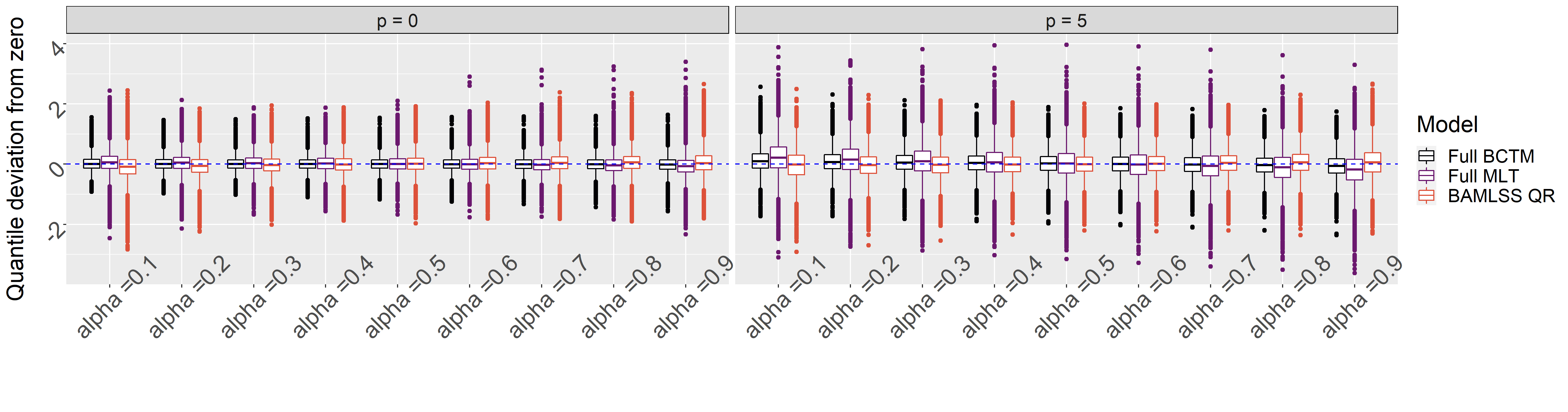
As a second performance measure, we computed conditional quantiles of the fitted response distribution corresponding to a sequence of probabilities $\alpha$ via numerical inversion. Fig. 2 shows the deviations of these from their true counterparts together with similar results obtained via QR BAMLSS which was used as a benchmark.

Third, as a measure of accuracy that concentrates on tail features of the distribution, Fig. 3 shows the quantile score function $\text{QS}_{\alpha}(F^{-1}(\alpha),y)=2(\mathcal{I}(y<F^{-1}(\alpha))-\alpha)(\alpha-y)$ at $\alpha=0.05$ and $\alpha=0.95$, where $\mathcal{I}(A)$ = 1 if $A$ is true, and zero otherwise (Gneiting 2011). Last, to measure the overall forecast accuracy, we plot the decomposition of the continuous ranked probability score (Laio and Tamea 2007, CRPS;) which can be written as $\text{CRPS}(F,y)=\int_{0}^{1}\text{QS}_{\alpha}(F{-1}(\alpha),y)\mathrm{d}\alpha$ in Fig. 4. Both, the QS and CRPS are based on the prediction grids used for the MAD and lower values suggest greater accuracy.

To compare BCTM and MLT from a different perspective, we consider empirical coverage rates of pointwise $95\%$ credible/confidence intervals in a simulation setting that concentrates on the estimation of nonlinear covariate effects.

The Framingham Heart Study dataset of (Zhang and Davidian 2001) contains the cholesterol levels ($\mathit{cholst}$) of $200$ patients at three to six different measurement points over the course of up to $10$ years along the current $\mathit{age}$ and $\mathit{sex}$ of each individual. There are $n=1044$ observations in total.

We fitted various BCTM specifications that differ in their specific form of the transformation function and the chosen hyperprior. All of them are based on

• •

  $\big(\text{\boldmath$\vartheta$},\Phi,\allowbreak(\text{\boldmath$a$}(y)^{\top}\otimes\allowbreak(1,\mathit{age}),\allowbreak(\mathit{year},\allowbreak\mathit{sex}))^{\top},\pi_{\vartheta}(\text{\boldmath$\vartheta$})\big)$: a response-varying VCM for $\mathit{age}$ and intercept in $\text{\boldmath$a$}(y)$, leading to

  	$\displaystyle\mathbb{P}(\mathit{cholst}\leq y|\text{\boldmath$x$})$	$\displaystyle=\Phi\left(h_{1}(y)+h_{2}(y|\mathit{age})+h_{3}(y|\mathit{year})+h_{4}(y|\mathit{sex})\right)$
  		$\displaystyle=\Phi\left(\text{\boldmath$a$}(y)^{\top}\text{\boldmath$\gamma$}_{1}+\mathit{age}\cdot\bm{a}(y)^{\top}\text{\boldmath$\gamma$}_{2}+\mathit{year}\cdot\gamma_{3}+\mathit{sex}\cdot\gamma_{4}\right).$

• •

  $\big(\text{\boldmath$\vartheta$},\Phi,(\text{\boldmath$a$}(y)^{\top}\otimes\text{\boldmath$b$}(\mathrm{age})^{\top},(\mathit{year},\mathit{sex}))^{\top},\allowbreak\pi_{\vartheta}(\text{\boldmath$\vartheta$})\big)$: a full BCTM for $\mathit{age}$, where $\text{\boldmath$a$}(y)$ and $\text{\boldmath$b$}(\mathit{age})$ contain an intercept, the tensor product is centered around zero and $\text{\boldmath$b$}(\mathit{age})$ consists of a 10-dimensional B-splines basis leading to

  	$\displaystyle\mathbb{P}(\mathit{cholst}\leq y|\text{\boldmath$x$})$	$\displaystyle=\Phi\left(h_{1}(y|\mathit{age})+h_{2}(y|\mathit{year})+h_{3}(y|\mathit{sex})\right)$
  		$\displaystyle=\Phi\left((\text{\boldmath$a$}(y)^{\top}\otimes\text{\boldmath$b$}_{1}(\mathit{age})^{\top})^{\top}\text{\boldmath$\gamma$}_{1}+\mathit{year}\cdot\gamma_{2}+\mathit{sex}\cdot\gamma_{3}\right).$

References

- (1)
- Andrinopoulou et al. (2018) Andrinopoulou, E.-R., Eilers, P. H., Takkenberg, J. J. and Rizopoulos, D. (2018). Improved dynamic predictions from joint models of longitudinal and survival data with time-varying effects using P-splines, Biometrics 74(2): 685–693.
- Betancourt (2017) Betancourt, M. (2017). Conceptual intro to Hamiltonian Monte Carlo, arXiv:1701.02434 .
- Box and Cox (1964) Box, G. E. and Cox, D. R. (1964). An analysis of transformations, Journal of the Royal Statistical Society: Series B (statistical methodology) 26(2): 211–243.
- Carlan and Kneib (2022) Carlan, M. and Kneib, T. (2022). Bayesian discrete conditional transformation models, arXiv e-prints p. arXiv:2205.08594.
- Cheng et al. (1995) Cheng, S., Wei, L. and Ying, Z. (1995). Analysis of transformation models with censored data, Biometrika 82(4): 835–845.
- Chernozhukov et al. (2013) Chernozhukov, V., Fernández-Val, I. and Melly, B. (2013). Inference on counterfactual distributions, Econometrica 81(6): 2205–2268.
- Eddelbuettel and Balamuta (2017) Eddelbuettel, D. and Balamuta, J. J. (2017). Extending R with C++: A Brief Introduction to Rcpp, PeerJ Preprints 5: e3188v1.
- Gneiting (2011) Gneiting, T. (2011). Quantiles as optimal point forecasts, International Journal of forecasting 27(2): 197–207.
- Hastie and Tibshirani (1990) Hastie, T. J. and Tibshirani, R. J. (1990). Generalized additive models, Vol. 43, CRC press.
- Henderson et al. (2002) Henderson, R., Shimakura, S. and Gorst, D. (2002). Modeling spatial variation in leukemia survival data, Journal of the American Statistical Association 97(460): 965–972.
- Hoffman and Gelman (2014) Hoffman, M. D. and Gelman, A. (2014). The No-U-Turn Sampler: adaptively setting path lengths in Hamiltonian Monte Carlo., Journal of Machine Learning Research 15(1): 1593–1623.
- Horowitz and Lee (2005) Horowitz, J. L. and Lee, S. (2005). Nonparametric estimation of an additive quantile regression model, Journal of the American Statistical Association 100(472): 1238–1249.
- Hothorn (2017) Hothorn, T. (2017). mlt: Most likely transformations. r package vignette version 0.2-0.
- Hothorn (2022) Hothorn, T. (2022). tram: Transformation models. R package vignette version 0.7-0.
- Hothorn et al. (2014) Hothorn, T., Kneib, T. and Bühlmann, P. (2014). Conditional transformation models, Journal of the Royal Statistical Society: Series B (Statistical Methodology) 76(1): 3–27.
- Hothorn et al. (2018) Hothorn, T., Möst, L. and Bühlmann, P. (2018). Most likely transformations, Scandinavian Journal of Statistics 45(1): 110–134.
- James et al. (2021) James, N. T., Harrell, F. E. and Shepherd, B. E. (2021). Bayesian cumulative probability models for continuous and mixed outcomes, arXiv:2102.00330 .
- Klein and Kneib (2016) Klein, N. and Kneib, T. (2016). Scale-dependent priors for variance parameters in structured additive distributional regression, Bayesian Analysis 11(4): 1071–1106.
- Klein, Kneib, Klasen and Lang (2015) Klein, N., Kneib, T., Klasen, S. and Lang, S. (2015). Bayesian structured additive distributional regression for multivariate responses, Journal of the Royal Statistical Society. Series C: Applied Statistics 64(4): 569–591.
- Klein, Kneib, Lang, Sohn et al. (2015) Klein, N., Kneib, T., Lang, S., Sohn, A. et al. (2015). Bayesian structured additive distributional regression with an application to regional income inequality in Germany, The Annals of Applied Statistics 9(2): 1024–1052.
- Kneib et al. (2019) Kneib, T., Klein, N., Lang, S. and Umlauf, N. (2019). Modular regression-a lego system for building structured additive distributional regression models with tensor product interactions, Test 28(1): 1–39.
- Koenker and Bassett (1978) Koenker, R. and Bassett, G. (1978). Regression quantiles, Econometrica 46: 33–50.
- Laio and Tamea (2007) Laio, F. and Tamea, S. (2007). Verification tools for probabilistic forecasts of continuous hydrological variables, Hydrology and Earth System Sciences 11(4): 1267–1277.
- Lang and Brezger (2004) Lang, S. and Brezger, A. (2004). Bayesian P-splines, Journal of Computational and Graphical Statistics 13(1): 183–212.
- Linton et al. (2008) Linton, O., Sperlich, S., Van Keilegom, I. et al. (2008). Estimation of a semiparametric transformation model, The Annals of Statistics 36(2): 686–718.
- Mallick and Walker (2003) Mallick, B. K. and Walker, S. (2003). A Bayesian semiparametric transformation model incorporating frailties, Journal of Statistical Planning and Inference 112(1-2): 159–174.
- McKay Curtis and Ghosh (2011) McKay Curtis, S. and Ghosh, S. K. (2011). A variable selection approach to monotonic regression with Bernstein polynomials, Journal of Applied Statistics 38(5): 961–976.
- Michaelis et al. (2018) Michaelis, P., Klein, N. and Kneib, T. (2018). Bayesian multivariate distributional regression with skewed responses and skewed random effects, Journal of Computational and Graphical Statistics 27(3): 602–611.
- Monnahan and Kristensen (2018) Monnahan, C. C. and Kristensen, K. (2018). No-U-Turn Sampling for fast Bayesian inference in ADMB and TMB: Introducing the adnuts and tmbstan R packages., PLoS ONE 13(5): e0197954.
- Möst (2015) Möst, L. (2015). Conditional Transformation Models-Interpretable Parametrisations and Censoring, Verlag Dr. Hut.
- Neal et al. (2011) Neal, R. M. et al. (2011). MCMC using Hamiltonian dynamics, in S. Brooks, A. Gelman, G. Jones and X.-L. Meng (eds), Handbook of Markov chain Monte Carlo, 1st edn, Chapman & Hall/CRC, New York, chapter 5, pp. 133–162.
- Nelder and Wedderburn (1972) Nelder, J. A. and Wedderburn, R. W. (1972). Generalized linear models, Journal of the Royal Statistical Society: Series A (General) 135(3): 370–384.
- Nesterov (2009) Nesterov, Y. (2009). Primal-dual subgradient methods for convex problems, Mathematical programming 120(1): 221–259.
- Papaspiliopoulos et al. (2007) Papaspiliopoulos, O., Roberts, G. O. and Sköld, M. (2007). A general framework for the parametrization of hierarchical models, Statistical Science 22(1): 59–73.
- Pericchi (1981) Pericchi, L. (1981). A Bayesian approach to transformations to normality, Biometrika 68: 35–43.
- Politis (2013) Politis, D. N. (2013). Model-free model-fitting and predictive distributions, Test 22(2): 183–221.
- Pya (2010) Pya, N. (2010). Additive models with shape constraints, PhD thesis, University of Bath.
- Pya and Wood (2015) Pya, N. and Wood, S. N. (2015). Shape constrained additive models, Statistics and Computing 25(3): 543–559.
- R Core Team (2020) R Core Team (2020). R: A Language and Environment for Statistical Computing, R Foundation for Statistical Computing, Vienna, Austria.
- Rigby and Stasinopoulos (2005) Rigby, R. A. and Stasinopoulos, D. M. (2005). Generalized additive models for location, scale and shape, Journal of the Royal Statistical Society: Series C (Applied Statistics) 54(3): 507–554.
- Rue and Held (2005) Rue, H. and Held, L. (2005). Gaussian Markov Random Fields: Theory and Applications, CRC.
- Song and Lu (2012) Song, X.-Y. and Lu, Z.-H. (2012). Semiparametric transformation models with Bayesian P-splines, Statistics and Computing 22(5): 1085–1098.
- Spiegelhalter et al. (2002) Spiegelhalter, D. J., Best, N. G., Carlin, B. P. and Van Der Linde, A. (2002). Bayesian measures of model complexity and fit, Journal of the Royal Statistical Society: Series B (Statistical Methodology) 64(4): 583–639.
- Tamási and Hothorn (2022) Tamási, B. and Hothorn, T. (2022). tramME: Mixed-effects transformation models using template model builder, R Journal pp. Epub–ahead.
- Tang et al. (2018) Tang, N., Wu, Y. and Chen, D. (2018). Semiparametric Bayesian analysis of transformation linear mixed models, Journal of Multivariate Analysis 166: 225–240.
- Umlauf et al. (2018) Umlauf, N., Klein, N. and Zeileis, A. (2018). BAMLSS: Bayesian additive models for location, scale, and shape (and beyond), Journal of Computational and Graphical Statistics 27: 612–627.
- Waldmann et al. (2013) Waldmann, E., Kneib, T., Yue, Y. R., Lang, S. and Flexeder, C. (2013). Bayesian semiparametric additive quantile regression, Statistical Modelling 13(3): 223–252.
- Walker and Mallick (1999) Walker, S. and Mallick, B. K. (1999). A Bayesian semiparametric accelerated failure time model, Biometrics 55(2): 477–483.
- Watanabe (2010) Watanabe, S. (2010). Asymptotic equivalence of Bayes cross validation and widely applicable information criterion in singular learning theory, Journal of Machine Learning Research 11(Dec): 3571–3594.
- Yu and Moyeed (2001) Yu, K. and Moyeed, R. A. (2001). Bayesian quantile regression, Statistics & Probability Letters 54(4): 437–447.
- Zhang and Davidian (2001) Zhang, D. and Davidian, M. (2001). Linear mixed models with flexible distributions of random effects for longitudinal data, Biometrics 57(3): 795–802.
- Zhou et al. (2020) Zhou, H., Hanson, T. and Zhang, J. (2020). spBayesSurv: Fitting Bayesian spatial survival models using R, Journal of Statistical Software 92(9): 1–33.