On a length-biased Birnbaum-Saunders regression model applied to meteorological data
Abstract
The length-biased Birnbaum-Saunders distribution is both useful and practical for environmental sciences. In this paper, we initially derive some new properties for the length-biased Birnbaum-Saunders distribution, showing that one of its parameters is the mode and that it is bimodal. We then introduce a new regression model based on this distribution. We implement use the maximum likelihood method for parameter estimation, approach interval estimation and consider three types of residuals. An elaborate Monte Carlo study is carried out for evaluating the performance of the likelihood-based estimates, the confidence intervals and the empirical distribution of the residuals. Finally, we illustrate the proposed regression model with the use of a real meteorological data set.
Keywords. Length-biased model; Mode regression; Bimodality; Monte Carlo simulation; Meteorological data.
1 Introduction
Birnbaum-Saunders (BS) regression models have been widely used in the literature; see the literature review by Balakrishnan and Kundu, 2019. Recently, Dasilva et al., 2020 performed a comparison of three existing regression approaches, studied by Rieck and Nedelman, 1991, Leiva et al., 2014 and Balakrishnan and Zhu, 2015, to deal with the modeling of asymmetric data following the BS distribution. Other recent studies involving BS regression models can be seen in Sánchez et al., 2020a; Sánchez et al., 2020b and Leiva et al., 2020.
Length-biased distributions are special cases of weighted distributions; see Sansgiry and Akman, 2001. In the area of environmental sciences, as noted by Patil, 2006, the use of weighted distributions is more adequade, since observations from this area fall in the nonexperimental, nonreplicated, and nonrandom categories. Weighted distributions take into account these caracteristichcs by providing probability-adjusted models that consider the method of ascertainment; see Patil, 2006.
In the context of BS models, Leiva et al., 2009 proposed a length-biased version of the BS (LBS) distribution. The authors provided moments and some properties of this distribution, which was illustrated with real data related to water quality. Nevertheless, no regression model based on the LBS distribution has been proposed in the literature. Therefore, the primary objective of this paper is to propose a regression model based on the LBS distribution. The secondary objectives are: (i) to investigate some properties of the LBS distribution, such as bimodality and mode; (ii) to obtain point and interval estimates of the model parameters; (iii) to carry out Monte Carlo simulations to evaluate the performance of the estimates; and (iv) to discuss a real data application of the proposed methodology.
The rest of this paper proceeds as follows. In Section 2, we describe briefly the LBS distribution proposed by Leiva et al., 2009 and present some novel properties of this model. In Section 3, we formulate the regression model based on the LBS distribution, and then detail the associated point and interval estimation and residual analysis. In Section 4, we carry out Monte Carlo simulations, and an illustration with a meteorological data is done in Section 5. Finally, in Section 6, we discuss conclusions and some possible future research in this topic.
2 The LBS distribution and some novel properties
In this section, we briefly describes the LBS distribution. Then, some novel results on bimodality and monotonicity of the hazard rate (HR) of the LBS distribution are obtained.
2.1 The LBS distribution
Let be a positive random variable with probability density function (PDF) . Then, the length-biased version of , denoted by , has PDF
| (2.1) |
provided the expectation exists. In the case of the LBS distribution, the random variable follows a BS distribution (Birnbaum and Saunders, 1969) with shape parameter and scale parameter , denoted by , with . Thus, is a random variable following a LBS distribution with PDF given by
| (2.2) |
with , and . In this case, we write . According to Leiva et al., 2009, the parameter in (2.2) relates only to the scale, while the parameter controls asymmetry and kurtosis of the distribution. In Subsection 2.2, we prove that the parameter is the mode when and the distribution is bimodal when ; Figure 1 displays different shapes of the LBS PDF for different combinations of parameters.


Let ; we then readily have the following properties (Leiva et al., 2009): (P1) , with ; (P2) ; (P3) ; (P4) , where ; and (P5) has PDF , where , and .
2.2 Novel properties
2.2.1 Bimodality properties
In order to state and prove the main result of this subsection (Theorem 2.2), we define the following function
| (2.3) |
Notice that the -th derivative of , denoted by , satisfies (or ) for odd (or even), where . Some special cases of these derivatives, when , are of the following form:
Proposition 2.1 (Modes).
A mode of the LBS distribution is obtained by resolving the following cubic equation
Proof.
Let . A simple computation shows that the th derivative of is given by
| (2.5) |
where and we are denoting . Since
| (2.6) |
by combining (2.5) and (2.6) we have
By using (2.3), (2.2.1) and simple algebraic manipulations we get that if and only if
Therefore, a mode of the LBS distribution must satisfy the above equation.
∎
The next theorem reveals that the parameter of the LBS distribution, in addition to controlling asymmetry, controls the uni- or bimodal shape of the distribution regardless of the parameter .
Theorem 2.2 (Unimodality and Bimodality).
The PDF of the LBS distribution (2.2) has the following shapes:
- 1)
It is unimodal as , with mode ;
- 2)
It is bimodal as , with modes
(2.7) and with minimum point .
Proof.
By Proposition 2.1, a mode of the LBS distribution satisfies the following cubic equation
| (2.8) |
By using Descartes’ rule of signs (see, e.g. Xue, 2000) in (2.8), we have the following statements:
- a)
has exactly one positive root when ;
- b)
has three or one positive roots when .
On the other hand, it is well-known that the discriminant of a cubic polynomial is given by . In our case, we have
Hence, the following statements with respect to follow:
- c)
when . By using a) and b), this implies that has exactly one positive root and two complex conjugate non-real roots;
- d)
when . By using a) and b), this implies that, has exactly one positive triple root;
- e)
when . By using a) and b), this implies that, has three distinct positive roots.
We are now ready to prove Items 1) and 2). Indeed, note that is a critical point of the LBS density , , because . Then, since and , Items c) and d) imply the statement in Item 1); and Item e) implies that the LBS density is bimodal as whenever is a minimum point. To complete the proof of Item 2), it remains to show that, when ,
- (I)
is a minimum point for the LBS density, and that
- (II)
the modes of the LBS density are given by defined in (2.7).
To verify Item (I), it is sufficient to check that when . Indeed, note that
| (2.9) |
and that
Substituting (2.9) in the above equation we have
By using the relations , , and the expressions for the derivatives of given in (2.2.1), we get
whenever . Then the statement in Item (I) follows.
In what remains of the proof we check Item (II). Indeed, since is a critical point for the LBS density, note the cubic equation (2.8) can be written as
| (2.10) |
Bhaskara’s Formula gives the following roots for :
Since and, and , the proof of Item (II) follows. We thus complete the proof of Item 2).
∎
2.2.2 Some properties of the HR of the LBS distribution
The survival function (SF) and HR of the LBS distribution are given respectively by
| (2.11) | ||||
where , and
| (2.12) | ||||
with and being the standard normal PDF and cumulative distribution function (CDF), respectively.
To enunciate and prove the following two results, we follow the same notations as Theorem 2.2.
Proposition 2.3 (Monotonicity of HR, case ).
The HR of the LBS distribution with has the following monotonic properties:
- 1)
It is increasing for all ;
- 2)
It is decreasing for all , for some .
Proof.
When the LBS density is unimodal with mode (Theorem 2.2). Then there is so that the LBS density is a concave upward function on the interval . In other words, for all . Equivalently, the function decreases on . But since, by unimodality, the LBS density decreases on this interval, we have that the function , defined as
decreases for all , because , , is a product of nonnegative decreasing functions. Hence, by Glaser, 1980 the function is decreasing for all . This proves the second item.
In what follows we prove Item 1). Indeed, by unimodality of the LBS density (Theorem 2.2), the LBS dentity increases on . Hence, since the SF , , is decreasing, by definition of HR it follows that is a product of nonnegative increasing functions. Therefore, it is a increasing function for all .
∎
Proposition 2.4 (Monotonicity of HR, case ).
The HR of the LBS distribution with has the following monotonic properties:
- 1)
It is increasing for all ou for all ;
- 2)
It is decreasing for all ou for all , for some and .
3 The LBS regression model
In this section, we formulate the LBS regression model, and then detail the associated estimation, inference and residual analysis based on the maximum likehood method.
3.1 The model and maximum likelihood estimation
Let denote independent random variables, where , with observed values denoted by , respectively. Then, the LBS regression model is formulated as
| (3.1) |
where and are vectors of unknown parameters, with , and . The vectors and are known covariates from the -th row of the matrices and which are full rank, i.e., and . Commonly and , where is a 1’s vector size . The link function is invertible and at least twice differentiable. Usually (log function) and (square root function).
The corresponding likelihood function for is
| (3.2) |
where is the LBS PDF given in (2.2). By taking the logarithm in (3.2), we obtain the log-likelihood function for as
| (3.3) |
where and , as defined in (3.1).
The maximum likelihood estimators of the LBS regression model parameters are the solution of the equation , where is the gradient vector, with the first derivatives given by
| (3.4) |
with
| (3.5) | ||||
where , , , , and .
However, these equations do not have a closed form, requiring the use of iterative numerical methods to solve them. They are solved using the BFGS quasi-Newton method; see Mittelhammer et al., 2000[p. 199]. Under regularity conditions (Cox and Hinkley, 1974), the asymptotic distribution of is a multivariate normal, that is,
| (3.6) |
where denotes convergence in distribution and is the asymptotic covariance matrix of , which is the inverse of the expected Fisher information matrix. One can approximate the expected Fisher information matrix by its observed version obtained from the Hessian matrix , such that . The standard errors (SEs) can then be approximated by the square roots of the diagonal elements in the covariance matrix evaluated at . Note that
| (3.7) |
with
| (3.8) | ||||
where , , , , , , , , and .
3.2 Initial values
The initial value for can be obtained by the use of least squares method from
| (3.9) |
where and is the link function.
Let for . Then, the initial value for can be estimated by ordinary least squares, as
| (3.10) |
where , and is the link function.
3.3 Confidence intervals
In this subsection, we derive some confidence intervals (CIs) using the asymptotic properties of maximum likelihood estimators and the bootstrap approach.
3.3.1 Asymptotic confidence interval
Based on the asymptotic normal approximation in (3.6), we have the asymptotic CI (ACI) for the parameter as
| (3.11) |
where is the quantile of the standard normal distribution, and .
3.3.2 Bootstrap confidence intervals
The bootstrap approach, developed by Efron and Tibshirani, 1986, provides another way to obtain CIs. We compute the percentile bootstrap CI (PCI) and the bias-corrected and accelerated CI (BCI) for the parameter , with , based on the the following steps:
- (i)
Use the maximum likelihood method to obtain an estimate of from the original sample, and then estimate the components , with .
- (ii)
For each bootstrap replica :
- (a)
For each , draw a pseudo-random sample , where , as defined in (2.2).
- (b)
Compute the -th replica of by the maximum likelihood method based on the pseudo-sample generated in (a).
- (a)
3.4 Residual analysis
We perform residuals analysis in order to evaluate the validity of the assumptions of the model and also as tools for model selection. We consider three types of residuals. The first residual is the generalized Cox-Snell (GCS), given by
| (3.12) |
where is the survival function fitted to the data. The GCS residual is asymptotically standard exponential, in short, when the model is correctly specified whatever the specification of the model is;
The second residual is the randomized quantile (RQ), given by
| (3.13) |
where is the inverse function of the standard normal CDF and is the survival function fitted to the data. The RQ residual follows a standard normal distribution when the model is specified correctly, regardless of the LBS model.
The third residual (U) is based on the relationship given by (P5) of Subsection 2.1. Note that
| (3.14) |
should result in being independent and identically distributied observations from a mixture of two gamma distributions; see (P5). Thus, from the given data, we may estimate and by and , respectively, and use them to determine the values.
4 Monte Carlo simulation studies
Three Monte Carlo simulation studies are carried out to evaluate the performances of the maximum likelihood estimates, the coverage probabilities of the 95% CIs and the empirical distribution of the residuals. We use the R software to do all numerical calculations; see R Core Team, 2020.
The simulation scenario considers sample size . For the component, the values of the true parameters are taken as and . For the component, we consider the scenario with and without covariates. For the scenario without covariates, and for the scenario with covariates, and . The covariates and in the predictors of the (3.1) models were obtained from a uniform distribution in the interval . We use 5,000 Monte Carlo replications for each combination of above given parameters and sample size; we use bootstrap replicates.
4.1 Maximum likelihood estimates
The maximum likelihood estimation results for the considered LBS regresion model are presented in Tables 1 and 2. The empirical mean, bias and mean squared error (MSE) are reported. The results of Tables 1 and 2 allow us to conclude that, when the sample size increases, the empirical means tend to the reference true parameter values. Moreover, the empirical bias and MSE both decrease, as expected, when the sample size increases.
| True value | Mean | Bias | MSE | ||||||
|---|---|---|---|---|---|---|---|---|---|
| 50 | 100 | 500 | 50 | 100 | 500 | 50 | 100 | 500 | |
| 1.0049 | 1.0030 | 1.0005 | 0.0049 | 0.0030 | 0.0005 | 0.0032 | 0.0016 | 0.0003 | |
| -1.0009 | -0.9991 | -1.0006 | -0.0009 | 0.0009 | -0.0006 | 0.0086 | 0.0038 | 0.0007 | |
| -1.0438 | -1.0221 | -1.0042 | -0.0438 | -0.0221 | -0.0042 | 0.0128 | 0.0056 | 0.0010 | |
| 0.2691 | 0.2550 | 0.2517 | 0.0191 | 0.0050 | 0.0017 | 0.0280 | 0.0138 | 0.0025 | |
| 1.0027 | 1.0020 | 1.0001 | 0.0027 | 0.0020 | 0.0001 | 0.0021 | 0.0011 | 0.0002 | |
| -1.0011 | -0.9996 | -1.0006 | -0.0011 | 0.0004 | -0.0006 | 0.0056 | 0.0028 | 0.0005 | |
| -1.0424 | -1.0215 | -1.0038 | -0.0424 | -0.0215 | -0.0038 | 0.0117 | 0.0052 | 0.0009 | |
| 0.7869 | 0.7639 | 0.7533 | 0.0369 | 0.0139 | 0.0033 | 0.0270 | 0.0129 | 0.0024 | |
| 1.0012 | 1.0012 | 1.0001 | 0.0012 | 0.0012 | 0.0001 | 0.0010 | 0.0006 | 0.0001 | |
| -1.0011 | -1.0000 | -1.0005 | -0.0011 | 0.0000 | -0.0005 | 0.0029 | 0.0016 | 0.0003 | |
| -1.0413 | -1.0210 | -1.0038 | -0.0413 | -0.0210 | -0.0038 | 0.0105 | 0.0047 | 0.0008 | |
| 1.2955 | 1.2695 | 1.2543 | 0.0455 | 0.0195 | 0.0043 | 0.0254 | 0.0119 | 0.0022 | |
From Table 2, we observe that that when assumes values greater than 2, which is the bimodal case (Theorem 2.2), the MSE values are greater for e for , but not for . This result shows that when bimodality is present, the bias and MSE tend to be greater than the unimodal case. However, as the sample size increases, the bias and MSE decrease dramatically.
| True value | Mean | Bias | MSE | ||||||
|---|---|---|---|---|---|---|---|---|---|
| 50 | 100 | 500 | 50 | 100 | 500 | 50 | 100 | 500 | |
| 1.0028 | 1.0017 | 1.0003 | 0.0028 | 0.0017 | 0.0003 | 0.0014 | 0.0007 | 0.0001 | |
| -0.9992 | -0.9991 | -1.0002 | 0.0008 | 0.0009 | -0.0002 | 0.0042 | 0.0018 | 0.0004 | |
| -1.4180 | -1.4035 | -1.3904 | -0.0317 | -0.0173 | -0.0041 | 0.0120 | 0.0053 | 0.0010 | |
| 1.0106 | 1.0064 | 1.0015 | 0.0106 | 0.0064 | 0.0015 | 0.0070 | 0.0035 | 0.0007 | |
| -0.9990 | -0.9983 | -1.0003 | 0.0010 | 0.0017 | -0.0003 | 0.0158 | 0.0067 | 0.0013 | |
| -0.7263 | -0.7112 | -0.6975 | -0.0331 | -0.0181 | -0.0044 | 0.0130 | 0.0058 | 0.0011 | |
| 1.0316 | 1.0233 | 1.0058 | 0.0316 | 0.0233 | 0.0058 | 0.1290 | 0.0274 | 0.0057 | |
| -1.0010 | -0.9976 | -1.0007 | -0.0010 | 0.0024 | -0.0007 | 0.0429 | 0.0180 | 0.0036 | |
| -0.0389 | -0.0235 | -0.0058 | -0.0389 | -0.0235 | -0.0058 | 0.0430 | 0.0113 | 0.0023 | |
| 1.1071 | 0.9653 | 0.9975 | 0.1071 | -0.0347 | -0.0025 | 2.1341 | 1.7120 | 0.1965 | |
| -1.0034 | -0.9977 | -1.0008 | -0.0034 | 0.0023 | -0.0008 | 0.0551 | 0.0230 | 0.0046 | |
| 0.6240 | 0.7026 | 0.6925 | -0.0692 | 0.0094 | -0.0007 | 0.5316 | 0.4185 | 0.0469 | |
| 1.3516 | 1.0837 | 0.9920 | 0.3516 | 0.0837 | -0.0080 | 2.8662 | 2.4906 | 0.3549 | |
| -1.0034 | -0.9976 | -1.0008 | -0.0034 | 0.0024 | -0.0008 | 0.0540 | 0.0225 | 0.0045 | |
| 0.7309 | 0.8710 | 0.9193 | -0.1854 | -0.0453 | 0.0030 | 0.7141 | 0.6094 | 0.0840 | |
4.2 Coverage probabilities
Tables 3 and 4 present the coverage probabilities of 95% CIs presented Subsection 3.3 for the LBS regression model. The results show that the ACI, PCI and BCI coverage probabilities approach the nominal level of 95% when the sample increases, as expected. However, when takes values greater than 2, the ACI, PCI and BCI coverage probabilities are lower than the corresponding nominal value for and for . In general, the BCI has the best performance, which might be due to its characteristics as this method corrects for bias and skewness in the distribution of bootstrap estimates.
| True value | ACI | PCI | BCI | ||||||
|---|---|---|---|---|---|---|---|---|---|
| 50 | 100 | 500 | 50 | 100 | 500 | 50 | 100 | 500 | |
| 92.44 | 93.96 | 94.70 | 91.78 | 93.18 | 94.06 | 91.82 | 93.24 | 93.96 | |
| 92.44 | 94.10 | 95.04 | 92.10 | 93.80 | 94.54 | 92.12 | 93.88 | 94.48 | |
| 91.26 | 93.94 | 95.16 | 84.58 | 89.26 | 93.96 | 83.16 | 88.68 | 93.60 | |
| 93.12 | 94.50 | 94.58 | 92.78 | 94.12 | 94.38 | 92.80 | 93.98 | 94.32 | |
| 92.24 | 93.78 | 94.78 | 91.66 | 93.08 | 94.16 | 91.68 | 93.06 | 94.02 | |
| 91.60 | 94.12 | 95.16 | 91.32 | 93.78 | 94.92 | 91.30 | 93.82 | 94.82 | |
| 91.36 | 93.46 | 94.88 | 83.86 | 89.34 | 94.02 | 82.26 | 88.74 | 93.66 | |
| 92.72 | 94.34 | 94.48 | 91.26 | 93.86 | 94.14 | 90.88 | 93.74 | 93.82 | |
| 92.00 | 93.46 | 94.76 | 91.60 | 93.04 | 94.10 | 91.62 | 92.74 | 94.12 | |
| 91.32 | 93.80 | 95.08 | 91.06 | 93.66 | 94.72 | 90.90 | 93.44 | 94.54 | |
| 91.60 | 93.30 | 94.76 | 83.36 | 88.80 | 93.78 | 81.66 | 88.12 | 93.70 | |
| 92.68 | 94.02 | 94.52 | 89.50 | 92.50 | 93.94 | 89.04 | 92.56 | 93.82 | |
| True value | ACI | PCI | BCI | ||||||
|---|---|---|---|---|---|---|---|---|---|
| 50 | 100 | 500 | 50 | 100 | 500 | 50 | 100 | 500 | |
| 93.96 | 94.98 | 94.84 | 93.22 | 94.44 | 94.56 | 93.28 | 94.56 | 94.60 | |
| 93.66 | 94.88 | 95.34 | 93.32 | 94.42 | 95.08 | 93.28 | 94.40 | 95.04 | |
| 92.74 | 94.44 | 94.46 | 88.72 | 92.12 | 94.06 | 87.80 | 91.54 | 93.80 | |
| 93.36 | 94.28 | 94.62 | 92.26 | 93.36 | 94.10 | 92.32 | 93.48 | 94.12 | |
| 93.70 | 94.86 | 95.40 | 93.20 | 94.60 | 95.04 | 93.28 | 94.34 | 94.88 | |
| 92.66 | 94.42 | 94.44 | 88.28 | 91.70 | 93.68 | 87.34 | 91.16 | 93.42 | |
| 90.32 | 92.62 | 94.44 | 88.58 | 91.88 | 93.68 | 88.18 | 92.14 | 93.66 | |
| 94.04 | 94.80 | 95.08 | 93.76 | 94.46 | 94.88 | 93.64 | 94.44 | 94.62 | |
| 90.58 | 93.10 | 94.22 | 86.46 | 90.46 | 93.44 | 85.48 | 90.32 | 93.36 | |
| 75.32 | 81.40 | 90.18 | 77.62 | 84.06 | 91.12 | 81.98 | 87.08 | 91.46 | |
| 94.24 | 94.78 | 94.90 | 93.88 | 94.50 | 94.58 | 93.86 | 94.38 | 94.44 | |
| 75.62 | 81.60 | 90.22 | 77.20 | 83.42 | 90.72 | 81.00 | 86.08 | 91.08 | |
| 66.58 | 73.58 | 87.70 | 74.38 | 82.10 | 91.38 | 81.42 | 87.44 | 93.14 | |
| 94.40 | 94.94 | 95.04 | 94.14 | 94.66 | 94.68 | 94.00 | 94.54 | 94.60 | |
| 67.32 | 73.72 | 87.72 | 74.14 | 81.90 | 91.40 | 80.38 | 86.98 | 93.02 | |
4.3 Empirical distribution of residuals
We now present the Monte Carlo simulation results for evaluating the performance of the , and residuals. Tables 6 and 7 presents the empirical mean, standard deviation (SD), coefficient of skewness (CS) and coefficient of kurtosis (CK), whose values are expected to be as in Table 5, for the , and residuals. From Tables 6 and 7, we note that as the sample size increases, the values of the empirical mean, SD, CS and CK approach these values of the reference distributions shown in Table 5. Therefore, the considered residuals conform well with the reference distributions.
| Measure | |||
|---|---|---|---|
| Mean | 1 | 0 | |
| SD | 1 | 1 | |
| CS | 2 | 0 | |
| CK | 9 | 3 |
| Statistic | |||||||||
|---|---|---|---|---|---|---|---|---|---|
| 50 | 100 | 500 | 50 | 100 | 500 | 50 | 100 | 500 | |
| Mean | 0.9999 | 1.0000 | 0.9999 | -0.0011 | -0.0002 | -0.0001 | 1.1256 | 1.1270 | 1.1307 |
| SD | 0.9775 | 0.9904 | 0.9969 | 1.0092 | 1.0048 | 1.0009 | 1.4916 | 1.5369 | 1.5728 |
| CS | 1.5475 | 1.7426 | 1.9310 | 0.0378 | 0.0123 | 0.0058 | 2.0560 | 2.3326 | 2.6393 |
| CK | 5.6464 | 6.8645 | 8.3488 | 2.7956 | 2.8948 | 2.9781 | 7.7884 | 9.8548 | 12.8408 |
| Mean | 1.0012 | 1.0006 | 1.0004 | -0.0035 | -0.0013 | -0.0008 | 1.1640 | 1.1602 | 1.1659 |
| SD | 0.9771 | 0.9904 | 0.9970 | 1.0064 | 1.0037 | 1.0005 | 1.5345 | 1.5755 | 1.6134 |
| CS | 1.5528 | 1.7473 | 1.9316 | 0.0324 | 0.0101 | 0.0052 | 2.0458 | 2.3172 | 2.6102 |
| CK | 5.6805 | 6.8971 | 8.3551 | 2.7995 | 2.8997 | 2.9790 | 7.7461 | 9.7546 | 12.5849 |
| Mean | 1.0019 | 1.0010 | 1.0004 | -0.0051 | -0.0020 | -0.0008 | 1.2384 | 1.2286 | 1.2359 |
| SD | 0.9770 | 0.9906 | 0.9970 | 1.0040 | 1.0026 | 1.0004 | 1.6149 | 1.6505 | 1.6894 |
| CS | 1.5618 | 1.7542 | 1.9334 | 0.0275 | 0.0074 | 0.0048 | 2.0176 | 2.2776 | 2.5478 |
| CK | 5.7339 | 6.9420 | 8.3706 | 2.8089 | 2.9064 | 2.9803 | 7.6149 | 9.5076 | 12.0720 |
| Statistic | |||||||||
|---|---|---|---|---|---|---|---|---|---|
| 50 | 100 | 500 | 50 | 100 | 500 | 50 | 100 | 500 | |
| Mean | 1.0013 | 1.0011 | 1.0005 | -0.0013 | -0.0012 | -0.0006 | 1.0581 | 1.0591 | 1.0602 |
| SD | 0.9964 | 0.9975 | 0.9994 | 1.0099 | 1.0048 | 1.0009 | 1.4512 | 1.4703 | 1.4893 |
| CS | 1.6539 | 1.7915 | 1.9457 | -0.0011 | -0.0004 | -0.0006 | 2.1920 | 2.4287 | 2.7033 |
| CK | 6.1768 | 7.1628 | 8.4571 | 2.8832 | 2.9342 | 2.9822 | 8.5821 | 10.5504 | 13.4125 |
| Mean | 1.0003 | 1.0002 | 1.0000 | 0.0001 | 0.0001 | 0.0000 | 1.2130 | 1.2168 | 1.2208 |
| SD | 0.9946 | 0.9963 | 0.9989 | 1.0102 | 1.0051 | 1.0010 | 1.6337 | 1.6556 | 1.6774 |
| CS | 1.6453 | 1.7866 | 1.9453 | 0.0038 | 0.0024 | 0.0004 | 2.1283 | 2.3365 | 2.5793 |
| CK | 6.1364 | 7.1363 | 8.4548 | 2.8744 | 2.9293 | 2.9813 | 8.2144 | 9.9125 | 12.3395 |
| Mean | 0.9998 | 0.9999 | 1.0000 | 0.0017 | 0.0008 | 0.0002 | 1.6375 | 1.6492 | 1.6622 |
| SD | 0.9897 | 0.9931 | 0.9981 | 1.0113 | 1.0056 | 1.0011 | 1.9901 | 2.0168 | 2.0452 |
| CS | 1.6113 | 1.7636 | 1.9391 | 0.0239 | 0.0151 | 0.0036 | 1.8374 | 1.9877 | 2.1610 |
| CK | 5.9778 | 7.0118 | 8.4133 | 2.8428 | 2.9130 | 2.9777 | 6.7649 | 7.8887 | 9.3977 |
| Mean | 0.9977 | 0.9986 | 0.9997 | 0.0126 | 0.0077 | 0.0018 | 2.1833 | 2.2628 | 2.3194 |
| SD | 0.9832 | 0.9895 | 0.9972 | 1.0274 | 1.0158 | 1.0036 | 2.2428 | 2.2937 | 2.3419 |
| CS | 1.5768 | 1.7413 | 1.9332 | 0.0953 | 0.0576 | 0.0132 | 1.5351 | 1.6346 | 1.7486 |
| CK | 5.8354 | 6.9030 | 8.3785 | 2.8490 | 2.9029 | 2.9698 | 5.5880 | 6.3225 | 7.2565 |
| Mean | 0.9972 | 0.9982 | 0.9996 | 0.0106 | 0.0060 | 0.0017 | 2.2528 | 2.3701 | 2.4905 |
| SD | 0.9751 | 0.9830 | 0.9959 | 1.0262 | 1.0147 | 1.0039 | 2.2443 | 2.3079 | 2.3808 |
| CS | 1.5659 | 1.7324 | 1.9311 | 0.1321 | 0.0872 | 0.0224 | 1.5002 | 1.5872 | 1.6827 |
| CK | 5.8005 | 6.8689 | 8.3697 | 2.9153 | 2.9578 | 2.9848 | 5.4820 | 6.1538 | 6.9842 |
5 Application to real data
In this section, the LBS regression model is illustrated using data from the Meteorological Database for Teaching and Research (BDMEP) for the years 2011-2016, from the Brazilian National Institute of Meteorology (INMET) (Source: INMET Network Data). The dependent variable () is water evaporation . The covariates considered in the study were: is the actual evapotranspiration (mm); is the total insolation (h); is the cloudiness (tenths); and is the relative humidity (%). The evaporation is measured by the piche evaporimeter, all monthly averages, observed at a monitoring station located in Brasília, Brazil. Other environmental variables were considered in an initial analysis, however only the afore-mentioned variables were considered statistically significant, at the 5% level of significance, thus remaining in the final model adopted in this application.
Regarding the dependent variable, water evaporation, the actual evapotranspiration, cloudiness and relative humidity variables have a negative correlation of -0.55 and -0.74, -0.97, respectively, while the total insolation variable has a positive correlation (0.77). Therefore, in general, the lower the levels of actual evapotranspiration, cloudiness and relative humidity in the environment, the greater the water evaporation. On the other hand, the greater the total insolation, the greater the amount of water evaporation. These results are in line with what was expected in the environment.
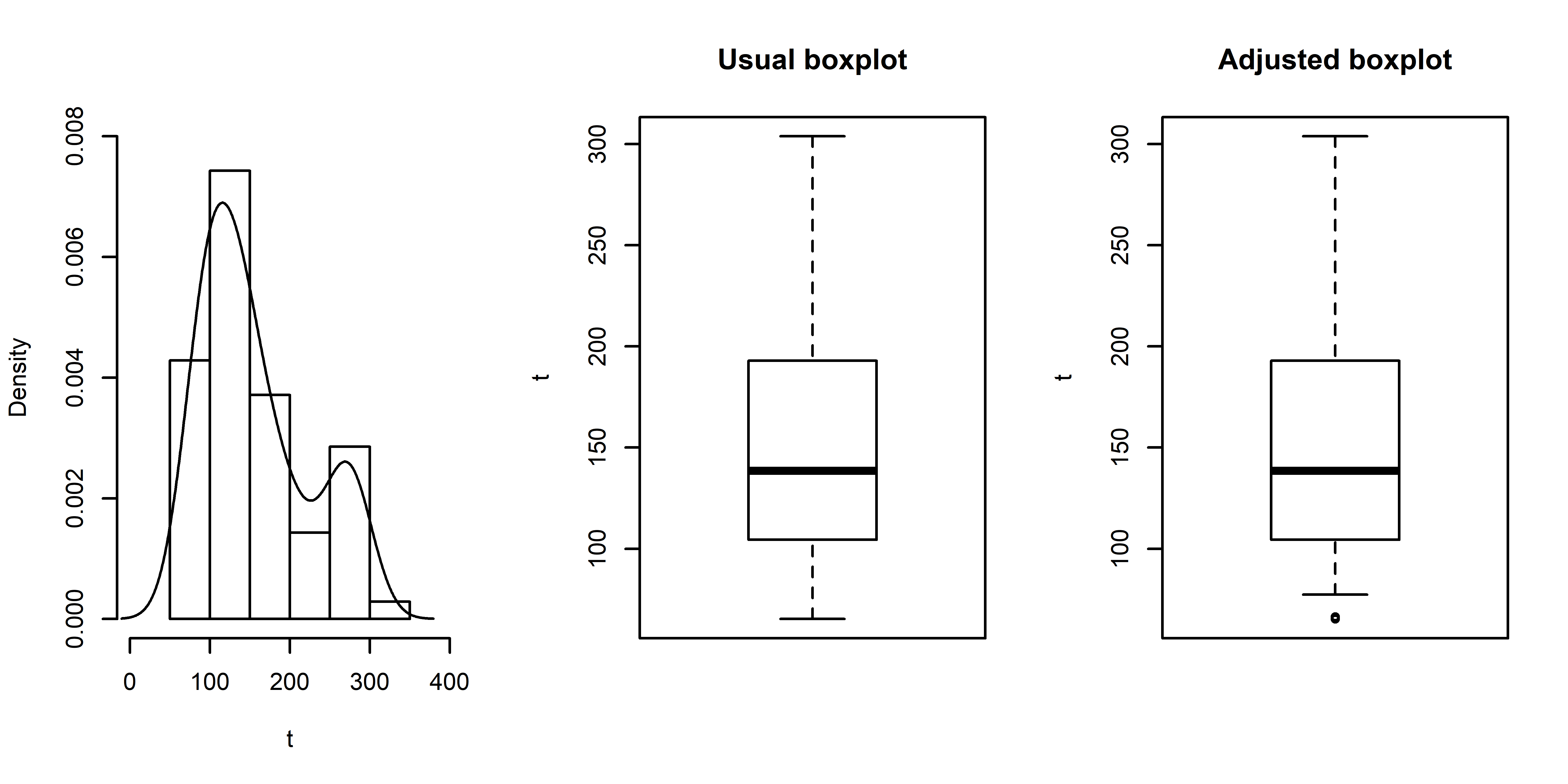
Table 8 reports descriptive statistics of the observed water evaporation, including the minimum, median, mean, maximum, SD, coefficient of variation (CV), CS and CK values. From this table, we observe a skewed and high kurtosis features in the data.
| Variable | Min. | Median | Mean | Max. | SD | CV (%) | CS | CK | |
|---|---|---|---|---|---|---|---|---|---|
| Water evaporation | 70 | 65.3 | 138.55 | 156.88 | 303.80 | 66.68 | 42.50 | 0.73 | -0.67 |
Figure 2 presents an estimated density superimposed on the histogram and boxplots for the water evaporation data. The adjusted boxplot for the water evaporation data indicates that some outliers are not identified by the usual boxplot; see Figure 2(right). The adjusted boxplot is used when the data is skew distributed; see Hubert and Vandervieren, 2008. Note that the skewness observed in Table 8 is confirmed by the histogram presented in Figure 2(left); this figure also indicates bimodality. Thus, the LBS regression model seems to be appropriate to describe these data.
We analyze the water evaporation data using the LBS regression model, expressed as
| (5.1) | ||||
Table 9 reports the maximum likelihood estimates, computed by the BFGS quasi-Newton method, SEs and 95% CI estimates. Note that the 95% CIs do not include the null value (except the intercept for the component), then the coefficients are statistically significant.
| Point Estimation | Interval estimation | ||||
| Estimates | ACI | PCI | BCI | ||
| components | |||||
| (Intercept) | 6.7430 (0.1723) | (6.4052, 7.0808) | (6.4009, 7.0722) | (6.3994, 7.0692) | |
| Actual evapotranspiration () | 0.0015 (0.0004) | (0.0007, 0.0023) | (0.0008, 0.0023) | (0.0007, 0.0023) | |
| Total insolation () | 0.0011 (0.0005) | (0.0002, 0.0020) | (0.0002, 0.0020) | (0.0002, 0.0020) | |
| Cloudiness () | 0.0434 (0.0152) | (0.0136, 0.0732) | (0.0166, 0.0742) | (0.0178, 0.0744) | |
| Relative humidity () | -0.0366 (0.0010) | (-0.0386, -0.0346) | (-0.0386, -0.0345) | (-0.0387, -0.0346) | |
| components | |||||
| (Intercept) | 1.0396 (1.4433) | (-1.7892, 3.8683) | (-2.7158, 4.8980) | (-2.8676, 4.7398) | |
| Total insolation () | -0.0130 (0.0042) | (-0.0212, -0.0048) | (-0.0250, -0.0028) | (-0.0247, -0.0026) | |
| Cloudiness () | -0.2324 (0.1117) | (-0.4513, -0.0135) | (-0.5124, 0.0430) | (-0.5076, 0.0465) | |
Figure 3 displays the quantile versus quantile (QQ) plots with simulated envelope of the , and residuals for the LBS regression model. This figure indicates that these residuals in the LBS regression model show good agreements with the expected distributions. Figure 4 plots the residuals against the predicted values. Note that this figure shows random patterns, indicating a good fit for the LBS regression model. In addition, the Ljung-Box test results for up to 4th and 16th order serial correlations provide no evidence of serial correlation in the raw residuals (, ), with -values equal to and , respectively.


6 Concluding remarks
We have proposed and analyzed a new regression model based on the length-biased version of the Birnbaum-Saunders distribution proposed by Leiva et al., 2009. We have derived novel properties of the length-biased Birnbaum-Saunders distribution, which is both useful and practical for environmental sciences. We have considered the maximum likelihood method for parameter estimation. We have addressed interval estimation and studied three types of residuals. Monte Carlo simulations were carried out to evaluate the behaviour of the maximum likelihood estimates, the coverage probabilities of the confidence intervals and the empirical distribution of the residuals. The simulation results (a) have shown good performaces of the maximum likelihood estimates; (b) indicated that the bias-corrected and accelerated confidence interval has the performance; and (c) indicated that the considered residuals conform well with their reference distributions. We have applied the proposed length-biased Birnbaum-Saunders regression model to a real meteorological data. The application has favored the use of the proposed regression model. As part of future research, it will be of interest to implement influence diagnostic tools. Furthermore, multivariate versions of the proposed length-biased Birnbaum-Saunders regression model can be studied. Finally, generalization the proposed model for the case with censored data can be investigated. Work on these problems is currently in progress and we hope to report these findings in future papers.
Acknowledgments
We gratefully acknowledge financial support from CAPES and CNPq, Brazil.
References
- Balakrishnan and Kundu, (2019) Balakrishnan, N. and Kundu, D. (2019). Birnbaum-Saunders distribution: A review of models, analysis, and applications. Applied Stochastic Models in Business and Industry, 35:4–49.
- Balakrishnan and Zhu, (2015) Balakrishnan, N. and Zhu, X. (2015). Inference for the Birnbaum-Saunders lifetime regression model with applications. Communications in Statistics-Simulation and Computation, 44(8):2073–2100.
- Birnbaum and Saunders, (1969) Birnbaum, Z. W. and Saunders, S. C. (1969). A new family of life distributions. Journal of Applied probability, 6(2):319–327.
- Cox and Hinkley, (1974) Cox, D. R. and Hinkley, D. V. (1974). Theoretical Statistics. Chapman and Hall, London, UK.
- Dasilva et al., (2020) Dasilva, A., Dias, R., Leiva, V., Marchant, C., and Saulo, H. (2020). [Invited tutorial] Birnbaum-Saunders regression models: a comparative evaluation of three approaches. Journal of Statistical Computation and Simulation, 90(14):2552–2570.
- Efron and Tibshirani, (1986) Efron, B. and Tibshirani, R. (1986). Bootstrap methods for standard errors, confidence intervals, and other measures of statistical accuracy. Statistical science, pages 54–75.
- Glaser, (1980) Glaser, R. E. (1980). Bathtub and related failure rate characterizations. Journal of the American Statistical Association, 75(371):667–672.
- Hubert and Vandervieren, (2008) Hubert, M. and Vandervieren, E. (2008). An adjusted boxplot for skewed distributions. Computational Statistics and Data Analysis, 52:5186–5201.
- Leiva et al., (2020) Leiva, V., Sánchez, L., Galea, M., and Saulo, H. (2020). Global and local diagnostic analytics for a geostatistical model based on a new approach to quantile regression. Stochastic Environmental Research and Risk Assessment, 34:1457–1471.
- Leiva et al., (2009) Leiva, V., Sanhueza, A., and Angulo, J. M. (2009). A length-biased version of the birnbaum–saunders distribution with application in water quality. Stochastic Environmental Research and Risk Assessment, 23(3):299–307.
- Leiva et al., (2014) Leiva, V., Santos-Neto, M., Cysneiros, F. J. A., and Barros, M. (2014). Birnbaum-Saunders statistical modelling: a new approach. Statistical Modelling, 14:21–48.
- Mittelhammer et al., (2000) Mittelhammer, R. C., Judge, G. G., and Miller, D. J. (2000). Econometric Foundations. Cambridge University Press, New York.
- Patil, (2006) Patil, G. (2006). Weighted Distributions. American Cancer Society.
- R Core Team, (2020) R Core Team (2020). R: A Language and Environment for Statistical Computing. R Foundation for Statistical Computing, Vienna, Austria.
- Rieck and Nedelman, (1991) Rieck, J. R. and Nedelman, J. R. (1991). A log-linear model for the Birnbaum-Saunders distribution. Technometrics, 33(1):51–60.
- (16) Sánchez, L., Leiva, V., Galea, M., and Saulo, H. (2020a). Birnbaum-saunders quantile regression and its diagnostics with application to economic data. Applied Stochastic Models in Business and Industry, page pages in press available at http://doi.org/10.1002/asmb.2556.
- (17) Sánchez, L., Leiva, V., Galea, M., and Saulo, H. (2020b). Birnbaum-saunders quantile regression models with application to spatial data. Mathematics, 8:1000.
- Sansgiry and Akman, (2001) Sansgiry, P. S. and Akman, O. (2001). Reliability estimation via length-biased transformation. Communications in Statistics - Theory and Methods, 30(11):2473–2479.
- Xue, (2000) Xue, J. (2000). Loop Tiling for Parallelism. The Springer International Series in Engineering and Computer Science. Springer US.