Model-Based Actor-Critic with Chance Constraint for Stochastic System

The adopted approach follows the idea of exterior point methods, which are extensively used in constrained optimization area [22]. The exterior point methods put the chance constraint into a large and increasing penalty term in the objective function in $k$-th iteration:

where $b_{k}\gg 0$ is the penalty factor and $\left\{b_{k}\right\}$ is a given monotone increasing sequence. Intuitively, the exterior point methods penalize the violation of constraint as shown in Fig. 1. As $b_{k}$ increases, the penalty will become tremendous, pushing $\pi_{k}$ to the feasible region. Although the intermediate policy may be infeasible, the convergent policy will be feasible. This is also the reason why it is called exterior point method.

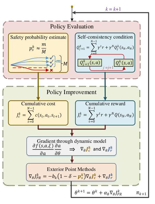
The chance constrained RL problem (2) is solved by iteratively updating $\pi_{k}$ and $b_{k}$ as shown in Fig. 1. However, in practice, the cost of solving $\pi_{k}$ in every iteration until convergence is computationally prohibitive, and an alternative is to replace the maximization by a gradient ascent step

where $\alpha_{\theta}>0$ is the learning rate of policy and the policy gradient $\nabla_{\theta}J_{EP}$ is derived as

In order to compute the above gradient, we have to obtain the current safe probability $p_{s}$ and its gradient $\nabla_{\theta}p_{s}$. Thanks to the available model, the safe probability $p_{s}$ can be easily estimated by sampling large numbers of trajectories. Specifically, we rollout $M$ trajectories with policy $\pi$. Suppose there are $m$ safe trajectories, then the safety probability is estimated by $p_{s}\approx\frac{m}{M}$. Note that this rollout procedure will not impose extra computation burden since these trajectories are also necessary for the update of actor-critic as we will discuss in III-B. Unfortunately, the gradient $\nabla_{\theta}p_{s}$ is still hard to obtain, which is also a key difficulty in solving the chance constrained problems. One possible solution is to find a substitute ascent direction to replace $\nabla_{\theta}p_{s}$. Inspired by the inequality $p_{s}\geq 1-J_{c}$ as shown in (5), a decreasing $J_{c}$ will push $p_{s}$ to the ascent direction, so we replace $\nabla_{\theta}p_{s}$ with $-\nabla_{\theta}J_{c}$. Consequently, the new proxy policy gradient becomes:

This policy gradient can be intuitively interpreted as follows. In order to solve the chance constrained problem (2), we simultaneously optimize the cumulative reward and the safe probability by gradient ascent. To balance the two objectives, the weight of $\nabla_{\theta}J_{c}$ is adaptively adjusted according to the current safe probability. We stress that CCAC is essentially different from previous methods which only constrain the lower bound. In CCAC, as long as the chance constraint $p_{s}\geq 1-\delta$ is satisfied, the weight of $\nabla_{\theta}J_{c}$ becomes zero and the safe probability will not be optimized. While previous methods keep optimizing $p_{s}$ until $J_{c}\leq\delta$, even when $p_{s}\geq 1-\delta$ is already satisfied. That is the underlying reason why CCAC is not conservative as previous methods. Finally, in practice, since the weight $b_{k}(1-\delta-p_{s})$ in (10) may become excessively large, we instead use the relative weights between $\nabla_{\theta}J_{r}$ and $\nabla_{\theta}J_{c}$.

The proposed algorithm CCAC is summarized in Algorithm 1 and Fig. 2.

In this subsection the main focus is on how to learn the policy and state-action values in the model-based actor-critic framework with parameterized functions. Importantly, the gradient of dynamic model will be utilized to attain an accurate ascent direction and thus improve the convergence rate [23, 24]. For an agent behaving according to policy $\pi$, the values of the state-action pair $(s,a)$ are defined as follows:

The expected cumulative reward $J_{r}$ can be expressed as a $N$-step form:

For large and continuous state spaces, both value function and policy are parameterized, as shown in (13). The parameterized state-action value function with parameter $w$ is usually named the “critic”, and the parameterized policy with parameter $\theta$ is named the “actor” [23].

The parameterized critic is trained by minimizing the average square error:

where $Q_{\text{target}}=\sum_{t=0}^{N-1}\gamma^{t}r\left(s_{t},a_{t}\right)+\gamma^{N}Q\left(s_{N},a_{N};w^{k}\right)$ is the $N$-step target. Note that the rollout length $N$ is equal to the horizon of chance constraint. The semi-gradient of the critic is

As discussed in III-A, the parameterized actor aims to maximize $J_{EP}$ via gradient ascent. The proxy gradient $\nabla_{\theta}J_{PR}$ is composed of $\nabla_{\theta}J_{r}$ and $\nabla_{\theta}J_{c}$, which are computed via backpropagation though time. Denoting $\frac{\partial s_{t}}{\partial\theta}$ as $\phi_{t}$, $\frac{\partial a_{t}}{\partial\theta}$ as $\psi_{t}$, then $\nabla_{\theta}J_{r}$ is derived as:

where

with $\phi_{0}=0$, and

The gradient $\nabla_{\theta}J_{c}$ can be derived similar to (16). Considering that $c\left(s,a,s^{\prime}\right)$ is an indicator function with zero gradient, it is replaced by the sigmoid function:

where $\eta>0$ is a scale factor. The benefits of calculating $\nabla_{\theta}J_{r}$ and $\nabla_{\theta}J_{c}$ in the model-based framework is that the gradients of first $N$ steps’ reward are computed analytically through the dynamic model. In contrast, model-free methods can not obtain these analytical gradients and thus only relies on the value function, which is usually inaccurate with high variance. In a word, the model-based framework achieves a faster convergence rate due to a more accurate gradient [24]. The convergence and optimality of model-based actor-critic framework have been well-studied in [25].

In this section the proposed CCAC is applied to a stochastic car-following scenario as shown in Fig. 3, where the ego car expects to drive closely with the front car to reduce wind drag, while keeping a minimum gap between the two cars. Concretely, the ego car and front car follow the kinematics model, where the front car is assumed to drive at a constant speed $v_{f}$ but its location $x_{f}^{\prime}$ is varying with uncertainty (e.g., due to the varying of road grade, wind drag). The minimum gap between the two cars is required to be kept at a high probability.

The discrete-time stochastic system is described by

The system state vector is $s=[v_{e}\quad v_{f}\quad\epsilon]^{\top}$ , where $v_{e}$ denotes the velocity of ego car, $v_{f}$ is the velocity of front car, and $\epsilon$ is the gap between the two cars. The action $a_{t}\in(-4,3)$ is the acceleration of ego car, and the disturbance $\xi_{t}\sim\mathcal{N}(0,1)$ is truncated in the interval $(-5,5)$. $T=0.1$ is the simulation time step. The chance constrained RL problem is defined as

where $v_{e,t}$ denotes the ego car velocity at time step $t$. In this setting, the agent is expected to drive fast and close to frontal car while keeping a minimum gap of 2m.

We implement CCAC algorithm on the problem above. Our parameterized actor and critic are both fully-connected neural networks. Each network has two hidden layers using rectified linear unit (ReLU) as activation functions, with 64 units per layer. The main hyper-parameters of the algorithm are listed in Table I. The penalty factor in (10) is set as $b_{k}=\text{min}(1000*1.01^{k},10000)$.

To demonstrate the advantages of CCAC, the performance is compared with model-free primal-dual method (MF-PD) [19], model-based fixed-weight penalty method (FWP), and two traditional safety techniques, i.e., stochastic model predictive control (SMPC) and safety shielding. The five methods are evaluated under two chance constraint thresholds 90.0% and 99.9%, i.e., $\delta=0.1$ and $\delta=0.001$. For FWP method, we test it with different penalty weights in advance and choose a large weight 20 for 99.9% threshold. Unfortunately, we find it is very hard to select an appropriate weight which produces a 90.0% safe policy. A small decline of the weight will cause a drastic decline of the safe probability. Therefore, we just choose a weight of 10 although it is relatively unsafe. For simplicity, FWP with weight 10 and 20 are shortly labeled as FWP-10 and FWP-20, respectively. The SMPC method adopts the stochastic tube approach to find the feasible actions under uncertainty [26]. The safety shielding method projects the action produced by an unconstrained policy network into the safe action region by solving a constrained optimization problems [27]. To handle the joint chance constraint, Boole’s inequality is also used in both SMPC and shielding.

We will analyse the five methods from the aspects of convergence rate, asymptotic performance and computation time.

References

- [1] V. Mnih, K. Kavukcuoglu, D. Silver, A. A. Rusu, J. Veness, and M. G. B. et al., “Human-level control through deep reinforcement learning,” Nature, vol. 518, pp. 529–533, 2015.
- [2] O. Vinyals, I. Babuschkin, W. Czarnecki, M. Mathieu, A. Dudzik, and J. C. et al., “Grandmaster level in starcraft ii using multi-agent reinforcement learning,” Nature, pp. 1–5, 2019.
- [3] D. Silver, J. Schrittwieser, K. Simonyan, I. Antonoglou, A. Huang, and A. G. et al., “Mastering the game of go without human knowledge,” Nature, vol. 550, pp. 354–359, 2017.
- [4] S. E. Li, X. Hu, K. Li, and C. Ahn, “Mechanism of vehicular periodic operation for optimal fuel economy in free-driving scenarios,” Iet Intelligent Transport Systems, vol. 9, pp. 306–313, 2015.
- [5] J. Garcıa and F. Fernández, “A comprehensive survey on safe reinforcement learning,” Journal of Machine Learning Research, vol. 16, no. 1, pp. 1437–1480, 2015.
- [6] G. Dulac-Arnold, D. J. Mankowitz, and T. Hester, “Challenges of real-world reinforcement learning,” ArXiv, vol. abs/1904.12901, 2019.
- [7] A. Tamar and S. Mannor, “Variance adjusted actor critic algorithms,” ArXiv, vol. abs/1310.3697, 2013.
- [8] Y. Chow, M. Ghavamzadeh, L. Janson, and M. Pavone, “Risk-constrained reinforcement learning with percentile risk criteria,” The Journal of Machine Learning Research, vol. 18, no. 1, pp. 6070–6120, 2017.
- [9] J. Achiam, D. Held, A. Tamar, and P. Abbeel, “Constrained policy optimization,” in International Conference on Machine Learning, pp. 22–31, PMLR, 2017.
- [10] C. Tessler, D. J. Mankowitz, and S. Mannor, “Reward constrained policy optimization,” in International Conference on Learning Representations, 2018.
- [11] T.-Y. Yang, J. Rosca, K. Narasimhan, and P. J. Ramadge, “Projection-based constrained policy optimization,” in International Conference on Learning Representations, 2019.
- [12] P. Geibel and F. Wysotzki, “Risk-sensitive reinforcement learning applied to control under constraints,” Journal of Artificial Intelligence Research, vol. 24, pp. 81–108, 2005.
- [13] D. Q. Mayne, J. B. Rawlings, C. V. Rao, and P. O. Scokaert, “Constrained model predictive control: Stability and optimality,” Automatica, vol. 36, no. 6, pp. 789–814, 2000.
- [14] J. Duan, S. E. Li, Y. Guan, Q. Sun, and B. Cheng, “Hierarchical reinforcement learning for self-driving decision-making without reliance on labelled driving data,” IET Intelligent Transport Systems, vol. 14, no. 5, pp. 297–305, 2020.
- [15] J. Duan, S. E. Li, Y. Guan, Q. Sun, and B. Cheng, “Hierarchical reinforcement learning for self-driving decision-making without reliance on labeled driving data,” ArXiv, vol. abs/2001.09816, 2020.
- [16] Y. Guan, Y. Ren, S. Li, Q. Sun, L. Luo, and K. Li, “Centralized cooperation for connected and automated vehicles at intersections by proximal policy optimization,” IEEE Transactions on Vehicular Technology, vol. 69, pp. 12597–12608, 2020.
- [17] M. Ono, M. Pavone, Y. Kuwata, and J. Balaram, “Chance-constrained dynamic programming with application to risk-aware robotic space exploration,” Autonomous Robots, vol. 39, pp. 555–571, 2015.
- [18] S. Paternain, M. Calvo-Fullana, L. F. O. Chamon, and A. Ribeiro, “Learning safe policies via primal-dual methods,” 2019 IEEE 58th Conference on Decision and Control (CDC), pp. 6491–6497, 2019.
- [19] S. Paternain, M. Calvo-Fullana, L. F. O. Chamon, and A. Ribeiro, “Safe policies for reinforcement learning via primal-dual methods,” ArXiv, vol. abs/1911.09101, 2019.
- [20] A. Mesbah, “Stochastic model predictive control: An overview and perspectives for future research,” IEEE Control Systems, vol. 36, pp. 30–44, 2016.
- [21] D. Bertsimas, D. B. Brown, and C. Caramanis, “Theory and applications of robust optimization,” SIAM review, vol. 53, no. 3, pp. 464–501, 2011.
- [22] S. P. Boyd and L. Vandenberghe, “Convex optimization,” IEEE Transactions on Automatic Control, vol. 51, pp. 1859–1859, 2006.
- [23] S. E. Li, “Reinforcement Learning and Control.” Tsinghua University: Lecture Notes. http://www.idlab-tsinghua.com/thulab/labweb/publications.html, 2020.
- [24] M. Deisenroth and C. E. Rasmussen, “PILCO: A model-based and data-efficient approach to policy search,” in Proceedings of the 28th International Conference on machine learning (ICML-11), pp. 465–472, Citeseer, 2011.
- [25] D. Liu, Q. Wei, D. Wang, X. Yang, and H. Li, Adaptive dynamic programming with applications in optimal control. Springer, 2017.
- [26] T. A. N. Heirung, J. Paulson, J. O’Leary, and A. Mesbah, “Stochastic model predictive control - how does it work?,” Computers & Chemical Engineering, vol. 114, pp. 158–170, 2018.
- [27] G. Dalal, K. Dvijotham, M. Vecerik, T. Hester, C. Paduraru, and Y. Tassa, “Safe exploration in continuous action spaces,” arXiv preprint arXiv:1801.08757, 2018.
- [28] A. Wächter and L. T. Biegler, “On the implementation of an interior-point filter line-search algorithm for large-scale nonlinear programming,” Mathematical Programming, vol. 106, pp. 25–57, 2006.