High-Dimensional Spatial Quantile Function-on-Scalar Regression

Zhengwu Zhang Xiao Wang Linglong Kong Hongtu Zhu

Abstract

This paper develops a novel spatial quantile function-on-scalar regression model, which studies the conditional spatial distribution of a high-dimensional functional response given scalar predictors. With the strength of both quantile regression and copula modeling, we are able to explicitly characterize the conditional distribution of the functional or image response on the whole spatial domain. Our method provides a comprehensive understanding of the effect of scalar covariates on functional responses across different quantile levels and also gives a practical way to generate new images for given covariate values. Theoretically, we establish the minimax rates of convergence for estimating coefficient functions under both fixed and random designs. We further develop an efficient primal-dual algorithm to handle high-dimensional image data. Simulations and real data analysis are conducted to examine the finite-sample performance.

Keywords: Copula; Function-on-scalar regression; Image analysis; Minimax rate of convergence; Quantile regression; Regularization; Reproducing kernel Hilbert space.

^†^† Zhengwu Zhang is Assistant Professor of Biostatistics, Department of Biostatistics and Computational Biology, University of Rochester, Rochester, New York 14627. Xiao Wang is Professor of Statistics, Department of Statistics, Purdue University, West Lafayette, IN 47907. Linglong Kong is Associate Professor of Statistics, Department of Mathematical and Statistical Sciences, University of Alberta, Edmonton, AB Canada T6G 2G1. Hongtu Zhu is Professor of Biostatistics, Department of Biostatistics, University of North Carolina, Chapel Hill, NC 27599.

1 Introduction

Functional data analysis (FDA) has been an active area of research in the past decade. Well-known monographs in this area include Ramsay and Silverman 2005, Ramsay and Silverman 2007, Bowman 2010 and Ferraty and Vieu 2006. Functional regression, particularly the functional linear regression model (FLM), has been extensively studied. Functional data can be treated as either response variables or covariate predictors (Greven and Scheipl 2017). In FLM, the mean dependence is modeled through a linear model generalizing the standard multiple linear regression model. The literature on FLM is vast. For example, scalar-on-function regression (a continuous response variable regressed on functional covariates) has been studied by Cai and Hall 2006, Crambes et al. 2009, Yuan et al. 2010, Hall and Horowitz 2007 and Wang et al. 2017. Function-on-function regression (a functional response regressed on functional predictors) has been investigated by Yao et al. 2005, Ramsay and Silverman 2005, Ivanescu et al. 2015, and Sun et al. 2018. Function-on-scalar regression (a functional response regressed on scalar predictors) has been studied by Ramsay and Silverman (Ramsay and Silverman 2005, Ch13, 2005), Reiss et al. 2010 and Goldsmith and Kitago 2016. The aim of this paper is to develop a spatial quantile function-on-scalar regression model and investigate its related computational and theoretical issues.

Different from the ordinary regression that only models conditional mean dependence, quantile regression as a more comprehensive procedure estimates conditional quantiles of the response variable. Since Koenker and Bassett Jr 1978, quantile regression has been an emerging field of statistical research and has been widely applied in many disciplines including neuroimaging, finance, and economics. Quantile regression is attractive because it estimates conditional quantiles and allows statistical inference on the response’s entire conditional distribution. Most importantly, quantile regression does not require a specified error distribution, providing a flexible framework for modeling complex non-Gaussian data. To date, while many studies have examined different quantile regression models, a limited number of these consider functional data. Cai and Xu 2008 studied quantile regression methods for a set of smooth coefficient time series models. Koenker 2004 and Yi and He 2009 developed quantile regression methods for longitudinal data. Wang et al. 2009 studied semi-parametric quantile auto-regression models in partially linear varying coefficient models using splines. Li et al. 2007 proposed a kernel quantile regression to estimate conditional quantile functions given training scalar covariates and responses. Kato et al. 2012 studied functional quantile regression with functional covariates and a scalar response.

In this paper, motivated by medical imaging analysis, we propose a novel spatial quantile function-on-scalar regression model (denoted by SQR) that studies the conditional spatial distribution of a functional response given scalar predictors. We are particularly interested in the case where the responses are high-dimensional functions or images obtained from $n$ independent subjects. Let the functional response be $\{Y(s):s\in{\cal S}\}$ on a field ${\cal S}$ and the scalar predictors be ${\bf x}\in\mathbb{R}^{p}$ . Our SQR model includes two major components. The first component is to model the marginal conditional distribution of $Y(s)$ given ${\bf x}$ at a fixed location $s$ . This task can be achieved by assuming that the $\tau$ -level conditional quantile of $Y(s)$ is assumed to be a linear function of ${\bf x}$ such that $Q_{Y(s)}(\tau|x)={\bf x}^{T}\boldsymbol{\beta}_{\tau}(s)$ , where $Q_{Y(s)}(\cdot|{\bf x})$ is the conditional quantile function of $Y(s)$ given ${\bf x}$ at a location $s$ and $\boldsymbol{\beta}_{\tau}(s)=(\beta_{\tau 1}(s),...,\beta_{\tau p}(s))^{T}$ contains $p$ unknown coefficient functions. The second component is to model the joint conditional distribution of $Y(s)$ among spatial locations via a copula model. We adopt a parametric copula to specify the joint distribution of $F_{(s,\bf x)}(Y(s))$ , where $F_{(s,\bf x)}(\cdot)$ is the conditional cumulative distribution function (CDF) of $Y(s)$ given ${\bf x}$ at $s$ and $F_{(s,\bf x)}(Y(s))$ follows a uniform distribution marginally. With these two components, we are able to explicitly characterize the conditional joint distribution of $Y(s)$ on the whole spatial domain ${\cal S}$ , forming a generative model that given $\bf x$ , we can simulate the image data $Y$ . The proposed method provides a framework to comprehensively understand the effects of scalar covariates (e.g., age, gender and disease status) on an image response, and a practical way to generate new images given covariates.

Although SQR has been studied in the literature (Reich et al. 2011; Reich 2012; Yang and He 2015; Su and Yang 2007; Kostov 2009; Hallin et al. 2009; Lu et al. 2014), our method differs from them in several important aspects. First, our SQR is primarily developed for handling large-scale image data $Y(s)$ with dense grids across multiple subjects. In contrast, most existing works on SQR focus on the development of statistical methods for analyzing simple spatial or longitudinal data (Reich et al. 2011; Reich 2012; Yang and He 2015; Hallin et al. 2009). For instance, Hallin et al. 2009 considered SQR for a strictly stationary real random field and proposed a local linear estimator of spatial quantile function. Second, we employ a parametric copula model to directly delineate the spatial dependence of image data within each subject. In contrast, most existing copula models were applied to quantile regression for different purposes and data types (Chen et al. 2009; Bouyé and Salmon 2013; Kraus and Czado 2017; De Backer et al. 2017; Wang et al. 2019). For instance, in Wang et al. 2019, the copula was used to model the temporal dependence of longitudinal data, while it is assumed a linear quantile regression model with $Q_{Y(t)}(\tau|{\bf x})={\bf x}^{T}\boldsymbol{\beta}_{0}(\tau)$ at a fixed time point $t$ and for given covariates ${\bf x}$ . However, our model assumes that the components of $\boldsymbol{\beta}_{\tau}(s)$ are functions of both $\tau$ and the spatial location. Third, the unknown coefficient functions $\boldsymbol{\beta}_{\tau}(s)$ are assumed to reside in a reproducing kernel Hilbert space and estimate them through minimizing a quantile check function (Koenker and Bassett Jr 1978) plus a roughness penalty. Furthermore, we estimate the unknown parameters of the copula model by using generalized least squares (Cressie 1985; Genton 1998). Most of the aforementioned papers involving coefficient function estimation utilize a finite-dimensional approximation, such as Fourier basis or through a roughness penalty, to regularize model complexity. It often leads to reasonable functional estimate, but at a price of complicating theoretical investigation.

Our main contributions are summarized as follows. First, it allows us to establish a Representation Theorem stating that, although the optimization is defined on an infinite-dimensional function space, its solution actually resides in a data-adaptive finite-dimensional subspace. This result guarantees an exact solution when optimization is carried out on this finite dimensional subspace. Second, we develop and implement an efficient primal-dual algorithm to handle large image data efficiently, as computation is generally very challenging with complex, high-dimensional images in quantile regression. We use extensive numerical studies to demonstrate the computational advantages of our method over other popular quantile regression optimization solvers such as the alternating direction method of multipliers (ADMM) algorithm (Boyd et al. 2011). Third, an important theoretical result of our work establishes the optimal convergence rate of the error in estimating these coefficient functions under both fixed and random designs. This generalizes the results in Cai and Yuan 2012 and Du and Wang 2014 for functional linear regression with a scalar response to the functional response scenario.

The rest of this paper is organized as follows. In Section 2, we introduce the mathematical details of the proposed SQR model, including the quantile regression and copula models. Section 3 introduces an efficient primal-dual algorithm to solve the high-dimensional quantile regression model and a generalized least square method to estimate parameters in the copula model. In Section 4, we studied the optimal convergence rate of the error in estimating the coefficient functions under both fixed and random designs. In Section 5, extensive numerical studies are used to illustrate the advantages of the proposed method.

2 Spatial Quantile Regression and Copula Models

The SQR model studies the conditional spatial distribution of an imaging response $\{Y(s):s\in{\cal S}\}$ given scalar predictors ${\bf x}\in\mathbb{R}^{p}$ . The conditional quantile function of $Y(s)$ given ${\bf x}$ for a fixed location $s$ at any quantile level $\tau\in(0,1)$ is assumed to be

Q_{Y(s)}(\tau|{\bf x})={\bf x}^{T}{\boldsymbol{\beta}}_{\tau}(s),

(2.1)

where ${\boldsymbol{\beta}}_{\tau}(s)=(\beta_{\tau 1}(s),\ldots,\beta_{\tau p}(s))^{T}\in{\cal F}^{p}$ is the vector of the unknown coefficient functions with each component of ${\boldsymbol{\beta}}_{\tau}$ residing in the function space ${\cal F}$ . Assume that ${\cal F}$ is a reproduce kernel Hilbert space (RKHS) ${\cal H}({K})$ with a reproducing kernel $K$ . Equation (2.1) completely specifies the conditional marginal distribution of $Y(s)$ given $\bf x$ and $s$ .

In practice, the image response is often observed at discrete locations $s_{1},\ldots,s_{m}$ in ${\cal S}$ , and the image values across different points in ${\cal S}$ are highly correlated. The conditional marginal distribution of $Y(s)$ is fully captured by (2.1), however, the spatial dependence among $Y(s)$ at different points in ${\cal S}$ is not modeled. To capture the joint distribution of $(Y(s_{1}),\ldots,Y(s_{m}))$ given scalar covariates $\bf x$ , we propose using copula models. Let the conditional CDF of $Y(s_{j})$ given $\bf x$ be $F_{(s_{j},{\bf x})}(y)=\mathbb{P}(Y(s_{j})\leq y|{\bf x})$ , $j=1,\ldots,m$ . The random variable $U_{\bf x}(s_{j})=F_{(s_{j},{\bf x})}(y)$ has a uniform marginal distribution. The conditional copula of $(Y(s_{1}),\ldots,Y(s_{m}))$ given ${\bf x}$ is defined as the conditional joint CDF of $(U_{\bf x}(s_{1}),\ldots,U_{\bf x}(s_{m}))$ given by

C_{{\boldsymbol{\theta}}}(u_{1},\ldots,u_{m})=\mathbb{P}\Big(U_{\bf x}(s_{1})\leq u_{1},\ldots,U_{\bf x}(s_{m})\leq u_{m}\Big|{\bf x}\Big).

(2.2)

The copula $C$ parameterized by ${\boldsymbol{\theta}}$ contains all information on the spatial dependence structure of $Y(\cdot)$ . In this paper, we adopt a parametric family of copulas $C_{{\boldsymbol{\theta}}}$ with ${\boldsymbol{\theta}}={\boldsymbol{\theta}}({\bf x})$ to characterize the joint conditional distribution of $(Y(s_{1}),\ldots,Y(s_{m}))$ . Therefore, the conditional joint distribution of $(Y(s_{1}),\ldots,Y(s_{m}))$ given ${\bf x}$ can be written as

\mathbb{P}\Big(Y(s_{1})\leq y_{1},\ldots,Y(s_{m})\leq y_{m}\Big|{\bf x}\Big)=C_{{\boldsymbol{\theta}}({\bf x})}\Big(F_{(s_{1},{\bf x})}(y_{1}),\ldots,F_{(s_{m},{\bf x})}(y_{m}))\Big).

There are many choices of copula models such as the Student-t copula (Demarta and McNeil 2005), the non-central $\chi^{2}$ -copula (Bárdossy 2006), and the Gaussian copula (Kazianka and Pilz 2010). It is a challenging task to determine the optimal choice of the copula. In our numerical analysis, we have examined 21 different copula models for the real diffusion tensor imaging (DTI) data set from the ADNI and found that the Student-t copula fits the data well in most of the times. Therefore, we adopt the Student-t copula in this paper, and denote it by

C_{\boldsymbol{\theta}}\Big(u_{1},\ldots,u_{m}\Big)={\boldsymbol{t}}_{\varrho,\boldsymbol{\Sigma}_{\boldsymbol{\theta}}}\Big(t_{\varrho}^{-1}(u_{1}),\ldots,t_{\varrho}^{-1}(u_{m})\Big),

where ${\boldsymbol{t}}_{\varrho,\boldsymbol{\Sigma}_{\boldsymbol{\theta}}}$ represents the multivariate t-distribution function with parameter $(\boldsymbol{\Sigma}_{\boldsymbol{\theta}},\varrho,{\bf 0})$ , and $t_{\varrho}^{-1}$ is the inverse CDF of t-distribution with $\varrho$ degrees of freedom. Note that $\varrho/(\varrho-2)\boldsymbol{\Sigma}_{\boldsymbol{\theta}}$ is the covariance matrix of the t-distribution for $\varrho>2$ in t-distribution. Furthermore, we use the Mateŕn family (Matérn 2013; Guttorp and Gneiting 2006) to specify a class of isotropic correlation functions given by

\mathrm{Corr}\Big(t_{\varrho}^{-1}(U(s+h)),t_{\varrho}^{-1}(U(s))~\Big|~{\bf x}\Big)=M(h)

that depends on the spatial separation parameter $h$ , where

M(h)={2^{1-\nu}\over\Gamma(\nu)}(\alpha\|h\|)^{\nu}K_{\nu}(\alpha\|h\|).

(2.3)

Here $K_{\nu}$ is the modified Bessel function of the second kind, $\nu>0$ is a smoothness parameter defining the smoothness of the sample path, and $\alpha>0$ is a spatial scale parameter. For our numerical studies, the parameters $\varrho$ and $\nu$ are selected and kept fixed, and the parameter $\alpha$ is treated as unknown. We assume that $\alpha$ depends on ${\bf x}$ . With an abuse of notation, we write the scale parameter as $\exp({\boldsymbol{\alpha}}^{T}{\bf x})$ , where ${\boldsymbol{\alpha}}\in\mathbb{R}^{p}$ .

Suppose that we observe $({\bf x}_{i},Y_{i}(s_{ij}))$ for subject $i$ and location $s_{ij}$ , $i=1,\ldots,n$ and $j=1,\ldots,m$ . In this paper, we consider two different designs for the location points $\{s_{ij}\}$ . The first one is called a fixed design, where the functional response are observed at the same locations across curves or images. That is, $s_{1j}=s_{2j}=\cdots=s_{nj}:=s_{j}$ for $j=1,\ldots,m$ . A second design, called random design, occurs when $\{s_{i1},\ldots,s_{im}\}$ are independently sampled from a distribution $\{\pi(s):s\in{\cal S}\}$ . Our goal is to estimate the coefficient functions $\beta_{\tau k}(\cdot)$ , $k=1,\ldots,p$ and the parameters in the copula model. There are two main challenges related to this problem. The first one is to construct statistically efficient estimates of unknown parameters, in particularly the infinite dimensional coefficient functions. The second one is to develop a numerically efficient algorithm to estimate unknown parameters to handle the high dimensionality of functional or image data.

3 Algorithms

3.1 Efficient Primal-Dual Algorithm for Estimating Coefficient Functions

For given observations $({\bf x}_{i},Y_{i}(s_{ij}))$ , we estimate the unknown parameters in the spatial quantile regression model (2.1) by solving the following optimization problem for a given $\tau\in(0,1)$ ,

\min_{{\boldsymbol{\beta}}\in{\cal F}^{p}}~~\sum_{i=1}^{n}\sum_{j=1}^{m}\rho_{\tau}(Y_{i}(s_{ij})-{\bf x}_{i}^{T}{\boldsymbol{\beta}}_{\tau}(s_{ij}))+{\lambda\over 2}\sum_{k=1}^{p}\mathcal{R}(\beta_{\tau k}),

(3.1)

where $\rho_{\tau}(r)=\tau rI(r>0)-(1-\tau)rI(r\leq 0)$ is the check function (Koenker and Bassett Jr 1978) and $I(\cdot)$ is the indicator function, ${\boldsymbol{\beta}}_{\tau}(s)=(\beta_{\tau 1}(s),\ldots,\beta_{\tau p}(s))^{T}$ are the coefficient functions, $\mathcal{R}$ is a roughness penalty on ${\boldsymbol{\beta}}_{\tau}$ , and $\lambda>0$ is a parameter controlling the smoothness penalty. We let $\mathcal{R}(\beta_{\tau k})=\|\beta_{\tau k}\|_{K}^{2}$ , where $\|\cdot\|_{K}$ is a semi-norm in the RKHS ${\cal H}(K)$ (Wahba 1990). For simplicity, we also assume that the null space of ${\cal H}(K)$ is $\{0\}$ . In the following derivations, we illustrate the algorithm in the case of fixed design, so that $Y(s_{ij})$ can be denoted as $Y(s_{j})$ . An extension to the case of a random design is straightforward.

Throughout the paper, Gaussian kernels are used for $K(\cdot,\cdot)$ just for simplicity. Other kernels can be easily incorporated. For example, some common options include the Laplace kernel $K(x,y)=\exp(-\sigma\|x-y\|_{1})$ , the polynomial kernel $K(x,y)=(\langle x,y\rangle+\sigma^{2})^{d}$ , and the inverse-quadratic kernel $K(x,y)=\sigma^{2}/(\sigma^{2}+\|x-y\|_{2}^{2})$ . Learning kernels is definitely a non-trivial question. A common way for learning kernels is to combine different kernels to improve them. For example, let $K(x,y)=c_{1}K_{1}(x,y)+c_{2}K_{2}(x,y)$ with $c_{1},c_{2}\geq 0$ , where $K_{1}$ and $K_{2}$ are potential kernels. The hyperparameters $c_{1}$ and $c_{2}$ can be set by cross-validation. Moreover, based on both simulations and real data analysis reported below, the use of Gaussian kernels leads to accurate estimation results.

Let $\widehat{\boldsymbol{\beta}}_{\tau}=(\widehat{\beta}_{\tau 1},\ldots,\widehat{\beta}_{\tau p})$ be the optimal solution of (3.1). For notational simplicity, we drop the subscript $\tau$ from the coefficient functions $\boldsymbol{\beta}$ when the context is clear. It is straightforward to establish a Representation Theorem (Wahba 1990) stating that $\widehat{\boldsymbol{\beta}}$ actually resides in a finite-dimensional subspace of ${\cal H}$ , which facilitates computation by reducing an infinite-dimensional optimization problem to a finite-dimensional one. Specifically,

\widehat{\beta}_{k}(s)=\mu_{k}+{\boldsymbol{b}}_{k}^{T}{\bf k}_{s},

(3.2)

for $k=1,\ldots,p$ , where $\mu_{k}$ is a scalar, ${\boldsymbol{b}}_{k}=(b_{k1},\ldots,b_{km})^{T}\in\mathbb{R}^{m}$ , and ${\bf k}_{s}=(K(s,s_{1}),\ldots,K(s,s_{m}))^{T}\in\mathbb{R}^{m}$ . The spatial smoothness of $\widehat{\beta}_{k}(s)$ comes from the RKHS assumption and the nature of image data. The use of regularization term $\lambda{\cal R}(\beta_{k})$ is to regularize the coefficients $\{b_{kj}\}_{j=1}^{m}$ to avoid overfitting and the use of GACV allows us to implicitly incorporate spatial correlations to select the tuning parameter $\lambda$ . Specifically, if there is high correlation among observations on the same subject, then GACV would lead to the selection of a large $\lambda$ .

The challenges of solving (3.1) under the parameterized form in (3.2) come from several aspects. First, the number of parameters to be estimated is generally large in medical imaging applications. In particular, each of the $p$ coefficient functions is represented by $m+1$ unknown parameters ( $m$ depends on the dimensionality of $Y$ ). For example, if $Y$ is a 2D image with a resolution of $50\times 50$ , we have $m=2500$ , and so we will need to estimate $p(2500+1)$ parameters. Second, the non-differentiability of the check function significantly increases the difficulty of the optimization problem. A straightforward optimization strategy for (3.1) is to use the popular ADMM algorithm (Boyd et al. 2011) that divides the optimization (3.1) into a few simpler optimization subproblems that can be solved iteratively. Details of the ADMM algorithm applied for solving (3.1) are included in the Supplement III. However, the convergence of ADMM can be very slow, and when the dimension of $Y$ is large, the computational cost of some subproblems of ADMM can be huge due to the large matrix inversion.

To overcome this computational challenge, we propose a primal-dual algorithm that converges much faster than ADMM and avoids large matrix inversion in each optimization iteration. The primal-dual kind of optimization approaches has been applied in the field of quantile regression. For instance, Koenker and Park 1996 described a primal-dual approach for computation of nonlinear quantile regression estimators based on the interior point method. Portnoy and Koenker 1997 and Portnoy 1997 compared the interior point method with existing simplex-based methods for quantile regression, and showed that the interior point approach was competitive and exhibited a rapidly increasing advantage for large problems. In our problem, to estimate coefficient function $\widehat{\beta}_{k}$ corresponding to the covariate ${x}_{k}$ for $k=1,\ldots,p$ , we rely on the formula (3.2). However, the traditional interior point algorithm for quantile regression (Koenker and Park 1996; Portnoy and Koenker 1997; Portnoy 1997) does not involve $\{{\bf b}_{k}\}$ that are difficult to solve.

We make a critical observation that the primal variable ${\bf\mu}=(\mu_{1},\ldots,\mu_{p})^{T}$ is also a dual variable for the dual problem, which leads to the following efficient optimization strategy. Similar to Li et al. 2007, we introduce positive residuals $\{\xi_{ij}\in\mathbb{R}_{+}\}$ and negative residuals $\{\zeta_{ij}\in\mathbb{R}_{+}\}$ such that $-\zeta_{ij}\leq Y_{i}(s_{j})-\widehat{Y}_{i}({s_{j}})\leq\xi_{ij}$ , where $\widehat{Y}_{i}(s_{j})={\bf x}_{i}^{T}\widehat{{\boldsymbol{\beta}}}(s_{j})$ . We obtain an optimization problem that is equivalent to (3.1) as follows:

	$\displaystyle\min_{{\boldsymbol{\xi}},{\boldsymbol{\zeta}},{\boldsymbol{\mu}},{\boldsymbol{b}}}$	$\displaystyle~~\tau\sum_{i=1}^{n}\sum_{j=1}^{m}\xi_{ij}+(1-\tau)\sum_{i=1}^{n}\sum_{j=1}^{m}\zeta_{ij}+{\lambda\over 2}\sum_{k=1}^{p}{\boldsymbol{b}}_{k}^{T}{\boldsymbol{\Sigma}}{\boldsymbol{b}}_{k}$
	$\displaystyle s.t.$	$\displaystyle~~Y_{i}(s_{j})={\bf x}_{i}^{T}{\boldsymbol{\mu}}+\sum_{k=1}^{p}x_{ik}{\bf k}_{s_{j}}^{T}{\boldsymbol{b}}_{k}+\xi_{ij}-\zeta_{ij},~i=1,\ldots,n,~j=1,\ldots,m,~({\boldsymbol{\xi}},{\boldsymbol{\zeta}})\in\mathbb{R}_{+}^{nm},$

where ${\boldsymbol{\Sigma}}=(K(s_{i},s_{j}))\in\mathbb{R}^{m\times m}$ , ${\boldsymbol{\mu}}=(\mu_{1},\ldots,\mu_{p})^{T}\in\mathbb{R}^{p}$ , $x_{ik}$ is the $k$ -th element of ${\bf x}_{i}$ , and $\xi_{ij}$ and $\zeta_{ij}$ are elements of ${\boldsymbol{\xi}}$ and ${\boldsymbol{\zeta}}$ , respectively. The primal Lagrangian function is defined as

	$\displaystyle\Lambda$	$\displaystyle=\tau\sum_{i=1}^{n}\sum_{j=1}^{m}\xi_{ij}+(1-\tau)\sum_{i=1}^{n}\sum_{j=1}^{m}\zeta_{ij}+{\lambda\over 2}\sum_{k=1}^{p}{\boldsymbol{b}}_{k}^{T}{\boldsymbol{\Sigma}}{\boldsymbol{b}}_{k}$
		$\displaystyle-\sum_{i=1}^{n}\sum_{j=1}^{m}d_{ij}({\bf x}_{i}^{T}{\boldsymbol{\mu}}+\sum_{k=1}^{p}x_{ik}{\bf k}_{s_{j}}^{T}{\boldsymbol{b}}_{k}+\xi_{ij}-\zeta_{ij}-Y_{i}(s_{j}))-\sum_{i=1}^{n}\sum_{j=1}^{m}\kappa_{ij}\xi_{ij}-\sum_{i=1}^{n}\sum_{j=1}^{m}\tilde{\kappa}_{ij}\zeta_{ij},$

where $d_{ij},\kappa_{ij}\geq 0,$ and $\tilde{\kappa}_{ij}\geq 0$ are Lagrange multipliers. Setting the derivatives of $\Lambda$ to zero leads to

$\displaystyle{\partial\over\partial{\boldsymbol{\mu}}}:$	$\displaystyle~~~\sum_{i=1}^{n}\sum_{j=1}^{m}d_{ij}{\bf x}_{i}={\bf 0},$	(3.3)
$\displaystyle{\partial\over\partial{\boldsymbol{b}}_{k}}:$	$\displaystyle~~~{\boldsymbol{b}}_{k}={1\over\lambda}\sum_{i=1}^{n}\sum_{j=1}^{m}d_{ij}x_{ik}{\boldsymbol{\Sigma}}^{-1}{\bf k}_{s_{j}},$	(3.4)
$\displaystyle{\partial\over\partial\xi_{ij}}:$	$\displaystyle~~~d_{ij}=\tau-\kappa_{ij}$	(3.5)
$\displaystyle{\partial\over\partial\zeta_{ij}}:$	$\displaystyle~~~d_{ij}=-(1-\tau)+\tilde{\kappa}_{ij},$	(3.6)

and the Karush-Kuhn-Tucker conditions are

$\displaystyle d_{ij}({\bf x}_{i}^{T}{\boldsymbol{\mu}}+\sum_{k=1}^{p}x_{ik}{\bf k}_{s_{j}}^{T}{\boldsymbol{b}}_{k}+\xi_{ij}-\zeta_{ij}-Y_{i}(s_{j}))=$	$\displaystyle 0,$	(3.7)
$\displaystyle\kappa_{ij}\xi_{ij}=$	$\displaystyle 0,$	(3.8)
$\displaystyle\tilde{\kappa}_{ij}\zeta_{ij}=$	$\displaystyle 0.$	(3.9)

Since $\kappa_{ij}$ and $\tilde{\kappa}_{ij}$ must be non-negative, following (3.5) and (3.6), we have $d_{ij}\in[-(1-\tau),\tau]$ . Furthermore, we have

d_{ij}\in(-(1-\tau),\tau)\Rightarrow\kappa_{ij},\tilde{\kappa}_{ij}>0\Rightarrow\xi_{ij}=\zeta_{ij}=0\Rightarrow Y_{i}(s_{j})={\bf x}_{i}^{T}{\boldsymbol{\mu}}+\sum_{k=1}^{p}x_{ik}{\bf k}_{s_{j}}^{T}{\boldsymbol{b}}_{k}.

Define $Se$ as the index set

Se=\{(i,j):d_{ij}\in(-(1-\tau),\tau),i=1,\ldots,n,~j=1,\ldots,m\}.

If $(i,j)\in Se$ , we have

\displaystyle Y_{i}(s_{j})

\displaystyle={\bf x}_{i}^{T}{\boldsymbol{\mu}}+\sum_{k=1}^{p}x_{ik}{\bf k}_{s_{j}}^{T}{\boldsymbol{b}}_{k}={\bf x}_{i}^{T}{\boldsymbol{\mu}}+{1\over\lambda}\sum_{i^{\prime}=1}^{n}\sum_{j^{\prime}=1}^{m}d_{i^{\prime}j^{\prime}}{\bf x}_{i^{\prime}}^{T}{\bf x}_{i}K(s_{j^{\prime}},s_{j}).

(3.10)

If the $\{d_{ij}\}$ are known, then we may solve (3.1) by obtaining $\boldsymbol{\mu}$ and ${\boldsymbol{b}}_{k}$ through (3.10) and (3.4). However, it is difficult to obtain $d_{ij}$ in the presence of linear constraints (3.3).

Next, we consider the Lagrange dual problem where the dual function is defined as $\inf_{{\boldsymbol{\xi}},{\boldsymbol{\zeta}},{\boldsymbol{\kappa}},\tilde{\boldsymbol{\kappa}}}\Lambda$ . To simplify the notation, we vectorize our data by letting ${\bf y}=(Y_{i}(s_{j}))\in\mathbb{R}^{nm}$ , ${\boldsymbol{d}}=(d_{ij})\in\mathbb{R}^{nm}$ , and ${\bf X}=[{\bf x}_{1};...;{\bf x}_{n}]\in\mathbb{R}^{p\times n}$ . With these notations, from (3.3)-(3.6), the dual problem can be written as

	$\displaystyle\max_{\boldsymbol{d}}$	$\displaystyle~~-{1\over 2\lambda}{\boldsymbol{d}}^{T}{\bf Q}{\boldsymbol{d}}+{\boldsymbol{d}}^{T}{\bf y},$		(3.11)
	$\displaystyle s.t.$	$\displaystyle~~{\boldsymbol{d}}\in[-(1-\tau),\tau]^{nm},~~\widetilde{\bf X}{\boldsymbol{d}}={\bf 0},$

where ${\bf Q}={\boldsymbol{\Sigma}}\otimes{\bf X}^{T}{\bf X}\in\mathbb{R}^{nm\times nm}$ and $\widetilde{\bf X}=(e\otimes{\bf X}^{T})^{T}\in\mathbb{R}^{p\times nm}$ with $e=[1,..,1]^{T}\in\mathbb{R}^{m}$ and $\otimes$ indicating the Kronecker product . The optimization problem (3.11) is a high-dimensional quadratic programming problem with both box and linear constraints. Because of the linear constraints, we may not be able to solve this problem efficiently. However, these linear constraints can be removed using the primal information because the primal variable $\boldsymbol{\mu}$ is also a dual variable for the dual problem. Hence, if $\boldsymbol{\mu}$ is known, the dual variable $\boldsymbol{d}$ can be obtained by solving

	$\displaystyle\max_{\boldsymbol{d}}$	$\displaystyle~~-{1\over 2\lambda}{\boldsymbol{d}}^{T}{\bf Q}{\boldsymbol{d}}+{\boldsymbol{d}}^{T}({\bf y}-\widetilde{\bf X}^{T}{\boldsymbol{\mu}}),$		(3.12)
	$\displaystyle s.t$	$\displaystyle~~{\boldsymbol{d}}\in[-(1-\tau),\tau]^{nm}$

The quadratic program (3.12) with the box constraints can be solved efficiently with the algorithm introduced in De Angelis et al. 1997. Therefore, our optimization strategy for (3.1) is to solve the primal and dual problems alternatively until convergence.

Next, we discuss the effective degrees of freedom of our model and smoothing parameter selection. The divergence

\mbox{div}(\widehat{Y})=\sum_{i=1}^{n}\sum_{j=1}^{m}{\partial\widehat{Y}_{i}(s_{j})\over\partial Y_{i}(s_{j})}

has been used by many authors (Efron 1986; Meyer and Woodroofe 2000; Koenker 2005; Li et al. 2007) to estimate the effective dimension for a general modeling procedure. This idea arises from the framework of Stein’s unbiased risk estimation theory (Stein 1981). Under the setting of nonparametric regression with homoscedastic normal errors, divergence is an unbiased estimate of the sum of the covariance between individual fitted values and the corresponding observed values. Koenker et al. 1994 heuristically argued that, under the one-dimensional nonparametric quantile smoothing spline model, the number of interpolated observations is a plausible estimate for the effective dimension of the fitted model. Li et al. 2007 proved that, under the one-dimensional nonparametric kernel quantile regression model, the divergence is exactly equal to the number of interpolated observations. In this paper, we formally prove that the divergence is exactly the same as the the number of interpolated $Y_{i}(s_{j})$ ’s, thus justifying its use for the selection of $\lambda$ .

Theorem 3.1

Let $Se=\{(i,j):Y_{i}(s_{j})=\widehat{Y}_{i}(s_{j})\}$ . For any fixed $\lambda>0$ and any $Y_{i}(s_{j})$ , we have

\mbox{div}(\widehat{Y})=|{Se}|.

The proof is presented in the Appendix. The choice of the smoothing parameter $\lambda$ is a critical but difficult question. Commonly used criteria for quantile regression include the Schwarz information criterion (SIC) (Schwarz 1978; Koenker et al. 1994) and the generalized approximate cross validation (GACV) (Yuan 2006). We adopt the GACV criteria in this paper to select $\lambda$ :

\mbox{GACV}(\lambda)={\sum_{i=1}^{n}\sum_{j=1}^{m}\rho_{\tau}(Y_{i}(s_{j})-{\bf x}_{i}^{T}\widehat{\boldsymbol{\beta}}(s_{j}))\over nm-df},

(3.13)

where $df$ is a measure of the effective dimensionality of the fitted model that can be unbiasedly estimated by the divergence as defined in Theorem 3.1.

3.2 Generalized Least Squares for the Copula

The quantile regression model in (2.1) only gives the marginal distribution of $Y(s_{j})$ given $\bf x$ . To obtain the joint distribution of $(Y(s_{1}),\ldots,Y(s_{m}))$ given $\bf x$ , we utilize the copula model. Let $U_{\bf x}(s_{j})=F_{(s_{j},{\bf x})}(Y(s_{j}))$ , $j=1,\ldots,m$ . We characterize the joint distribution of $(U_{\bf x}(s_{1}),\ldots,U_{\bf x}(s_{m}))$ using the Student-t copula model

C_{\boldsymbol{\theta}}\Big(u_{1},\ldots,u_{m}\Big|{\bf x}\Big)=\mathbb{P}\Big(U_{\bf x}(s_{1})<u_{1},\ldots,U_{\bf x}(s_{m})<u_{m}\Big|{\bf x}\Big)={\boldsymbol{t}}_{\varrho,{\boldsymbol{\Sigma}}_{{\boldsymbol{\theta}}({\bf x})}}\Big(t_{\varrho}^{-1}(u_{1}),\ldots,t_{\varrho}^{-1}(u_{m})\Big).

The covariance function follows the Mateŕn model (Matérn 2013; Guttorp and Gneiting 2006), which specifies a class of isotropic correlation functions

\mathrm{Corr}(t_{\varrho}^{-1}(U(s_{j})),t_{\varrho}^{-1}(U(s_{k}))|{\bf x})=M(s_{j}-s_{k}),~~~s_{j}\neq s_{k}.

For the Mateŕn model, we can easily verify that

\displaystyle\mathrm{Var}\Big(t_{\varrho}^{-1}(U(s_{j}))-t_{\varrho}^{-1}(U(s_{k}))\Big)=2\varrho/(\varrho-2)(1-M(h)),

where $h=s_{j}-s_{k}$ . We denote $N(h)=\{(s_{j},s_{k}):s_{j}-s_{k}=h;j,k=1,\ldots,m\}$ to be the set of all pairs of locations having lag difference $h$ . Denote $\gamma(h)=1-M(h)$ . Matheron 1963 defined the earliest unbiased nonparametric variogram estimator of $\gamma(h)$ for a fixed lag $h$ as

2\widehat{\gamma}(h)={\varrho-2\over\varrho|N(h)|}\sum_{(s_{j},s_{k})\in N(h)}\Big|t_{\varrho}^{-1}(U(s_{j}))-t_{\varrho}^{-1}(U(s_{k}))\Big|^{2}.

The method of generalized least squares determines an estimator $\widehat{\boldsymbol{\theta}}$ by minimizing

G({\boldsymbol{\theta}})=(2\widehat{\gamma}-2\gamma({\boldsymbol{\theta}}))^{T}\Omega^{-1}(2\widehat{\gamma}-2\gamma({\boldsymbol{\theta}})).

Cressie 1985 studied the method of generalized least squares for variogram fitting in the case where the variance-covariance matrix $\Omega$ is diagonal, leading to the method of weighted least squares (WLS). Genton 1998 discussed a more general framework to approximate the variance-covariance matrix and significantly improved the fit. We first discuss how to construct pseudo copula observations. Pseudo copula observations $\tilde{U}_{{\bf x}_{i}}(s_{j})$ can be constructed as $\widehat{F}_{(s_{j},\bf x)}(Y_{i}(s_{j}))$ , for $i=1,\ldots,n$ , $j=1,\ldots,m$ , where $\widehat{F}_{j}$ is the estimated conditional CDF of $Y_{i}(s_{j})$ given ${\bf x}_{i}$ . The information contained in the dual problem is the key to obtain these pseudo copula observations. Let $\tilde{d}_{ij}={d}_{ij}+(1-\tau)$ such that $\tilde{d}_{ij}(\tau;{\bf x}_{j},s_{j}):[0,1]\rightarrow[0,1]$ . This ${\tilde{d}}_{ij}$ plays a crucial role in connecting the statistical theory of quantile regression to the classical theory of rank tests (Gutenbrunner and Jurecková 1992; Gutenbrunner et al. 1993). In particular, let $\widehat{Y}_{i}(s_{j})={\bf x}_{i}^{T}\widehat{\boldsymbol{\beta}}_{\tau}(s_{j})$ be the fitted value. We have

\tilde{d}(\tau;{\bf x}_{i},s_{j})=\left\{\begin{array}[]{ll}1&\mbox{if }~Y_{i}(s_{j})>\widehat{Y}_{i}(s_{j}),\\ (0,1)&\mbox{if }~Y_{i}(s_{j})=\widehat{Y}_{i}(s_{j}),\\ 0&\mbox{if }~Y_{i}(s_{j})<\widehat{Y}_{i}(s_{j}).\end{array}\right.

(3.14)

The integral $\int_{0}^{1}\tilde{d}(\tau;{\bf x}_{i},s_{j})d\tau$ provides a natural estimate of conditional quantile level of the observed response $Y_{i}(s_{j})$ given ${\bf x}_{i}$ , that is

\tilde{U}_{{\bf x}_{i}}(s_{j})=\int_{0}^{1}\tilde{d}(\tau;{\bf x}_{i},s_{j})d\tau,~~~i=1,\ldots,n~\mbox{and}~j=1,\ldots,m.

(3.15)

We denote different lags $h$ by $h_{k}$ for $k=1,\ldots,K$ , and let $g_{\bf x}(\boldsymbol{\theta})=(2\widehat{\gamma}_{\bf x}(h_{1})-2\gamma_{\bf x}(h_{1},\boldsymbol{\theta}),\ldots,2\widehat{\gamma}_{\bf x}(h_{K})-2\gamma_{\bf x}(h_{K},\boldsymbol{\theta}))^{T}$ . We utilize Genton’s method (Genton 1998) to estimate $\Omega$ in the generalized least squares. Let $V_{\bf x}(\boldsymbol{\theta})$ be the inverse of the dispersion matrix of the sample variogram $\mathbb{E}(g_{\bf x}({\boldsymbol{\theta}})g_{\bf x}({\boldsymbol{\theta}})^{T}|{\bf x})$ . We can obtain $\boldsymbol{\theta}$ via:

\widehat{\boldsymbol{\theta}}=\arg\min_{\boldsymbol{\theta}}\sum_{i=1}^{n}g_{{\bf x}_{i}}^{T}(\boldsymbol{\theta})V_{{\bf x}_{i}}(\boldsymbol{\theta})g_{{\bf x}_{i}}(\boldsymbol{\theta}).

(3.16)

The asymptotic properties of this estimator have been established in Cressie 1985; Cressie 2015 and Lahiri et al. 2002. We omit the details here.

4 Optimal Rate of Convergence

In this section, we establish the minimax rate of convergence of estimating the coefficient functions. We consider the two different designs introduced previously. For the fixed design, the spatial functional response is observed at the same locations across curves, that is, $m_{1}=m_{2}=\cdots=m_{n}:=m$ and $s_{1j}=s_{2j}=\cdots=s_{nj}:=s_{j}$ for $j=1,\ldots,m$ . Assume that, as $m\rightarrow\infty$ , the empirical distribution of $s_{j}$ ’s converges to a fixed distribution $\pi(s)$ . For the random design, the $s_{ij}$ are independently sampled from a distribution. With an abuse of notation, we also denote it by $\pi(s)$ . For any two $p$ -dimensional vector functions ${\boldsymbol{f}}_{1},{\boldsymbol{f}}_{2}\in{\cal F}^{p}$ , we define the $\mathbb{L}_{2}$ -distance as

\Big\|{\boldsymbol{f}}_{1}-{\boldsymbol{f}}_{2}\Big\|_{s,2}^{2}={\displaystyle\int_{\cal S}\sum_{k=1}^{p}(f_{1k}(s)-f_{2k}(s))^{2}\pi(s)ds}.

For any fixed quantile level $\tau\in(0,1)$ , let $\beta_{\tau k}$ be the true coefficient function. We measure the accuracy of the estimation of $\widehat{\beta}_{\tau k}$ by

{\cal E}_{\tau}(\widehat{\beta}_{\tau k},\beta_{\tau k})=\big\|\widehat{\beta}_{\tau k}-\beta_{\tau k}\big\|_{s,2}^{2}.

The rate of convergence of ${\cal E}_{\tau}(\widehat{\beta}_{\tau k},\beta_{\tau k})$ as the sample size $n$ and the location sampling frequency $m$ increase reflects the difficulty of the estimation problem.

4.1 Minimax lower bound

The following result establishes the minimax lower bound for estimating ${\boldsymbol{\beta}}_{\tau}$ over ${\cal F}^{p}$ under both fixed and random designs. The minimax lower bound is given in the following theorem.

Theorem 4.1

Fix $\tau\in(0,1)$ , and suppose the eigenvalues $\{\rho_{k}:k\geq 1\}$ of the reproducing kernel $K$ satisfies $\rho_{k}\asymp k^{-2r}$ for some constant $0<r<\infty$ . Then

(a).

for the fixed design,

\lim_{a_{\tau}\rightarrow 0}\lim_{n,m\rightarrow\infty}\inf_{\widetilde{\boldsymbol{\beta}}_{\tau}\in{\cal F}^{p}}\sup_{{\boldsymbol{\beta}}_{\tau}\in{\cal F}^{p}}\mathbb{P}\Big({\cal E}_{\tau}(\tilde{\boldsymbol{\beta}}_{\tau},{\boldsymbol{\beta}}_{\tau})\geq a_{\tau}(n^{-1}+m^{-2r})\Big)=1;

(4.1)

(b).

and for the random design,

\lim_{a_{\tau}\rightarrow 0}\lim_{n,m\rightarrow\infty}\inf_{\widetilde{\boldsymbol{\beta}}_{\tau}\in{\cal F}^{p}}\sup_{{\boldsymbol{\beta}}_{\tau}\in{\cal F}^{p}}\mathbb{P}\Big({\cal E}_{\tau}(\tilde{\boldsymbol{\beta}}_{\tau},{\boldsymbol{\beta}}_{\tau})\geq a_{\tau}((nm)^{-{2r\over 2r+1}}+n^{-1})\Big)=1.

(4.2)

The above infimums are taken over all possible estimators $\widetilde{\boldsymbol{\beta}}_{\tau}$ based on the training data.

Remark 4.1

The lower bounds established in Theorem 4.1 depend on the decay rate of the eigenvalues of the reproducing kernel $K$ . The lower bounds are different between the fixed design and the random design. For both designs, when the number of locations $m$ is large, it has no effect on the rate of convergence and the optimal rate is of order $n^{-1}$ . On the other hand, a phrase transition phenomenon happens when $m$ is of order $n^{1/2r}$ . If $m$ is below this order, the optimal rate for the fixed design is of order $m^{-2r}$ and for the random design is of order $(mn)^{-2r/(2r+1)}$ . We may conclude that the random design leads to a better result in terms of the rate of convergence. Similar phenomenon has been studied when estimating the mean of functional data (Cai and Yuan 2012).

Remark 4.2

The constants $a_{\tau}$ in (4.1) and (4.2) depend on the quantile level $\tau$ . If we assume $\tau\in{\cal T}\subset(0,1)$ with ${\cal T}$ being a compact subset of $(0,1)$ , it is possible to extend Theorem 4.1 to hold uniformly for all $\tau$ , that is, we may choose a constant $a$ in both (4.1) and (4.2) that does not depend on $\tau$ . This result can be established by a slight modification of the proof of Theorem 4.1.

4.2 Minimax upper bound

In this section, we consider the upper bound for the minimax risk and construct specific rate optimal estimators under both designs. The upper bound shows that the rates given in Theorem 4.1 are sharp. Specifically, we adopt the roughness regularization method to estimate the coefficient function vector ${\boldsymbol{\beta}}_{\tau}\in{\cal F}^{p}$ by minimizing

\sum_{i=1}^{n}\sum_{j=1}^{m}\rho_{\tau}\big(Y_{i}(s_{ij})-{\bf x}_{i}^{T}{\boldsymbol{\beta}}_{\tau}(s_{ij})\big)+\lambda\sum_{k=1}^{p}\|{\beta}_{\tau k}\|_{K}^{2},

(4.3)

where $\lambda>0$ is a tuning parameter balancing fidelity to the data and smoothness of the estimate. Let $\widehat{\boldsymbol{\beta}}_{\tau}$ be the estimate from (4.3).

We now introduce the following main assumptions, which put some constraints on the conditional CDF of $Y(s)$ given $\bf x$ and $s$ and the design matrix from the covariates:

A1.

Let the CDF of $Y(s)$ given $\bf x$ and $s$ be $F_{(s,\bf x)}(y)=\mathbb{P}(Y(s)\leq y|{\bf x})$ . Assume that there exist constants $c_{0}>0$ and $c_{1}>0$ such that for any $u$ satisfying $|u|\leq c_{0}$ , $\big|F_{(s,\bf x)}(u)-F_{(s,\bf x)}(0)\big|\geq c_{1}|u|^{2}$ .
A2.

Assume ${\bf x}$ belongs to a compact subset of $\mathbb{R}^{p}$ and that the eigenvalues of $\mathbb{E}({\bf x}{\bf x}^{T})$ are bounded below and above by some positive constants $c_{2}$ and $1/c_{2}$ , respectively.

Theorem 4.2

Fix $\tau\in(0,1)$ . Suppose the eigenvalues $\{\rho_{k}:k\geq 1\}$ of the reproducing kernel $K$ satisfies $\rho_{k}\asymp k^{-2r}$ for some constant $0<r<\infty$ . If A1 and A2 hold, then

(a).

for the fixed design,

\lim_{A_{\tau}\rightarrow\infty}\lim_{n,m\rightarrow\infty}\sup_{{\boldsymbol{\beta}}_{\tau}\in{\cal F}^{p}}\mathbb{P}\Big({\cal E}_{n}(\widehat{\boldsymbol{\beta}}_{\tau},{\boldsymbol{\beta}}_{\tau})\geq A_{\tau}(n^{-1}+m^{-2r})\Big)=0

(4.4)

for any $\lambda=O(nm(n^{-1}+m^{-2r}))$ ;

(b).

and for the random design,

\lim_{A_{\tau}\rightarrow\infty}\lim_{n,m\rightarrow\infty}\sup_{{\boldsymbol{\beta}}_{\tau}\in{\cal F}^{p}}\mathbb{P}\Big({\cal E}_{n}(\widehat{\boldsymbol{\beta}}_{\tau},{\boldsymbol{\beta}}_{\tau})\geq A_{\tau}((nm)^{-{2r\over 2r+1}}+n^{-1})\Big)=0

(4.5)

for any $\lambda=O(nm(n^{-1}+m^{-2r/(2r+1)}))$ .

Remark 4.3

Combining Theorems 4.1 and 4.2 demonstrates that $\widehat{\boldsymbol{\beta}}_{\lambda}$ is rate-optimal. Similar to Theorem 4.1, the rate of convergence shows both similarities and significant differences between fixed and random designs. In particular, for the random design, the optimal rate is $(mn)^{-2r/(2r+1)}$ when $m=O(n^{1/2r})$ and it is interesting to note that the dependency among $Y_{i}(s_{ij})$ does not affect the rate of convergence.

It is possible to extend Theorem 2 to hold uniformly for all $\tau$ in some domain of interest. In the following, we assume that $\tau\in{\cal T}$ , with ${\cal T}$ being a compact subset of $(0,1)$ .

Corollary 4.1

Assume $\tau\in{\cal T}$ , and assume the same conditions of Theorem 4.2.

(a).

For the fixed design, we have

\sup_{\tau\in{\cal T}}\big\|\widehat{\boldsymbol{\beta}}_{\tau}-{\boldsymbol{\beta}}_{\tau}\big\|_{s,2}^{2}=O_{p}\Big(n^{-1}+m^{-2r}\Big)

(4.6)

for any $\lambda=O(nm(n^{-1}+m^{-2r}))$ ;

(b).

For the random design, we have

\sup_{\tau\in{\cal T}}\big\|\widehat{\boldsymbol{\beta}}_{\tau}-{\boldsymbol{\beta}}_{\tau}\big\|_{s,2}^{2}=O_{p}\Big((nm)^{-{2r\over 2r+1}}+n^{-1})\Big)

(4.7)

for any $\lambda=O(nm(n^{-1}+m^{-2r/(2r+1)}))$ .

5 Numerical Analysis

In the following section, we evaluate the finite sample performance of our method by using both simulated and real data sets, and compare with other spatial quantile regression methods.

5.1 Algorithm Complexity

We first study the computational complexity of the proposed primal-dual algorithm for SQR. As a comparison, we developed another optimization algorithm based on the popular ADMM (Boyd et al. 2011). Please refer to Supplement III for more details on the ADMM algorithm. The iterative ADMM algorithm divides the optimization problem in (3.1) into multiple sub-problems, each of which has an explicit solution. In the high-dimensional scenario, however, explicitly solving each step is not computationally easy since it requires the multiplication and inversion of large matrices. Another disadvantage of using ADMM is its convergence rate, which can be poor when high accuracy is desired (Boyd et al. 2011). In contrast, the proposed primal-dual algorithm converges very quick and does not require matrix inversion. We implemented and compared both algorithms in MATLAB on a MacBook Pro with a 2.5 GHz Intel Core i7 CPU and 16 GB of RAM. In addition, an Bayesian spatial quantile regression (BSQR) method proposed in Reich et al. 2011 was implemented in R and compared with our method. In our implementation, $5000$ MCMC samples were drawn and the final results were summarized based on a burn-in of first $1000$ samples.

Simulation data sets were generated from the following model:

Y_{i}(s_{j})=x_{i1}\beta_{\tau 1}(s_{j})+x_{i2}\beta_{\tau 2}(s_{j})+x_{i3}\beta_{\tau 3}(s_{j})+\eta_{i}(s_{j},\tau),

for $i=1,\ldots,n;$ $j=1,\ldots,m,$ where $x_{i1}=1$ , $x_{i2}\sim Bernoulli(0.5)$ , $x_{i3}\sim Uniform(0,1)$ , and $\{s_{j}\}$ are evenly sampled on $[0,1]$ . We also set $\eta_{i}(s_{j})=v_{i}(s_{j})+\epsilon_{i}(s_{j})$ , where $\epsilon_{i}(s_{j})\sim N(0,0.1)$ , and $(v_{i}(s_{1}),\ldots,v_{i}(s_{m}))$ follows a multivariate normal distribution with zero mean and a covariance matrix taking the form $\mbox{Cov}(v_{i}(s_{j}),v_{i}(s_{l}))=a*\exp(-((s_{j}-s_{l})/h)^{2})$ with $a=0.6$ and $h=0.8$ . We first construct $\eta_{i}(s_{1}),\ldots,\eta_{i}(s_{m})$ for each $i$ , and then let $\eta_{i}(s_{j},\tau)=\eta_{i}(s_{j})-F^{-1}(\tau)$ with $F$ being the marginal density function of $\eta_{i}(s_{j})$ to make the $\tau$ -th quantile of $\eta_{i}(s_{j},\tau)$ zero for identifiability. We set $\beta_{\tau 1}(s)=5s^{2}$ , $\beta_{\tau 2}(s)=2(1-s)^{4}$ , and $\beta_{\tau 3}=2+20\sin(6s)+2s^{3}$ for $s\in[0,1]$ . A Gaussian kernel with $\sigma=0.2$ is used for ${\cal{H}}(K)$ . In all simulations, we fix the smoothing parameter $\lambda=1$ .

To compare the computational complexity, we generated different data sets with a combination of $n=\{50,100,200,500\}$ and $m=\{50,100,1000\}$ . For each simulated data set, we ran each algorithm for $100$ times and computed the averages and standard errors of the elapsed CPU times. Table 5.1 summarizes the results at $\tau=0.1,0.5$ and $0.8$ . Note that we did not directly compare with the BSQR in Table 5.1, which as a Bayesian method estimates $\boldsymbol{\beta_{\tau}}$ at $L$ quantile levels simultaneously. Using the same computer, it took BSQR about $1860$ seconds to get 5000 MCMC samples when $m=50$ and $n=50$ . The computational time significantly increases as $m$ increases (i.e., $>3000$ seconds when $m=100$ ).

Table 5.1: Elapsed CPU times of ADMM and primal-dual algorithms. Mean and standard deviation (in bracket) are displayed in each entry.

(n,m)	$\tau=0.1$	$\tau=0.5$	$\tau=0.8$	$\tau=0.1$	$\tau=0.5$	$\tau=0.8$
	Primal-dual			ADMM
(50,50)	$.042_{(.009)}$	$.045_{(.008)}$	$.059_{(.065)}$	$18.5_{(.221)}$	$18.1_{(.595)}$	$19.10_{(.468)}$
(50,100)	$.130_{(.008)}$	$.152_{(.007)}$	$.131_{(.012)}$	$41.1_{(.409)}$	$41.41_{(.433)}$	$41.97_{(.646)}$
(100,50)	$.133_{(.007)}$	$.148_{(.007)}$	$.126_{(.005)}$	$39.01_{(.920)}$	$38.98_{(.909)}$	$38.98_{(.908)}$
(100,100)	$.293_{(.037)}$	$.400_{(.089)}$	$.358_{(.068)}$	$89.57_{(.273)}$	$89.61_{(.292)}$	$89.61_{(.292)}$
(200,50)	$.295_{(.036)}$	$.450_{(.088)}$	$.330_{(.043)}$	$82.49_{(.356)}$	$82.51_{(.340)}$	$82.45_{(.339)}$
(200,100)	$.703_{(.046)}$	$.849_{(.095)}$	$.737_{(.096)}$	$178.80_{(323)}$	$179.45_{(.400)}$	$179.20_{(.399)}$
(500,50)	$1.10_{(0.076)}$	$1.24_{(.137)}$	$1.07_{(.058)}$	$201.62_{(.211)}$	$209.07_{(.349)}$	$200.07_{(.349)}$
(500,100)	$2.71_{(0.230)}$	$3.11_{(.544)}$	$2.92_{(.562)}$	$440.60_{(.490)}$	$444.49_{(.552)}$	$443.40_{(.553)}$
(500,1000)	$120_{(1.36)}$	$118_{(.798)}$	$119_{(.570)}$	*	*	*

•

* indicates missing value due to significant computing time. The unit is second.

To compare the estimation precision, we use the root mean integrated squared error (RMISE), which is defined as

\text{RMISE}_{\tau}=\left({m}^{-1}\sum_{j=1}^{m}(\widehat{\beta}_{\tau k}(s_{j})-\beta_{\tau k}(s_{j}))^{2}\right)^{1/2}\text{for }k=1,2,3.

Table 5.2 reports RMISE, averaged over 100 runs, and its standard deviation (SD). Table 1.1 in Supplment II reports RMISEs in a more noisy scenario.

Table 5.2: Comparison of the RMISE of the estimators obtained from different methods. Mean and standard deviation (in bracket) are displayed in each entry.

(n,m)	$\beta_{1}$	$\beta_{2}$	$\beta_{3}$	$\beta_{1}$	$\beta_{2}$	$\beta_{3}$	$\beta_{1}$	$\beta_{2}$	$\beta_{3}$
	Primal-dual ( $\tau=0.5$ )			ADMM ( $\tau=0.5$ )			BSQR ( $\tau=0.5$ ))
(50,50)	$.065_{(.034)}$	$.092_{(.041)}$	$.272_{(.069)}$	$.282_{(0.071)}$	$.210_{(.067)}$	$.560_{(.112)}$	$.482_{(.097)}$	$.340_{(.081)}$	$.584_{(.191)}$
(50,100)	$.042_{(.027)}$	$.054_{(.030)}$	$.150_{(.056)}$	$.078_{(.034)}$	$.148_{(.046)}$	$.212_{(.069)}$	$.206_{(.141)}$	$.342_{(.163)}$	$.542_{(.123)}$
(100,50)	$.053_{(.035)}$	$.063_{(.034)}$	$.189_{(.056)}$	$.105_{(.035)}$	$.205_{(.065)}$	$.311_{(.064)}$	$.235_{(.055)}$	$.200_{(.144)}$	$.337_{(.123)}$
(100,100)	$.028_{(.019)}$	$.025_{(.017)}$	$.087_{(.032)}$	$.033_{(.019)}$	$.136_{(.045)}$	$.151_{(.065)}$	$.231_{(.024)}$	$.157_{(.072)}$	$.354_{(.143)}$
(200,50)	$.039_{(.021)}$	$.029_{(.018)}$	$.110_{(.031)}$	$.067_{(.033)}$	$.164_{(.047)}$	$.227_{(.053)}$	$.231_{(.097)}$	$.128_{(.056)}$	$.310_{(.091)}$
(200,100)	$.029_{(.013)}$	$.018_{(.010)}$	$.079_{(.020)}$	$.025_{(.020)}$	$.122_{(.053)}$	$.082_{(.042)}$	$.137_{(.025)}$	$.069_{(.015)}$	$.251_{(.025)}$
(500,50)	$.036_{(.012)}$	$.019_{(.010)}$	$.090_{(.019)}$	$.028_{(.019)}$	$.166_{(.057)}$	$.083_{(.043)}$	$.077_{(.039)}$	$.083_{(.009)}$	$.157_{(.041)}$
(500,100)	$.029_{(.007)}$	$.018_{(.007)}$	$.078_{(.011)}$	$.020_{(.018)}$	$.097_{(.029)}$	$.062_{(.035)}$	$.073_{(.017)}$	$.098_{(.007)}$	$.143_{(.073)}$

The results in Tables 5.1 and 5.2 clearly indicate that the primal-dual algorithm outperforms the ADMM algorithm and BSQR in both computational efficiency and accuracy. Also the proposed algorithm is robust to high noise based on the results in Table 1.1 in Supplement II. When the sample size $n$ and dimension of data $m$ are large, it takes an extremely long time for ADMM to obtain a solution, whereas the primal-dual algorithm is much more efficient. Such computational efficiency is particularly important for our high-dimensional neuroimaging applications. Moreover, given a fixed $m$ and an increasing number of the observations $n$ , the estimated $\boldsymbol{\beta}$ gets better, following our theoretical results. Experiments with the random design also produce similar results. The computational bottleneck of our current implementation is the quadratic programming with box constraints, which can be improved by using C++ or parallel computing.

5.2 Simulation Study on Copula Model

In this section, we evaluate the finite sample performance of the proposed copula model in capturing the joint distribution of $\{Y(s_{j})\}$ given $\bf x$ . Similar to Section 5.1, we simulate ${\bf x}=[x_{1},x_{2},x_{3}]^{T}\in\mathbb{R}^{3}$ according to $x_{1}=1$ , $x_{2}\sim Bernoulli(0.5)$ , and $x_{3}\sim Uniform(0,1)$ . To adapt the copula model, we simulate the response image $Y$ using a different procedure. We let $Y(s)$ conditional on $\bf x$ be a normal distribution with mean ${\mu}_{\bf x}(s)$ and variance $\sigma_{\bf x}^{2}(s)$ and the quantile of $Y(s)$ at different $s$ follow a Gaussian process. More specifically, the $\tau$ -th quantile of $Y(s_{j})$ is given as

F^{-1}_{(s_{j},{\bf x})}(\tau)=\mu_{\bf x}(s_{j})+\sigma_{\bf x}(s_{j})\Phi^{-1}(\tau).

Since in our mode we assume linear relations, both $\mu_{\bf x}(s_{j})$ and $\sigma_{\bf x}{(s_{j})}$ should be linear functions of $\bf x$ in the simulation. We let $\mu_{\bf x}(s_{j})=x_{1}\beta_{1}^{\mu}(s_{j})+x_{2}\beta_{2}^{\mu}(s_{j})+x_{3}\beta_{3}^{\mu}(s_{j})$ and $\sigma_{\bf x}(s_{j})=x_{1}\beta_{1}^{\sigma}(s_{j})+x_{2}\beta_{2}^{\sigma}(s_{j})+x_{3}\beta_{3}^{\sigma}(s_{j})$ . That is, we write the $\tau$ -th quantile of $Y(s_{j})$ as $F^{-1}_{(s_{j},{\bf x})}(\tau)={\bf x}^{T}{\boldsymbol{\beta}}_{\tau}(s_{j})$ , where ${\boldsymbol{\beta}}_{\tau}(s)=(\beta_{1}^{\mu}+\beta_{1}^{\sigma}\Phi^{-1}(\tau),\ldots,\beta_{3}^{\mu}+\beta_{3}^{\sigma}\Phi^{-1}(\tau))^{T}$ . Figure 5.1 plots the simulated $\boldsymbol{\beta}$ ’s. To simulate $Y(\cdot)$ with spatial dependence, we use the introduced copula model. We let $\Phi^{-1}(U(s))$ with $U(s)=F_{(s,\bf x)}(Y(s))$ be a Gaussian process generated from the Matérn family

(\Phi^{-1}(U(s_{1})),\ldots,\Phi^{-1}(U(s_{m}))|{\bf x}\sim N({\bf 0},{\boldsymbol{\Sigma}}_{({\bf x},{\boldsymbol{\alpha}})}),

with ${\boldsymbol{\Sigma}}_{({\bf x},{\boldsymbol{\alpha}})}(s,s)=\sigma^{2}_{({\bf x},{\boldsymbol{\alpha}})}(s)=(x_{1}\beta_{1}^{\sigma}(s)+x_{2}\beta_{2}^{\sigma}(s)+x_{3}\beta_{3}^{\sigma}(s))^{2}$ , ${\boldsymbol{\Sigma}}_{({\bf x},{\boldsymbol{\alpha}})}(s_{i},s_{j})=\sigma_{({\bf x},{\boldsymbol{\alpha}})}(s_{i})\sigma_{({\bf x},{\boldsymbol{\alpha}})}(s_{j})$ $M(|s_{i}-s_{j}|)$ , and $M(h)={2^{1-\nu}\ \Gamma(\nu)}(\exp({\boldsymbol{\alpha}}^{T}{\bf x})\|h\|)^{\nu}K_{\nu}(\exp({\boldsymbol{\alpha}}^{T}{\bf x})\|h\|)$ . We set $\nu=5/2$ , ${\boldsymbol{\alpha}}=(0.8,0.8,0.8)^{T}$ . We now can simulate $(Y(s_{1}),\ldots,Y(s_{m}))$ from this model. Figure 5.1 (c) shows $200$ simulated $Y$ ’s.

Refer to caption — Figure 5.1: ${\boldsymbol{\beta}}^{\mu}$ , ${\boldsymbol{\beta}}^{\delta}$ and simulated $Y$ in the copula model.

We generated 200 training observations from the above model, along with 500 observations for validation and 500 for testing. We used a fixed Gaussian kernel with $\sigma=0.2$ for ${\cal H}(K)$ . First, we evaluate the $\lambda$ selection criterion. Specifically, we compare GACV with a gold standard method that minimizes the sum of RMISEs (sRMISE) defined as:

\text{sRMISE}(\tau)=\sum_{k=1}^{p}\left({m}^{-1}\sum_{j=1}^{m}(\widehat{\beta}_{\tau k}(s_{j})-\beta_{\tau k}(s_{j}))^{2}\right)^{1/2}.

Figure 5.2 shows the selected $\lambda$ versus the corresponding GACV value. We then compare parameter estimation accuracy under GACV and the gold standard. Table 5.3 shows the $\mathbb{L}_{2}$ distance between $\beta_{\tau i}$ and $\widehat{\beta}_{\tau i}$ across different $\tau$ values. It is not surprising that the gold standard is better than GACV since we used the ground truth information in the gold standard method. However, we also can observe that GACV has very similar performances as the gold standard method, especially at $\tau=0.5$ , where we have more data available for parameter estimation in this simulation. The smoothness level goes up from $\beta_{1}$ to $\beta_{3}$ in our simulation. We observe that GACV tends to select a simpler model than does the gold standard - that is the smoothest $\beta_{1}$ is best estimated with GACV.

Table 5.3: Comparison of different methods on selecting

\lambda

, evaluated through

\|\beta_{i}-\widehat{\beta}_{i}\|

. The mean and standard deviation (in bracket) are displayed in each entry.

	GACV			Gold Standard
(n=200,
m=100)	$\tau=0.1$	$\tau=0.5$	$\tau=0.8$	$\tau=0.1$	$\tau=0.5$	$\tau=0.8$
$\beta_{1}$	$.139_{(0.050)}$	$.045_{(.035)}$	$.061_{(.039)}$	$.095_{(0.061)}$	$.054_{(.042)}$	$.054_{(.051)}$
$\beta_{2}$	$.233_{(0.058)}$	$.143_{(.043)}$	$.199_{(.047)}$	$.101_{(0.059)}$	$.073_{(.052)}$	$.041_{(.041)}$
$\beta_{3}$	$.191_{(0.075)}$	$.242_{(.069)}$	$.302_{(.065)}$	$.159_{(0.093)}$	$.155_{(.092)}$	$.162_{(.091)}$

Next, we consider the copula model. Based on a randomly selected observation pair $(Y_{i},{\bf x}_{i}=(1,1,0.2926)^{T}$ ), we obtained the following results in Figure 5.3: (a) the ground truth marginal distribution given the ${\bf x}_{i}$ (different quantiles are plotted with different colors), (b) the estimated quantiles based on the $\lambda$ selected by the gold standard method, and (c) the estimated quantiles based on the GACV. The red curve in (a) (b) and (c) shows $Y_{i}$ . In Figure 5.3 (d), we show the quantile functions $U(s)$ of the observation $Y_{i}$ in different scenarios (distributions) of (a),(b) and (c).

To quantitatively evaluate the estimated quantile functions $U(s)$ in different $\lambda$ selection scenarios, we calculate its $\mathbb{L}^{2}$ distance to the ground truth quantile function. In average, we got $\|U(s)-\widehat{U}(s)\|=0.081(\pm 0.0351)$ and $0.101(\pm 0.0398)$ for GACV and gold standard methods, respectively. This result indicates that in terms of recovering the quantile function $U(s)$ , GACV is not worse than the gold standard. GACV is used in all of the following experiments.

We then compare different couple models on fitting the bivariate empirical observation pair $(\hat{F}_{(s_{i},\bf{x})}(y_{i}),\hat{F}_{(s_{j},\bf{x})}(y_{j}))$ with different $\Delta s$ $(\Delta s=\|s_{j}-s_{i}\|)$ . Using the R package “VineCopula” (Nikoloulopoulos et al. 2012), we compared $21$ different copula models, including the Gaussian copula and Student-t copula. The results are shown in Figure 2.2 in the Supplement II. Although the pair $(F_{(s_{i},\bf{x})}(y_{i}),F_{(s_{j},\bf{x})}(y_{j}))$ is simulated from Gaussian, t-distribution fits the empirical data better in most of the cases, justifying our choice of t-copula. Note that we obtained similar conclusion with the real data (refer to Figure 2.1 in the Supplement II).

We also evaluate the generalized least square algorithm for estimating parameters in the t-copula model, whose degree of free parameter $\varrho$ was estimated based on $(\hat{F}_{(s_{i},\bf{x})}(y_{i}),\hat{F}_{(s_{j},\bf{x})}(y_{j}))$ using the R package “VineCopula”. We fixed $\nu=5/2$ in all experiments. Figure 5.4 (a) shows the $20$ ground truth functions of $\Phi^{-1}(U(s))$ , and (b) shows the corresponding estimated $\widehat{\Phi}^{-1}(U(s))$ . Moreover, some flat regions in $\widehat{\Phi}^{-1}(U(s))$ are caused by the estimation precision because we only estimated quantiles from 1 to 99. The average point-wise distances between $\Phi^{-1}(U(s))$ and $\widehat{\Phi}^{-1}(U(s))$ shown in Figure 5.4 (b) show that the estimates are better in the middle than in the tail. We then calculated $t^{-1}_{\varrho}(U(s))$ , and estimate ${\boldsymbol{\Sigma}}_{\boldsymbol{\theta}(\bf x)}$ in our copula model. For ${\bf x}=(1,1,0.8507)^{T}$ , Figure 5.4 (c) and (d) show the ground truth covariance function and the estimated covariance function $\varrho/(\varrho-2)\widehat{{\boldsymbol{\Sigma}}}_{\boldsymbol{\theta}(\bf x)}$ , respectively. The estimation algorithm can work very well even when the domain is irregular (see additional simulation results in the supplementary material).

Next, we can obtain the joint distribution of $Y|{\bf x}$ . Using $\{{\bf x}_{i}\}$ ( $i=1,\ldots,500$ ) in the test dataset, we simulated ${Y_{i}}$ . In Figure 5.5, (a) shows the randomly sampled $\{Y_{i}\}$ using the ground truth parameters, and (b) shows the simulated $Y_{i}$ using estimated parameters based on GACV which we can see follow similar patterns of $\{Y_{i}\}$ sampled using the ground truth parameters.

5.3 Real Data Analysis

5.3.1 ADNI DTI Data

We apply the proposed method to analyze the diffusion tensor imaging (DTI) data in the Alzheimer’s Disease Neuroimaging Initiative (ADNI) study. In 2003, the ADNI was started by National Institute on Aging, the National Institute of Biomedical Imaging and Bioengineering, the Food and Drug Administration, and some private pharmaceutical companies and non-profit organizations. This multisite study assesses clinical, imaging, genetic and biospecimen biomarkers through the process of normal aging to early mild cognitive impairment, to late mild cognitive impairment, to dementia or Alzheimer’s disease (AD). Participants were recruited across North America to participant in the project and a variety of imaging and clinical assessments were conducted for each participant. Results were shared by ADNI through the Laboratory of Neuro Imaging’s Image Data Archive (https://ida.loni.usc.edu/).

In our study, $203$ subjects’ diffusion weighted MRI and demographic data were downloaded and processed. DTI data for each subject were extracted using two steps. First, estimate a diffusion tensor at each voxel using a weighted least square estimation (Koay et al. 2006; Zhu et al. 2007). Second, register DTI images from multiple subjects using the FSL TBSS pipeline (Smith et al. 2006) to create a mean image and a mean skeleton. To be more specific, after estimating the diffusion tensor, fractional anisotropy (FA), a scalar measure of the degree of anisotropy, was calculated for each voxel. Next, FA maps of all subjects were fed into the TBSS tool in the FSL software and were aligned non-linearly. The mean FA image was then calculated and thinned to obtain a mean FA skeleton representing the centers of all white matter tracts common to the group. Subsequently, each aligned FA data were projected onto this skeleton. We focus on the midsagittal corpus callosum skeleton and the associated FA curves from all subjects. The corpus callosum is the largest fiber bundle in the human brain and is responsible for much of the communication between the two cerebral hemispheres. Figure 5.6 (a) shows the FA curves from all $203$ subjects.

We are interested in exploring the effects of gender, age, and Alzheimer’s Disease Assessment Scale-Cognitive subscale (ADAS) (Rosen et al. 1984) score on the diffusion properties along corpus callosum tract at different quantile levels. Specifically, we have ${\bf x}_{i}=(1,\text{ gender, age, ADAS})^{T}$ , and $Y_{i}$ representing an FA curve. For gender, males are set as $0$ and females are set as $1$ . To make comparisons with Reich et al. 2011, we standardized both age and ADAS to be in $(0,1)$ . The fitted coefficient functions $\hat{\boldsymbol{\beta}}_{\tau}$ are shown in Figure 5.6 at different quantile levels ( $\tau=0.01,0.02,\ldots,0.99$ ). Figure 5.7 shows the predicted FA curves ${\bf x}^{T}_{i}\hat{\boldsymbol{\beta}}_{\tau}$ across $\tau=0.1,0.5$ and $0.8$ . It is well-known that aging deteriorates brain structure (Wyss-Coray 2016). The ADAS is widely used to detect cognitive deficits in people suffering from AD. The range of ADAS in our dataset is $(0,51)$ with higher scores indicating greater degrees of cognitive deficit. From Figure 5.6, it follows that both aging and ADAS have a negative effect on the diffusivity on the midsagittal corpus callosum skeleton.

Across different quantiles, we observe a nice layout of $\beta_{intercept}$ - the median is in the middle between quantile $1$ and quantile $99$ . We also observe some interesting structures in the coefficient functions. From $\beta_{gender}$ , we see that there is not much difference between males and females at quantiles ranging from $10$ to $99$ . However, if we consider lower quantiles (e.g., from $1$ to $10$ ), the FA for females along corpus callosum skeleton has smaller values compared with those for males. Biologically, this indicates in the population that the lower FA values along the midsagittal corpus callcosum in females are smaller than the lower FA values in males, but their means might not have much difference (Inano et al. 2011). We utilized the package FADTTS (Zhu et al. 2011) to perform a mean regression and the results are presented in the Supplement II, where we can see that the coefficient function for gender fluctuates around $0$ . From $\beta_{age}$ , we see that for people with worse FA values (at lower quantiles), the same amount of aging can contribute to more FA reduction (indicating worse white matter deterioration (Kochunov et al. 2007)) than those at high quantiles. The mean regression results from FADTTS cannot give this information. For $\beta_{ADAS}$ , the deterioration of Alzheimer’s Disease (measured by ADAS) is more similar across different quantiles, acting differently compared with age.

As another comparison, we ran the BSQR model (Reich et al. 2011) on the DTI data. Figure 5.8 shows the results at $20$ different quantile levels. These results are based on $5000$ MCMC runs after burn-in of the first $1000$ samples. In a laptop with a 2.3 GHz Intel i9 CPU and 32 GB memory, it took about $1400$ seconds to get $\boldsymbol{\beta}_{\tau}$ at $20$ quantile levels with the BSQR, and 13 seconds to get $\boldsymbol{\beta}_{\tau}$ at $99$ quantile levels with our method. BSQR contains a two-stage approach to approximate $\boldsymbol{\beta}_{\tau}$ . First, independent quantile regressions at different locations are done to obtain estimates of the quantile process and their asymptotic covariance. Next, a Gaussian process model is fitted based on the initial estimates of $\boldsymbol{\beta}_{\tau}(s)$ to introduce spatial dependence structure. As a consequence of this two-stage solution, we see from Figure 5.8 that the estimated $\boldsymbol{\beta}_{\tau}$ can be rough and sub-optimal.

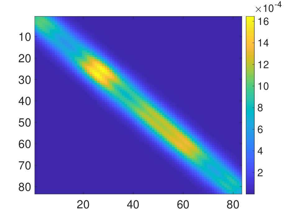
Next we show how to use SQR to make statistical inference. First, we selected one male patient with age $60$ and ADAS $51$ and calculated FA curves at different quantiles along the midsagittal corpus callosum skeleton with the fitted model. Figure 5.9 (a) shows the marginal distribution $Y(s_{j})$ given ${\bf x}=(1,\text{male},\text{age}=60,\text{ADAS}=51)$ . In addition, we plot a subset of subjects having much smaller ADAS scores ( $<10$ ) in red in Figure 5.9 (a). From this plot, we see that, in general, people with smaller ADAS scores have higher FA values than the one with ADAS $=51$ . FA represents white matter integrity. A smaller FA along the midsagittal corpus callosum indicates deteriorations of the corpus callosum fiber bundle, and thus weakened bilateral communications. Our finding is consistent with the literature (Biegon et al. 1994; Ardekani et al. 2014). Second, we carried out statistical inference using $p$ -values. Figure 5.9 (b) shows the p-value curve of the subject with ADAS=8 under the estimated marginal distribution of the subject with ADAS=51. In most locations, the FA value differs significantly from the two subjects ( $1-p<0.05$ ). Third, Figure 5.10 shows more results obtained from the copula model, where panels (a) and (b) show $\varrho/(\varrho-2)\widehat{\boldsymbol{\Sigma}}_{\boldsymbol{\theta}({\bf x}_{1})}$ and $\varrho/(\varrho-2)\widehat{\boldsymbol{\Sigma}}_{\boldsymbol{\theta}({\bf x}_{2})}$ for ${\bf x}_{1}=$ (male, age $=61$ , ADAS $=5$ ) and ${\bf x}_{2}=$ (male, age $=60$ , ADAS $=51$ ), respectively, panel (c) shows their difference, and panel (d) shows random samples simulated from the distributions of $Y|{\bf x}_{1}$ (blue) and $Y|{\bf x}_{2}$ (red). The covariance matrices $\varrho/(\varrho-2)\widehat{\boldsymbol{\Sigma}}_{\boldsymbol{\theta}({\bf x})}$ and their difference in panels (a) (b) and (c) reveal that subjects with large ADAS values have longer range correlation between $t_{\varrho}^{-1}(u_{i})$ and $t^{-1}_{\varrho}(u_{j})$ at certain locations, indicating that they have more smoothed FA curves compared with those with small ADAS values. Moreover, the results in panel (d) reveals that healthy subjects in general have higher FA values than AD subjects with the same age and gender.

5.3.2 Hippocampus Surface Data

In another example, we analyze the hippocampal substructures extracted from MRI scans in the ADNI study. The hippocampus locates in the medial temporal lobe underneath the cortical surface. It belongs to the limbic system and plays important roles in the consolidation of information from short-term memory to long-term memory and spatial navigation (Colom et al. 2013; Luders et al. 2013). The neurodegenerative activity of AD is evident in the hippocampus region.

In our study, given the MRI scans, the hippocampal substructures were segmented with FSL FIRST (Patenaude et al. 2011) and the hippocampal surfaces were automatically reconstructed with the marching cube method (Lorensen and Cline 1987). We used a surface fluid registration based hippocampal subregional analysis package (Wang et al. 2011; Shi et al. 2013; Shi et al. 2014) that uses isothermal coordinates and fluid registration to generate the correspondence between hippocampal surfaces and the statistics computed on the surface. This method introduces two cuts on a hippocampal surface to convert it into a genus zero surface with two open boundaries. The locations of the two cuts were at the front and back of the hippocampal surface. By using conformal parameterization, it converts a 3D surface registration problem into a 2D image registration problem. The flow induced in the parameter domain establishes high-order correspondences between 3D surfaces. After the registration, various surface statistics were computed on the registered surface, such as multivariate tensor-based morphometry statistics (Wang et al. 2011) that retain the full tensor information of the deformation Jacobian matrix, and the radial distance (Pizer et al. 1999). This software package has been applied in various studies (Wang et al. 2011; Wang et al. 2013; Shi et al. 2013; Shi et al. 2014). The radial distance feature is used in this paper. An example of one subject’s left and right hippocampus images are shown in Figure 5.11, where the left side of (a) or (b) corresponds to the bottom of the hippocampus in (c), and the right side corresponds to the top.

We applied our SQR to the hippocampus data set. We have $403$ subjects, $223$ of which are healthy controls (107 females and 116 males), and 180 of which have AD ( 87 females and 93 males). Scalar covariates include the subject’s gender, age, and behavior score ( $1$ - $36$ , where lower scores correspond to healthy controls and higher scores corresponds to ADs). The response variable is the 2D hippocampus image. Preliminary analysis indicates that gender does not have a significant effect on hippocampus and therefore, in our analysis, we only include two covariates – age and behavior score, both of which are normalized. In the following, we present results for the right hippocampal surfaces. Figure 5.12 shows the coefficient images at $\tau=0.5$ , with more results for $\tau=0.25$ and $0.75$ shown in Figure 2.1 in the Supplement II. Our results indicate that both aging and AD will degenerate the hippocampus, especially the bottom part, and the AD has more adverse effect than the aging (Scher et al. 2007; Frisoni et al. 2008).

In another experiment, we compared marginal distributions given different covariates. We first got the marginal distribution $Y(s)|{\bf x}=(1.47,2.48)$ (corresponding to age = 85, behavior = 30.3) and then calculated the p-value maps of some randomly selected observations $Y_{i}$ . The results are shown in Figure 5.13. We can see that the hippocampus in younger adults with good behavior scores have significantly bigger hippocampus (especially the part close to the bottom) than subjects with age 85 and behavior 30.3.

6 Discussions

We have developed a class of SQR models for function-on-scalar regression, which explicitly characterizes the conditional spatial distribution of a high-dimensional functional/image response given scalar predictors. We have borrowed the strength from both quantile regression and copula modeling, and have developed an efficient primal-dual algorithm to estimate unknown parameters. Simulations and real data analysis are used to show that SQR is efficient to obtain a comprehensive understanding of the effect of scalar covariates on the functional response at different quantile levels. We also established the optimal rate of convergence on the estimation of the coefficient functions.

Many important issues need to be addressed in future research. First, although we focus on the analysis of one- and two-dimensional images, it is straightforward to apply our methods to $k$ -dimensional images with $k>2$ . Under this circumstance, the coefficient functions $\beta_{\tau}(\cdot)$ are $k$ -dimensional unknown functions, and the spatial location sampling frequency $m$ will be much larger than that of two-dimensional images. In this case, the computational efficiency is the key challenge. Second, instead of analyzing image data in a raw space directly, we may achieve better results by working on a transformed space, such as frequency. In this case, some further development may be necessary. Third, it is interesting to consider several alternatives to the quantile used in this paper. For instance, we may consider a new multivariate concept of quantile based on a directional version of Koenker and Bassett’s traditional regression quantiles for multivariate location and multiple-output regression problems (Koenker et al. 2017). In their empirical version, those quantiles can be computed efficiently via linear programming techniques. The contours generated by those quantiles are shown to coincide with the classical halfspace depth contours associated with the name of Tukey. This depth approach is an interesting alternative and we will leave it for future research.

References

Ardekani et al. (2014) Ardekani, B. A., A. H. Bachman, K. Figarsky, and J. J. Sidtis (2014). Corpus callosum shape changes in early Alzheimer’s disease: an MRI study using the OASIS brain database. Brain Structure and Function 219(1), 343–352.
Bárdossy (2006) Bárdossy, A. (2006). Copula-based geostatistical models for groundwater quality parameters. Water Resources Research 42(11).
Biegon et al. (1994) Biegon, A., J. Eberling, B. Richardson, M. Roos, S. Wong, B. R. Reed, and W. Jagust (1994). Human corpus callosum in aging and Alzheimer’s disease: a magnetic resonance imaging study. Neurobiology of aging 15(4), 393–397.
Bouyé and Salmon (2013) Bouyé, E. and M. Salmon (2013). Dynamic copula quantile regressions and tail area dynamic dependence in forex markets. Copulae and Multivariate Probability Distributions in Finance, 125–154.
Bowman (2010) Bowman, A. (2010). Functional data analysis with R and MATLAB. Journal of Statistical Software 34(1), 1–2.
Boyd et al. (2011) Boyd, S., N. Parikh, E. Chu, B. Peleato, and J. Eckstein (2011). Distributed optimization and statistical learning via the alternating direction method of multipliers. Foundations and Trends® in Machine learning 3(1), 1–122.
Cai and Hall (2006) Cai, T. and P. Hall (2006). Prediction in functional linear regression. The Annals of Statistics, 34(5), 2159–2179.
Cai and Yuan (2012) Cai, T. T. and M. Yuan (2012). Minimax and adaptive prediction for functional linear regression. Journal of the American Statistical Association 107(499), 1201–1216.
Cai and Xu (2008) Cai, Z. and X. Xu (2008). Nonparametric quantile estimations for dynamic smooth coefficient models. Journal of the American Statistical Association 103(484), 1595–1608.
Chen et al. (2009) Chen, X., R. Koenker, and Z. Xiao (2009). Copula based nonlinear quantile autoregression. The Econometrics Journal 12, S50–S67.
Colom et al. (2013) Colom, R., J. L. Stein, P. Rajagopalan, K. Martínez, D. Hermel, Y. Wang, J. Álvarez-Linera, M. Burgaleta, M. Á. Quiroga, P. C. Shih, and P. M. Thompson (2013). Hippocampal structure and human cognition: Key role of spatial processing and evidence supporting the efficiency hypothesis in females. Intelligence 41(2), 129–140.
Crambes et al. (2009) Crambes, C., A. Kneip, and P. Sarda (2009). Smoothing splines estimators for functional linear regression. The Annals of Statistics 37(1), 35–72.
Cressie (1985) Cressie, N. (1985). Fitting variogram models by weighted least squares. Mathematical Geology 17(5), 563–586.
Cressie (2015) Cressie, N. A. (2015). Statistics for Spatial Data, Revised Edition. Wiley.
De Angelis et al. (1997) De Angelis, P. L., P. M. Pardalos, and G. Toraldo (1997). Quadratic programming with box constraints. In Developments in Global Optimization, pp. 73–93. Springer.
De Backer et al. (2017) De Backer, M., A. E. Ghouch, and I. Van Keilegom (2017). Semiparametric copula quantile regression for complete or censored data. Electronic Journal of Statistics 11, 1660–1698.
Demarta and McNeil (2005) Demarta, S. and A. J. McNeil (2005). The t copula and related copulas. International statistical review 73(1), 111–129.
Du and Wang (2014) Du, P. and X. Wang (2014). Penalized likelihood functional regression. Statistica Sinica 24(2), 1017–1041.
Efron (1986) Efron, B. (1986). How biased is the apparent error rate of a prediction rule? Journal of the American Statistical Association 81(394), 461–470.
Ferraty and Vieu (2006) Ferraty, F. and P. Vieu (2006). Nonparametric Functional Data Analysis: Methods, Theory, Applications and Implementations. Springer.
Frisoni et al. (2008) Frisoni, G. B., R. Ganzola, E. Canu, U. Rüb, F. B. Pizzini, F. Alessandrini, G. Zoccatelli, A. Beltramello, C. Caltagirone, and P. M. Thompson (2008). Mapping local hippocampal changes in Alzheimer’s disease and normal ageing with MRI at 3 Tesla. Brain 131(12), 3266–3276.
Genton (1998) Genton, M. G. (1998). Variogram fitting by generalized least squares using an explicit formula for the covariance structure. Mathematical Geology 30(4), 323–345.
Goldsmith and Kitago (2016) Goldsmith, J. and T. Kitago (2016). Assessing systematic effects of stroke on motor control by using hierarchical function-on-scalar regression. Journal of the Royal Statistical Society: Series C (Applied Statistics) 65(2), 215–236.
Greven and Scheipl (2017) Greven, S. and F. Scheipl (2017). A general framework for functional regression modelling. Statistical Modelling 17(1-2), 1–35.
Gutenbrunner and Jurecková (1992) Gutenbrunner, C. and J. Jurecková (1992). Regression rank scores and regression quantiles. The Annals of Statistics, 305–330.
Gutenbrunner et al. (1993) Gutenbrunner, C., J. Jurečková, R. Koenker, and S. Portnoy (1993). Tests of linear hypotheses based on regression rank scores. Journaltitle of Nonparametric Statistics 2(4), 307–331.
Guttorp and Gneiting (2006) Guttorp, P. and T. Gneiting (2006). Studies in the history of probability and statistics XLIX on the Matérn correlation family. Biometrika 93(4), 989–995.
Hall and Horowitz (2007) Hall, P. and J. L. Horowitz (2007). Methodology and convergence rates for functional linear regression. The Annals of Statistics 35(1), 70–91.
Hallin et al. (2009) Hallin, M., Z. L. Lu, and K. Yu (2009). Local linear spatial quantile regression. Bernoulli, 659–686.
Inano et al. (2011) Inano, S., H. Takao, N. Hayashi, O. Abe, and K. Ohtomo (2011). Effects of age and gender on white matter integrity. American Journal of Neuroradiology 32(11), 2103–2109.
Ivanescu et al. (2015) Ivanescu, A. E., A.-M. Staicu, F. Scheipl, and S. Greven (2015). Penalized function-on-function regression. Computational Statistics 30(2), 539–568.
Kato et al. (2012) Kato, K. et al. (2012). Estimation in functional linear quantile regression. The Annals of Statistics 40(6), 3108–3136.
Kazianka and Pilz (2010) Kazianka, H. and J. Pilz (2010). Copula-based geostatistical modeling of continuous and discrete data including covariates. Stochastic Environmental Research and Risk Assessment 24(5), 661–673.
Koay et al. (2006) Koay, C. G., L.-C. Chang, J. D. Carew, C. Pierpaoli, and P. J. Basser (2006). A unifying theoretical and algorithmic framework for least squares methods of estimation in diffusion tensor imaging. Journal of Magnetic Resonance 182(1), 115–125.
Kochunov et al. (2007) Kochunov, P., P. M. Thompson, J. L. Lancaster, G. Bartzokis, S. Smith, T. Coyle, D. R. Royall, A. Laird, and P. T. Fox (2007). Relationship between white matter fractional anisotropy and other indices of cerebral health in normal aging: tract-based spatial statistics study of aging. Neuroimage 35(2), 478–487.
Koenker (2004) Koenker, R. (2004). Quantile regression for longitudinal data. Journal of Multivariate Analysis 91(1), 74–89.
Koenker (2005) Koenker, R. (2005). Quantile Regression. Cambridge University Press.
Koenker and Bassett Jr (1978) Koenker, R. and G. Bassett Jr (1978). Regression quantiles. Econometrica 46(1), 33–50.
Koenker et al. (2017) Koenker, R., V. Chernozhukov, X. He, and L. Peng (2017). Handbook of Quantile Regression. Chapman and Hall/CRC.
Koenker et al. (1994) Koenker, R., P. Ng, and S. Portnoy (1994). Quantile smoothing splines. Biometrika 81(4), 673–680.
Koenker and Park (1996) Koenker, R. and B. J. Park (1996). An interior point algorithm for nonlinear quantile regression. Journal of Econometrics 71, 265–283.
Kostov (2009) Kostov, P. (2009). A spatial quantile regression hedonic model of agricultural land prices. Spatial Economic Analysis 4(1), 53–72.
Kraus and Czado (2017) Kraus, D. and C. Czado (2017). D-vine copula based quantile regression. Computational Statistics & Data Analysis 110, 1–18.
Lahiri et al. (2002) Lahiri, S. N., Y. Lee, and N. Cressie (2002). On asymptotic distribution and asymptotic efficiency of least squares estimators of spatial variogram parameters. Journal of Statistical Planning and Inference 103(1-2), 65–85.
Li et al. (2007) Li, Y., Y. Liu, and J. Zhu (2007). Quantile regression in reproducing kernel hilbert spaces. Journal of the American Statistical Association 102(477), 255–268.
Lorensen and Cline (1987) Lorensen, W. E. and H. E. Cline (1987). Marching cubes: A high resolution 3D surface construction algorithm. In ACM Siggraph Computer Graphics, Volume 21, pp. 163–169.
Lu et al. (2014) Lu, Z., Q. Tang, and L. Cheng (2014, 02). Estimating spatial quantile regression with functional coefficients: A robust semiparametric framework. Bernoulli 20(1), 164–189.
Luders et al. (2013) Luders, E., P. M. Thompson, F. Kurth, J.-Y. Hong, O. R. Phillips, Y. Wang, B. A. Gutman, Y.-Y. Chou, K. L. Narr, and A. W. Toga (2013). Global and regional alterations of hippocampal anatomy in long-term meditation practitioners. Human Brain Mapping 34(12), 3369–3375.
Matérn (2013) Matérn, B. (2013). Spatial Variation, Volume 36. Springer-Verlag New York.
Matheron (1963) Matheron, G. (1963). Principles of geostatistics. Economic Geology 58(8), 1246–1266.
Meyer and Woodroofe (2000) Meyer, M. and M. Woodroofe (2000). On the degrees of freedom in shape-restricted regression. Annals of Statistics, 1083–1104.
Nikoloulopoulos et al. (2012) Nikoloulopoulos, A. K., H. Joe, and H. Li (2012). Vine copulas with asymmetric tail dependence and applications to financial return data. Computational Statistics & Data Analysis 56(11), 3659–3673.
Patenaude et al. (2011) Patenaude, B., S. M. Smith, D. N. Kennedy, and M. Jenkinson (2011). A Bayesian model of shape and appearance for subcortical brain segmentation. Neuroimage 56(3), 907–922.
Pizer et al. (1999) Pizer, S. M., D. S. Fritsch, P. A. Yushkevich, V. E. Johnson, and E. L. Chaney (1999). Segmentation, registration, and measurement of shape variation via image object shape. IEEE Transactions on Medical Imaging 18(10), 851–865.
Portnoy (1997) Portnoy, S. (1997). On computation of regression quantiles: Making the Laplacian tortoise faster. Lecture Notes-Monograph Series, 187–200.
Portnoy and Koenker (1997) Portnoy, S. and R. Koenker (1997). The Gaussian hare and the Laplacian tortoise: computability of squared-error versus absolute-error estimators. Statistical Science 12, 279–300.
Ramsay and Silverman (2005) Ramsay, J. O. and B. W. Silverman (2005). Functional Data Analysis. Springer-Verlag New York.
Ramsay and Silverman (2007) Ramsay, J. O. and B. W. Silverman (2007). Applied Functional Data Analysis: Methods and Case Studies. Springer-Verlag New York.
Reich (2012) Reich, B. J. (2012). Spatiotemporal quantile regression for detecting distributional changes in environmental processes. Journal of the Royal Statistical Society: Series C (Applied Statistics) 61(4), 535–553.
Reich et al. (2011) Reich, B. J., M. Fuentes, and D. B. Dunson (2011). Bayesian spatial quantile regression. Journal of the American Statistical Association, 6–20.
Reiss et al. (2010) Reiss, P. T., L. Huang, and M. Mennes (2010). Fast function-on-scalar regression with penalized basis expansions. The International Journal of Biostatistics 6(1).
Rosen et al. (1984) Rosen, W. G., R. C. Mohs, and K. L. Davis (1984). A new rating scale for Alzheimer’s disease. The American Journal of Psychiatry 141(11), 1356–1364.
Scher et al. (2007) Scher, A., Y. Xu, E. Korf, L. White, P. Scheltens, A. Toga, P. Thompson, S. Hartley, M. Witter, D. Valentino, and L. Launer (2007). Hippocampal shape analysis in Alzheimer’s disease: a population-based study. Neuroimage 36(1), 8–18.
Schwarz (1978) Schwarz, G. (1978). Estimating the dimension of a model. The Annals of Statistics 6(2), 461–464.
Shi et al. (2014) Shi, J., N. Lepore, B. A. Gutman, P. M. Thompson, L. C. Baxter, R. J. Caselli, and Y. Wang (2014). Genetic influence of apolipoprotein E4 genotype on hippocampal morphometry: An N=725 surface-based Alzheimer’s disease neuroimaging initiative study. Human Brain Mapping 35(8), 3903–3918.
Shi et al. (2013) Shi, J., P. M. Thompson, B. Gutman, and Y. Wang (2013). Surface fluid registration of conformal representation: Application to detect disease burden and genetic influence on hippocampus. NeuroImage 78, 111–134.
Smith et al. (2006) Smith, S. M., M. Jenkinson, H. Johansen-Berg, D. Rueckert, T. E. Nichols, C. E. Mackay, K. E. Watkins, O. Ciccarelli, M. Z. Cader, P. M. Matthews, and T. E. Behrens (2006). Tract-based spatial statistics: Voxelwise analysis of multi-subject diffusion data. NeuroImage 31(4), 1487 – 1505.
Stein (1981) Stein, C. M. (1981). Estimation of the mean of a multivariate normal distribution. The Annals of Statistics 9(6), 1135–1151.
Su and Yang (2007) Su, L. and Z. Yang (2007). Instrumental variable quantile estimation of spatial autoregressive models. Development Economics Working Papers 22476, East Asian Bureau of Economic Research.
Sun et al. (2018) Sun, X., P. Du, X. Wang, and P. Ma (2018). Optimal penalized function-on-function regression under a reproducing kernel Hilbert space framework. Journal of the American Statistical Association (DOI: 10.1080/01621459.2017.1356320).
Wahba (1990) Wahba, G. (1990). Spline Models for Observational Data, Volume 59. SIAM.
Wang et al. (2019) Wang, H. J., X. Feng, and C. Dong (2019). Copula-based quantile regression for longitudinal data. Statistica Sinica 29, 245–264.
Wang et al. (2009) Wang, H. J., Z. Zhu, and J. Zhou (2009). Quantile regression in partially linear varying coefficient models. The Annals of Statistics 37(6B), 3841–3866.
Wang et al. (2017) Wang, X., H. Zhu, and A. D. N. Initiative (2017). Generalized scalar-on-image regression models via total variation. Journal of the American Statistical Association 112(519), 1156–1168.
Wang et al. (2011) Wang, Y., Y. Song, P. Rajagopalan, T. An, K. Liu, Y.-Y. Chou, B. Gutman, A. W. Toga, and P. M. Thompson (2011). Surface-based TBM boosts power to detect disease effects on the brain: an N=804 ADNI study. Neuroimage 56(4), 1993–2010.
Wang et al. (2013) Wang, Y., L. Yuan, J. Shi, A. Greve, J. Ye, A. W. Toga, A. L. Reiss, and P. M. Thompson (2013). Applying tensor-based morphometry to parametric surfaces can improve MRI-based disease diagnosis. Neuroimage 74, 209–230.
Wyss-Coray (2016) Wyss-Coray, T. (2016). Ageing, neurodegeneration and brain rejuvenation. Nature 539(7628), 180–186.
Yang and He (2015) Yang, Y. and X. He (2015). Quantile regression for spatially correlated data: An empirical likelihood approach. Statistica Sinica, 261–274.
Yao et al. (2005) Yao, F., H.-G. Müller, and J.-L. Wang (2005). Functional linear regression analysis for longitudinal data. The Annals of Statistics, 2873–2903.
Yi and He (2009) Yi, G. Y. and W. He (2009). Median regression models for longitudinal data with dropouts. Biometrics 65(2), 618–625.
Yuan (2006) Yuan, M. (2006). GACV for quantile smoothing splines. Computational Statistics & Data Analysis 50(3), 813–829.
Yuan et al. (2010) Yuan, M., T. T. Cai, et al. (2010). A reproducing kernel Hilbert space approach to functional linear regression. The Annals of Statistics 38(6), 3412–3444.
Zhu et al. (2011) Zhu, H., L. Kong, R. Li, M. Styner, G. Gerig, W. Lin, and J. H. Gilmore (2011). FADTTS: functional analysis of diffusion tensor tract statistics. NeuroImage 56(3), 1412–1425.
Zhu et al. (2007) Zhu, H., H. Zhang, J. G. Ibrahim, and B. S. Peterson (2007). Statistical analysis of diffusion tensors in diffusion-weighted magnetic resonance imaging data. Journal of the American Statistical Association 102(480), 1085–1102.


(a) Ground truth	(b) Gold standard	(c) GACV	(d) Quantile functions


(a) $\Phi^{-1}(U(s))$	(b) $\widehat{\Phi}^{-1}(U(s))$	(c) truth cov	(d) estimated cov


(62,3.3)	(70,3)	(66,2.7)

(66,2.7)	(70,5.3)	(53,4)


(a) Simulated $\beta^{\mu}$ ’s	(b) Simulated $\beta^{\sigma}$ ’s	(c) Simulated $Y$ under the copula model


(a) Samples using ground truth parameters	(b) Samples using estimated parameters