Lifetimes of (near) eternal false vacua

In quantum mechanics, we are used to the idea that excited states cannot decay provided they are exact eigenstates of the Hamiltonian. If the Hamiltonian enjoys some global symmetry $G$, then there are no transitions between an excited state carrying global charge to a lower energy zero charge state such as the vacuum. In this sense, the notion of an ‘eternal false vacuum’ is somewhat trivial in quantum mechanics.

For instance, consider a particle in a symmetric double-well potential. The spectrum organizes itself into representations of parity, which acts as $x\to-x$. The ground state is the symmetric combination of node-less wave functions localized at the two wells, and is invariant under parity. The first excited state is the anti-symmetric combination, which is odd under parity. On top of each of these states is a tower of excitations, each being even or odd under parity. We may view each tower as being distinct universes, in the sense that they are protected by a selection rule: only parity odd operators can connect states between the two sectors. (Of course, the excited states within each tower cannot decay either, since they are energy eigenstates.)

Going back to generalities, suppose the system has a second global symmetry $G^{\prime}$ which has a mixed ’t Hooft anomaly with $G$. As a consequence, the ground state can not be unique. We can choose a basis such that the lowest energy states are eigenstates of $G$, but not $G^{\prime}$ (they form a $G^{\prime}$ multiplet). In this way, the symmetry $G^{\prime}$, together with the ’t Hooft anomaly, ensure that the universes associated with $G$ are degenerate. If we break $G^{\prime}$ explicitly this degeneracy is lost, though the universes remain.

An example of the above situation is furnished by a free particle on a circle with a $\theta$-angle Gaiotto:2017yup; Kikuchi:2017pcp; Aitken:2018kky. At $\theta=\pi$ there is a ’t Hooft anomaly between the $U(1)$ shift symmetry and charge conjugation, which together comprise an $O(2)$ symmetry. This symmetry is projectively realized on the Hilbert space. The spectrum consists of states $|n\rangle$ labeled by their $U(1)$ charge. According to the discussion above, each state is its own universe. The two lowest-energy universes $|0\rangle$ and $|1\rangle$ are degenerate and are exchanged by charge conjugation. Once we break charge conjugation by moving away from $\theta=\pi$, one of these states becomes the true vacuum. However, the $U(1)$ symmetry prohibits the decay of the higher-energy states to this unique vacuum.

The discussion so far serves to show that in quantum mechanics, universes and eternal false vacua are overly-complicated ways of thinking about completely standard concepts. However, it will be useful to consider an additional quantum-mechanical example in more detail. The following model exhibits many of the features of the quantum field theories discussed later in the paper.

Consider a quantum mechanical system consisting of three particles with coordinates are $x,y,z$ respectively on a circle of radius $2\pi L$ with Euclidean-time Lagrangian

where we took units where $L=1$ and $p\in{\mathbb{Z}}_{\geq 0}$.²² 2 This model is related to the small-circle limit of the charge-$p$ Schwinger model on $\mathbb{R}\times S^{1}$ which appears in Komargodski:2017dmc. For the precise connection between two-dimensional abelian theories with non-minimal charge and modified instanton sums, see Sec. 3.2. We assume that the $x$ and $z$ periodicities in the potential are $2\pi/p$ and the $y$ periodicity in the potential is $2\pi$. Although the variables $\chi$ and $z$ do not have kinetic terms, they are dynamical in the sense that we integrate over all configurations of $\chi$ and $z$ in the path integral. The $2\pi$-periodic variable $\chi$ plays the role of a Lagrange multiplier setting $\dot{y}=p\,\dot{z}$. Consequently, winding numbers of $y$ are constrained to be multiples of $p$,

To keep things simple, in the following we will set $V(x,y,z)=V(x)$ below unless specified otherwise. This allows us to demonstrate many features exactly (by integrating out $z$ explicitly, for instance) rather than making general statements and then checking them in perturbation theory.

The equation of motion for $z$ sets $\dot{\chi}=0$, and summing over winding configurations with $\int dz\in 2\pi{\mathbb{Z}}$ sets $\chi=2\pi m/p$ for $m\in{\mathbb{Z}}$. The variable $e^{i\chi}$ is therefore ${\mathbb{Z}}_{p}$-valued, and summing over its discrete values enforces the constraint $\int dy\in 2\pi p\,{\mathbb{Z}}$ as a delta function in the path integral.³³ 3 This constraint on the winding numbers of $y$ still holds when $\chi$ and $z$ have kinetic terms, despite the fact that $\chi$ is no longer a discrete-valued field in this case. For simplicity we set these kinetic terms to zero.

For our purposes the relevant symmetries of the model are the two discrete ${\mathbb{Z}}_{p}$ shift symmetries

The symmetry operator of $({\mathbb{Z}}_{p})_{z}$ is $e^{-i\chi}$, in the sense that

To verify this relation one can write

where $\delta S=i\int dt\,\chi(t)\,\delta(t_{0})$. We can cancel this shift in the action by a shift of $z(t)\to z(t)+\frac{2\pi}{p}\Theta(t-t_{0})$, which leads to

reproducing (4). Since $e^{-i\chi}$ itself is charged under $({\mathbb{Z}}_{p})_{x}$, these two shift symmetries have a mixed ‘t Hooft anomaly Gaiotto:2014kfa. The arguments summarized in the introduction suggest that this ought to give rise to $p$ universes.

To see these distinct universes explicitly, it is convenient to integrate out $y$ and $z$ to isolate the dynamics of $x$. Since neither $y$ nor $z$ appear in the Lagrangian explicitly, we can instead integrate over $\dot{y}$ and $\dot{z}$ at the expense of constraining $\frac{1}{2\pi}\int dy$ and $\frac{1}{2\pi}\int dz$ to be integers. This can be achieved with the discrete delta functions

Integrating out $\dot{y}$ and $\dot{z}$, we find

Upon integrating out the auxiliary fields the partition function becomes highly non-local, decomposing into a sum of partition functions $Z_{m}$ labelled by the corresponding value of the Lagrange multiplier $\chi=2\pi m/p$. The $p$ different terms on the right-hand side of (9) are the universes we advertised earlier.

On the other hand, if we restrict our attention to constant values of $x$ and take the Euclidean time direction to be large, then the effect of integrating out $y,z,\chi$ is to produce a local effective potential,

with degenerate minima related by $({\mathbb{Z}}_{p})_{x}$. On the one hand, these $p$ vacua appear to have matched the ‘t Hooft anomaly between $({\mathbb{Z}}_{p})_{x}$ and $({\mathbb{Z}}_{p})_{z}$. At the same time, the naive quantum-mechanical expectation is that the true ground state of the system is described by the $({\mathbb{Z}}_{p})_{x}$-symmetric linear combination of wave functions localized at each minimum. Put differently, one might expect instantons to lift the $p$-fold degeneracy by a non-perturbative amount. However, there are no instanton configurations connecting the minima of the potential (10). To consider dynamical configurations we must pass to the non-local expression (9), where it becomes obvious that ‘nearest-neighbor instantons’ are not sensible field configurations because they would have to connect different terms in the path integral decomposition (i.e., universes).

An immediate corollary is that the $({\mathbb{Z}}_{p})_{x}$ symmetry is spontaneously broken, contrary to the usual lore prohibiting such a conclusion in quantum mechanics. To see this, let us evaluate the expectation value $\langle e^{ix}\rangle$ with a small $({\mathbb{Z}}_{p})_{x}$-breaking perturbation added to the action, and with time having finite extent $T$,

where $\langle e^{ix}\rangle_{m}$ is the expectation value in the $m$’th universe with free energy $\mathcal{F}_{m}(\epsilon)$. When $\epsilon>0$, the free energy $\mathcal{F}_{0}(\epsilon)<\mathcal{F}_{i}(\epsilon)$ for $i>0$. Taking the limit $T\to\infty$, only a single term in (12) survives,

Finally, taking the symmetry-breaking parameter to zero, we find

so that the $({\mathbb{Z}}_{p})_{x}$ symmetry is spontaneously broken. Note that in coming to this conclusion, the exact decomposition of the path integral into universes was crucial–without it, finite-action instantons would proliferate even in the $T\to\infty$ limit, leading to a unique symmetric ground state. Finally, we note that the $p$ degenerate ground states match the ’t Hooft anomaly between the two ${\mathbb{Z}}_{p}$ symmetries.

We can also see how these degenerate ground states appear from a Hamiltonian perspective. In Minkowski space, the Hamiltonian resulting from the Lagrangian (1) is

In the Hamiltonian formalism the $({\mathbb{Z}}_{p})_{x}$ and $({\mathbb{Z}}_{p})_{z}$ shift symmetries are generated by the operators $\hat{U}_{x}=e^{i\frac{2\pi}{p}\hat{p}_{x}}e^{-i\hat{z}}$ and $\hat{U}_{z}=e^{i\frac{2\pi}{p}\hat{p}_{z}}$, respectively. Let $V(\hat{x},\hat{y},\hat{z})=0$ for simplicity. Then the above Hamiltonian is equivalent to a Landau problem on the torus with $p$ units of magnetic flux Komargodski:2017dmc. The system has $p$ degenerate ground states $|m\rangle$ on the torus identified by their eigenvalues $\hat{U}_{z}|m\rangle=e^{2\pi im/p}\,|m\rangle$ under $({\mathbb{Z}}_{p})_{z}$. The wave functions are

The $p$ ground states have energy $E=g/4\pi$ and are permuted by $({\mathbb{Z}}_{p})_{x}$ as $\hat{U}_{x}|m\rangle=|m-1\rangle$. The symmetry operators therefore satisfy the relation $\hat{U}_{x}\hat{U}_{z}=e^{2\pi i/p}\,\hat{U}_{z}\hat{U}_{x}$ corresponding to a central extension of ${\mathbb{Z}}_{p}\times{\mathbb{Z}}_{p}$ to the Weyl-Heisenberg group. This is the manifestation of the mixed anomaly.

It is important to note that the existence of $p$ universes is protected by the $({\mathbb{Z}}_{p})_{z}$ symmetry alone, and does not rely on the existence of the $({\mathbb{Z}}_{p})_{x}$ symmetry nor the ’t Hooft anomaly between them. To see this, we can again add the $({\mathbb{Z}}_{p})_{x}$-breaking term $\epsilon\cos(x)$ to the Lagrangian. As shown in Figure 1(b), such a term lifts the degeneracy between universes, but the universes remain. Despite the fact that we can make the difference in energy densities between neighboring vacua large by increasing $\epsilon$, if we prepare the system in one of the false vacuum states it cannot tunnel into the true vacuum. Hence, the false vacua are eternal.

On the other hand, we can leave $({\mathbb{Z}}_{p})_{x}$ intact and break the $({\mathbb{Z}}_{p})_{z}$ symmetry explicitly by (for example) including a $V(\hat{x},\hat{y},\hat{z})=\cos(\hat{z})$ potential,

This leaves a single universe with degenerate vacua related by the remaining $({\mathbb{Z}}_{p})_{x}$ symmetry. Since these vacua now exist in the same universe, finite-action tunneling events will proliferate and give rise to a unique symmetric vacuum. In fact, the ground state remains unique even as we take $\mu\to 0$. On the other hand, we know that when $\mu$ is strictly vanishing there are $p$ degenerate ground states.

To see this explicitly we can treat the variable $x$ within the Born-Oppenheimer approximation. Integrating out the ‘fast’ mode $z$ gives an effective potential for $x$ which is the analog of Eq. (10) when the $({\mathbb{Z}}_{p})_{z}$ symmetry is broken. The Born-Oppenheimer approximation is justified as long as the curvature of the induced effective potential is smaller than $\sqrt{p}\,\mu$, which can easily be arranged. Though the $({\mathbb{Z}}_{p})_{z}$-breaking potential is non-linear, this process can be done numerically. As shown in Figure 1(c), the level-crossings are avoided and the spectrum organizes itself into bands. Within the lowest band, instantons proliferate and give rise to a unique ground state. We can even compute the instanton action for nearest-neighbor tunneling in the limit $\mu\to 0$. In this limit the effective potential reduces to (10). When $V(x)=0$, the instanton action is $S_{I}=\frac{\pi}{2p^{2}}$, which clearly shows no singularity as $\mu\to 0$. Again, this signals a non-uniformity in the symmetry-restoring limit: we know from our above arguments that $\mu=0$ is a distinguished point in parameter space where tunneling is completely suppressed, i.e. where $S_{I}$ is infinite.

The Euclidean Lagrangian of the massless charge-$p$ Schwinger model is

where $f_{\mu\nu}=\partial_{\mu}a_{\nu}-\partial_{\nu}a_{\mu}$. We assume that the theory is defined on a closed 2-manifold so that the topological charges are quantized as

The theory has a ${\mathbb{Z}}_{2p}^{(0)}$ 0-form chiral symmetry, but the ${\mathbb{Z}}_{2}$ subgroup generated by $(-1)^{F}$ is actually non-chiral and lies within the $U(1)$ gauge group. We will focus on the faithfully acting ${\mathbb{Z}}_{p}^{(0)}={\mathbb{Z}}_{2p}^{(0)}/\mathbb{Z}_{2}$ chiral symmetry below. The theory also has a 1-form ${\mathbb{Z}}_{p}^{(1)}$ center symmetry. The bosonized form of the massless charge-$p$ Schwinger model is PhysRevD.11.2088; Coleman:1976uz

where we have switched to form notation, so that $a=a_{\mu}dx^{\mu}$ and used the shorthand $|\omega|^{2}=\omega\wedge\star\omega$. Here $\varphi$ is a $2\pi$-periodic scalar and the discrete chiral symmetry becomes the shift symmetry $\varphi\to\varphi+2\pi/p$. The 1-form ${\mathbb{Z}}_{p}^{(1)}$ symmetry acts by shifting $a\to a+\lambda$ by a flat connection with $\int\lambda=2\pi{\mathbb{Z}}/p$. The ${\mathbb{Z}}_{p}^{(0)}$ and ${\mathbb{Z}}_{p}^{(1)}$ symmetries have a mixed anomaly Anber:2018jdf; Misumi:2019dwq; Armoni:2018bga, which can be seen by turning on an appropriate background 2-form gauge field for the 1-form symmetry.

An important point is that the symmetry operator of the $1$-form symmetry is a local operator, which up to a normalization constant is given by $U_{m}(x)=e^{i\frac{2\pi m}{p}\left(-\frac{i}{e^{2}}\star da+\frac{p}{2\pi}\varphi\right)}$. Indeed, the equation of motion for the gauge field can be written as

The 0-form expression in parentheses is therefore a conserved quantity, and this can be used to show that $U_{m}(x)$ is a well-defined local topological operator so long as $m\in\mathbb{Z}$. The symmetry operator satisfies

where the linking number $\ell(C,x)=0$ or $1$ depending on if the point $x$ is inside the closed contour $C$, which we take to be oriented and without self-intersections. So long as the 1-form symmetry is not explicitly broken, correlation functions of $U_{m}(x)$ should be topological — which in the case of local operators, means independent of the position $x$. We will see that this enforces strict constraints on the possible dynamical domain wall configurations in which $\varphi$ approaches distinct values at asymptotic infinity. In particular, domain wall configurations where $U_{m}(x)$ depends on spacetime necessarily have infinite tension. While one can consider such domain walls as probes of the theory, they are not dynamical excitations Komargodski:2020mxz.

In the deep IR limit $e^{2}\to\infty$, integrating out $a$ locally sets $d\varphi=0$, while the sum over topologically non-trivial sectors (global fluxes $\int da\in 2\pi{\mathbb{Z}}$) results in the constraint $\varphi=2\pi\ell/p$, with $\ell\in{\mathbb{Z}}$. The field $\varphi$ is frozen to one of $p$ values, and there are no domain walls which interpolate between them. In this limit the distinct values $\ell\in\{0,\ldots,p-1\}$ label distinct universes. Even away from the extreme IR limit the theory (20) is Gaussian and we can integrate out the gauge field by treating $F=da$ as the fundamental degree of freedom. Imposing $U(1)$ flux quantization (read: the Bianchi identity) as a delta function constraint,

the path integral can be expressed as

There is no longer a local effective Lagrangian for $\varphi$: the partition function decomposes into a sum of distinct path integrals labelled by the integer $k$.⁴⁴ 4 If we decompose $k=p\,n+\ell$, where $n\in{\mathbb{Z}}$ and $\ell\in\{0,\ldots,p-1\}$, then $\ell$ can be interpreted as a discrete theta parameter of the charge-$p$ Schwinger model with the ${\mathbb{Z}}_{p}^{(1)}$ 1-form symmetry gauged. At a technical level, minimizing over $n$ ensures that the potential is $2\pi$-periodic with respect to $\varphi$ while the minimization over $\ell$ ensures the potential is $2\pi$-periodic with respect to $\theta$. The $p$ inequivalent terms in the above decomposition are distinct universes, labelled by the expectation value of the $1$-form symmetry operator $\langle U_{1}(x)\rangle=e^{2\pi ik/p}$.

In the infinite volume limit, the potential for the zero mode of $\varphi$, which we denote $\varphi_{0}$, can be written in a manifestly local way as

The potential in Eq. (25) has $p$ degenerate minima corresponding to $\varphi_{0}=(2\pi k-\theta)/p$. These minima are related by the ${\mathbb{Z}}_{p}^{(0)}$ discrete shift symmetry, which is spontaneously broken. We emphasize that each chiral vacuum lies in a distinct universe. Hence, dynamical domain walls between neighboring vacua do not exist as they violate the ‘topological’ property of the operator $U_{m}(x)$ (which is protected by the absence of charge-$1$ matter and the resulting 1-form ${\mathbb{Z}}_{p}^{(1)}$ symmetry). As a result, these states do not mix even when spacetime is compact: they belong to different universes. At the technical level, domain walls cannot exist because each ${\mathbb{Z}}_{p}^{(0)}$-breaking vacuum lies within a distinct branch of the effective potential.

At the risk of being pedantic, let us explain how spontaneous symmetry breaking occurs in the presence of universes. To conclude that a (0-form) symmetry is spontaneously broken one works in a large but finite spatial volume $V$ and introduces a symmetry-breaking perturbation at some scale $m$ which is small compared to the intrinsic scales (inverse correlation length) of the problem. Normally, we say that a symmetry is spontaneously broken when

for some local operator $\mathcal{O}$ which transforms under the symmetry. Importantly, the limits above do not commute, and it is always true that $\lim_{V\to\infty}\lim_{m\to 0}\langle\mathcal{O}\rangle=0$.

In the context of the Schwinger model, $m$ is a small chiral symmetry-breaking mass for the fermion, with the $\theta$ parameter absorbed into the phase of the fermion mass by a chiral rotation, $\arg(m)=\theta/p$. Using Eq. (24) we can write the expectation value of $e^{i\varphi}\sim\bar{\psi}_{L}\psi_{R}$ as

where $\langle e^{i\varphi}\rangle_{k}$ is the expectation value in the universe with action $S_{k}(m)$ and $L$ is the spatial volume. It is useful to trade $Z_{k}$ for the free energy $\mathcal{F}_{k}$ via $Z_{k}(m)=e^{-LT\mathcal{F}_{k}(m)}$, where $LT$ is the spacetime volume. For any given fixed $|m|$ and a generic value $\arg(m)$ the set $\{\mathcal{F}_{k}(m)\}$ has a unique minimum $\mathcal{F}_{\rm k_{\rm min}}(m)$, but of course $k_{\rm min}$ depends on $\arg m$.⁵⁵ 5 When $\theta=\pi$ the minimum of $\{\mathcal{F}_{k}(m)\}$ becomes doubly-degenerate, corresponding to the spontaneous breaking of charge conjugation. We will not consider this special case here. As a result, in the infinite volume limit only a single term in the sum contributes to the expectation value,

where the value of the integer $n$ depends on $\arg m=\theta/p$. If instead we had taken $m\to 0$ before $L\to\infty$, each universe would contribute equally to the expectation value, and we would erroneously conclude that $\langle e^{i\varphi}\rangle=\sum_{k=0}^{p-1}e^{2\pi ik/p}=0$.

We have seen that the ${\mathbb{Z}}_{p}^{(0)}$ chiral symmetry is spontaneously broken in the massless Schwinger model. When the fermion is massless the ${\mathbb{Z}}_{p}^{(1)}$ symmetry is also spontaneously broken. This is easily seen by noticing that the insertion of a charge-$q$ Wilson loop in the path integral shifts the theta angle by $\theta\to\theta-2\pi q$ inside the loop. Hence, inside the loop, the partition function is that of the universe with an unshifted $\theta$ but with $k\to k+q$ relative to the outside. Since the universes are degenerate, the difference in energy density inside and outside the Wilson loop vanishes. As a result there is no area-law contribution to the Wilson loop expectation value, and ${\mathbb{Z}}_{p}^{(1)}$ is spontaneously broken. When the fermion mass $m\not=0$ the theory becomes confining, with string tensions scaling like $m\,e$ or $m^{2}$ depending on whether $|m|\ll e$ or $|m|\gg e$ Komargodski:2020mxz. Of course, when we add charge-$1$ matter to the theory the 1-form symmetry is explicitly broken. In the following, we examine both symmetry-breaking perturbations of the massless Schwinger model in more detail.

Let us explicitly introduce a mass for the fermion, so that the bosonized potential is

where $\mu$ is some scale determined by matching to the original fermionic theory. The mass term breaks the ${\mathbb{Z}}_{p}^{(0)}$ symmetry completely, and for generic values of $m,\theta$ there is a unique vacuum. The exception is at $\theta=\pi$, where two ground states emerge as one increases the mass. As an example, consider the $p=1$ case at $\theta=\pi$,

For $m\mu\ll e^{2}$ the potential has a single minimum in the fundamental domain $\varphi_{0}\in(0,2\pi)$ at $\varphi_{0}=\pi$. This minimum lies on the branch labelled by $k=1$. As we increase $m$ past a critical value, the potential develops two ground states related by charge conjugation. As we increase $m$ further, there is another critical value where local minima appear in the $k=0$ and $k=2$ branches, see Figure 3. These metastable vacua can decay to one of the true vacua via a tunneling process. All of the branches can be connected via similar tunneling processes–this is possible because they lie within the same universe.

Let us contrast this to what happens when $p>1$. In Figure 4 we compare the $p=3$ effective potential at $\theta=0$ for zero and nonzero mass. When $m=0$ there are three degenerate ground states which spontaneously break ${\mathbb{Z}}_{3}^{(0)}$. Each degenerate vacuum lies in a distinct universe. As soon as the fermion mass is nonzero the degeneracy is lifted and there is a unique vacuum which lies in the branch labelled by $k=0$ mod $3$. False vacua in different branches cannot decay to the true vacuum and are infinitely long-lived.

The infinite lifetimes of false vacua in the above examples with $p>1$ were protected by the 1-form ${\mathbb{Z}}_{p}^{(1)}$ symmetry. This symmetry is explicitly broken when we introduce matter with minimal charge. To this end, let us introduce a heavy charge-$1$ fermion $\zeta$ with mass $M$, with $M^{2}\gg e^{2}$. When $p$ is even, the $\zeta$ fermion number $(-1)^{F_{\zeta}}$ coincides with a gauge transformation, while when $p$ is odd, the overall fermion number $(-1)^{F}$ lies within the gauge group. Applying abelian bosonization to $\psi\leftrightarrow\varphi$ and $\zeta\leftrightarrow\eta$ Coleman:1976uz, we obtain a description of the theory with the overall fermion number gauged,

where $c$ is an $\mathcal{O}(1)$ constant. Again, we can integrate out the gauge field to obtain the effective potential for the zero-modes of $\varphi$ and $\eta$. This is shown in Figure 5 for $p=3$. The bosonized charge-$1$ fermion provides an extra direction in field space, and the result is that the branches in Figure 4(a) become smoothly connected: they are all part of the same universe.

Unlike when the ${\mathbb{Z}}_{p}^{(0)}$ symmetry is exact, now there are finite tension domain wall configurations connecting discrete chiral vacua. On the domain wall $\eta$ interpolates between $0$ and $2\pi$ while $\varphi$ interpolates between $2\pi/p$ and $0$. As an example, the trajectory for $p=3$ connecting the $(\varphi,\eta)=(2\pi,0)\to(4\pi/3,2\pi)\sim(4\pi/3,0)$ vacua is shown in Figure 6. The domain wall connecting neighboring chiral vacua follows a straight trajectory in field space parameterized by $\varphi(\tau)=\frac{2\pi k}{p}-\alpha(\tau),\eta=p\,\alpha(\tau)$. In terms of $\alpha$, the domain wall is simply a Sine-Gordon kink

with tension $T\sim M$ up to $\mathcal{O}(1)$ factors.

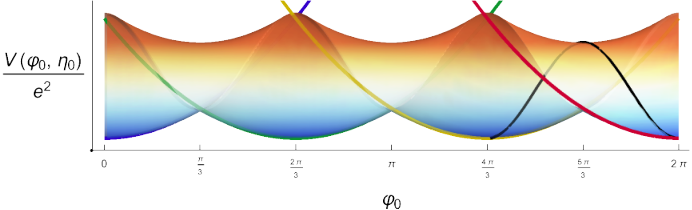
As we increase $M$ the height of the barrier between vacua increases in the smooth direction in field space, while the height of the barrier in the cuspy direction where only $\varphi$ varies stays fixed. When $M$ is large, even though the domain wall passing through the large barrier seems more costly than the domain wall passing through the cusp, the latter configuration is still not admissible. When $M\to\infty$ there are no finite-tension domain walls. Indeed, in the formal limit $M\to\infty$ the unit charge particle decouples and we land on the charge-$p$ model which has $p$ universes.

If we also introduce a mass $m$ for the charge-$p$ fermion the chiral symmetry is broken completely. When $\theta=0$ there is a single unique vacuum at $\varphi=\eta=0$. Unlike the theory without charge-$1$ fields (see Figure 4(b)), the metastable vacua can decay via the nucleation of bubbles of true vacuum.

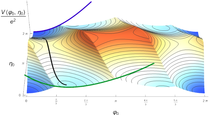
Despite the fact that the false vacuum has an energy density scaling with $m$ relative to the true vacuum, the decay rate can be made arbitrarily small by increasing $M$. The decay rate of the false vacuum scales as $\sim e^{-S_{I}}$ where $S_{I}$ is the action of a bounce solution, which has the form

where $\varepsilon\sim m\mu$ is the difference in energy density of the two minima and $T$ is the tension of the bounce solution, which to leading order in a large $M$ expansion is given by the domain wall tension $T\sim M$. The size of the bubble of true vacuum is $R=T/\epsilon$, so the action of the bounce configuration $S_{I}=\pi T^{2}/\epsilon$ scales as $M^{2}/(m\mu)$ for $M$ large. When $m$ is small compared to $|e|$, $\mu\sim e$. Hence, the lifetime of the false vacuum is exponentially enhanced by the ratio of a ‘UV’ scale $M$ and the low-energy scales $e$ and $m$,

leading to near-eternal false vacua when $M^{2}\gg e\,m$.

So far we have discussed the massless and massive charge-$p$ Schwinger models, and their extensions to include charge-$1$ fermions. Here we provide a different construction that leads to the same physics. As pointed out in Refs. Pantev:2005rh; Seiberg:2010qd, restricting the instanton number in the 2d $\mathbb{C}\mathbb{P}^{N-1}$ model to be a multiple of $p$ gives rise to the same physics as the charge-$p$ $\mathbb{C}\mathbb{P}^{N-1}$ model. Indeed, this correspondence applies to all $U(1)$ gauge theories in two dimensions. For $d>2$ the relation between modified instanton sums and non-minimal charge assignments breaks down. However, theories with modified instanton sums share the features of 2d abelian theories with charge-$p$ matter, namely the existence of universes and false vacua. To set the stage for our treatment of 4d theories with modified instanton sums, we explain the 2d correspondence in detail.

Consider a generic 2d $U(1)$ gauge theory with a charge-$1$ fermion (a nearly identical discussion holds for bosonic matter),

where the ellipses denote other terms allowed by gauge invariance (we do not impose chiral symmetry for the moment). We now modify the theory so that only topological charges which are multiples of $p$ contribute to the partition function Seiberg:2010qd. To this end, let us introduce another $U(1)$ gauge field $\hat{a}$ and a $2\pi$-periodic compact scalar Lagrange multiplier $\chi$, so that the Lagrangian is shifted by

where $\hat{\theta}$ is a new $2\pi$-periodic theta parameter. Integrating out $\chi$ sets $da=p\,d\hat{a}$, which means

so that only topological charges (for $a$) which are multiples of $p$ contribute to the path integral. As a result, $\theta$ has a reduced periodicity, $\theta\sim\theta+2\pi/p$.

On the other hand, the equation of motion for $\hat{a}$ sets $\chi=$ constant, while integrating out $\hat{a}$ and performing the sum over its topological sectors sets $\chi=2\pi k/p$ for $k=0,\ldots,p-1$. The path integral sums over $\ell$, so that

which makes manifest the $2\pi/p$-periodicity of $\theta$.

To see that the charge-$1$ theory with a modified instanton sum is equivalent to the corresponding charge-$p$ theory with a standard instanton sum, we simply solve the local constraint imposed by $\chi$. Substituting $da=p\,d\hat{a}$ into the Lagrangian,

If we now rescale the gauge coupling $e=p\,\hat{e}$, and define $\tilde{\theta}=p\,\theta+\hat{\theta}$, this is just a charge-$p$ $U(1)$ gauge theory with $\theta$ parameter $\tilde{\theta}$ and no modification to the instanton sum. The gauge coupling rescaling is harmless — the only role of $e$ is to set the overall energy scale for the theory.

All of the discussions above are about universes in 2d gauge Abelian gauge theory coupled to charge-$p$ matter applies verbatim to the corresponding theories with minimally-charged matter and modified instanton sums. Uplifting the former construction to higher dimensions only gives rise to a ${\mathbb{Z}}_{p}$ 1-form symmetry, while the latter gives rise to the ${\mathbb{Z}}_{p}$ $(d-1)$-form symmetry necessary for the existence of universes and eternal false vacua.

To make the connection to the charge-$p$ model more explicit, it is worth discussing the 0-form chiral symmetry of the charge-$1$ Schwinger model with a modified instanton sector, whose bosonized form is

Using the arguments in the previous paragraph, this theory is equivalent to the charge-$p$ Schwinger model. One might ask what, in the modified instanton sum description, is the analog of the discrete chiral symmetry ${\mathbb{Z}}_{p}^{(0)}$ of the charge-$p$ Schwinger model. The fact that $e^{i\chi}$ becomes, after integrating out $\hat{a}$, a discrete field valued in the $p$th roots of unity leads to a mild violation of cluster decomposition also observed in the context of ‘Gerby’ conformal field theories Hellerman:2006zs; Pantev:2005rh. Relatedly, the symmetry transformation properties of $e^{i\chi}$ are subtle and should be treated carefully.

In the bosonized variables, a first guess might be to define a shift symmetry which takes $\varphi\to\varphi+2\pi/p$ and does not act on $\chi$. For reference, let us compute the path integral over $\hat{a}$ and $\chi$,