Interior Quasinormal Modes and Strong Cosmic Censorship

Let’s review the 4 dimensional RNdS black hole (see e.g. Wald 1984). This solution of Einstein’s equations describes an electrically charged black hole in a de-Sitter background. The BH is completely specified by 3 parameters, $(M,Q,\Lambda)$, (mass, charge and cosmological constant). In static coordinates $(t,r,\theta,\phi)$, the line element of the metric can be written as:

$$\differential s^{2}\,=\,-\,f\,\differential t^{2}\,+\,\frac{\differential r^{2}}{f}\,+\,r^{2}\,\differential\Omega_{2}^{2},$$

(1)

where $\differential\Omega^{2}$ is the line element of a unit radius $S^{2}$, and

$$f(r)\,=\,1\,-\,\frac{2M}{r}\,+\,\frac{Q^{2}}{r^{2}}\,-\,\frac{\Lambda}{3}\,r^{2}.\\$$

(2)

This spacetime is pathological unless $f(r)$ has 3 positive roots. $r_{-}\leq r_{+}\leq r_{c}$, corresponding to the Cauchy horizon $\mathcal{CH}$, event horizon $\mathcal{H}_{R}$ and cosmological horizon $\mathcal{H}_{C}$. These will bound the different causal regions of the black hole. (see figure 1).

Region I (the black hole exterior), is bounded by $r_{+}\,\leq\,r\,\leq\,r_{c}$. In here $r\,=\,r_{+}$ corresponds to the white hole horizon ($\mathcal{H}^{-}$) at $t=-\infty$ and the right black hole horizon at $t=+\infty$ ($\mathcal{H}_{R}^{+}$). The radial coordinate $r\,=\,r_{c}$ will correspond to the past ($t=-\infty$) and future ($t=+\infty$) cosmological horizons: ($\mathcal{H}_{C}^{-}$ and $\mathcal{H}_{C}^{+}$).

Similarly, region II is bounded by $r_{-}\,\leq\,r\,\leq\,r_{+}$. At $r=r_{-}$ we find the Left ($t=+\infty$) and Right ($t=-\infty$) Cauchy horizons ($\mathcal{CH}_{L}^{+}$ and $\mathcal{CH}_{R}^{+}$ respectively). On the other hand, we have in the causal past $r=r_{+}$, corresponding to the left ($t=-\infty$) and right ($t=+\infty$) future event horizons ($\mathcal{H}_{L}^{+}$ and $\mathcal{H}_{R}^{+}$).

In the calculations that follow, we will work in units such that $\Lambda\,=\,3$. Furthermore, it is instructive to use the roots of f to characterize the black hole (instead of M and Q). To do so, we rewrite (2):

$$f(r)\,=\,-\,\frac{\left(r\,-\,r_{1}\right)\,\left(r\,-\,r_{2}\right)\,\left(r\,-\,r_{3}\right)\,\left(r\,-\,r_{4}\right)}{r^{2}}\quad.$$

(3)

where $r_{i}$ may specify any of the roots of $f$.

To make the structure in (3) explicit, we take $r^{2}f(r)$ in (2) and explicitly evaluate the polynomial quotient with respect to $(r\,-\,r_{1})$. Then, we divide the result by $(r\,-\,r_{2})$. Equating the remainders of this operations to zero, we obtain:

		$\displaystyle M=\,\frac{1}{2}\,\left(r_{1}\,+\,r_{2}\,\right)\,\left(1\,-\,r_{1}^{2}\,-\,r_{2}^{2}\right)$		(4)
		$\displaystyle Q^{2}=\,r_{1}\,r_{2}\,\left(1\,-\,r_{1}\,r_{2}\,-\,r_{1}^{2}\,-\,r_{2}^{2}\right)$		(5)
		$\displaystyle\!\begin{multlined}\frac{r^{2}f(r)}{\left(r\,-\,r_{1}\right)\,\left(r\,-r_{2}\right)}=\\ r^{2}\,+\left(r_{1}\,+\,r_{2}\right)\,r\,+\,r_{1}^{2}\,+\,r_{2}^{2}\,+\,r_{1}\,r_{2}\,\,-\,1\quad.\end{multlined}$

Finally, equating (II.1) to 0, we find that

$$r_{3/4}=-\frac{1}{2}\left(r_{1}\,+\,r_{2}\pm\,\sqrt{4\,-\,2\,r_{1}\,r_{2}\,-\,3\,\left(r_{1}^{2}\,+\,r_{2}^{2}\right)}\right)\\$$

(8)

Lets now define, $r_{1}\,=\,r_{+}$, $r_{2}\,=\,r_{c}$, $r_{3}\,=\,r_{-}$ and $r_{4}\,=\,r_{\tilde{c}}$. Seeking physical solutions, we must impose that the roots $r_{i}$ are real valued, and obey $0\leq r_{-}\leq r_{+}\leq r_{c}$. As we can see in figure 2, this bounds the allowed RNdS black holes by three limiting cases: $r_{-}\,\rightarrow\,0$ (Schwarzschild de Sitter limit), $r_{-}\,\rightarrow\,r_{+}$ (extremal limit) and $r_{+}\,\rightarrow\,r_{c}$ (Nariai limit).

Although $r_{+},\,r_{-}$ and $r_{c}$ are quite useful to discuss properties of the black hole, they are not the best when scanning the BH parameter space (see 2). Instead, it is more intuitive to consider $Q^{2}/Q^{2}_{\text{max}}$ and $y_{+}=r_{+}/r_{c}$. Here, $Q^{2}_{\text{max}}$ is the maximal electric charge for a given value of $y_{+}$. It corresponds to the charge of an extremal RNdS black hole. To obtain this, we take $r_{1}\,=\,r_{3}$ in equation (8), and solve with respect to $r_{1}/r_{2}$. We get:

$$Q^{2}_{\text{max}}=\frac{y_{+}^{2}\,\left(2y_{+}\,+\,1\right)}{\left(3y_{+}^{2}\,+\,2y_{+}\,+\,1\right)^{2}}$$

(9)

These parameters have the advantage of being defined in the interval $(0,\,1)$, transforming the parameter space into a square. Given equations (4) and (5), we may invert the definitions of $y_{+}$ and $Q^{2}/Q_{\text{max}}^{2}$ to obtain $r_{+/-/c}$ as a function of $y_{+}$ and $Q^{2}/Q_{\text{max}}^{2}$.

In the calculations below, we will also make use of the tortoise coordinate, defined through:

$$\differential r_{*}=\frac{\differential r}{f(r)}.$$

(10)

$r_{*}$ goes from $+\infty$ at $r\,=\,r_{c}$, to $-\infty$ at $r\,=\,r_{+}$ and back to $+\infty$ at $r\,=\,r_{-}$. It is then important to specify the $r$ region, when working with this coordinate. Finally, using ingoing Eddington-Finkelstein coordinates, (see e.g. Wald 1984) we obtain the surface gravity $\kappa$ of the Horizons:

$$\kappa_{i}=\left|\frac{f^{\prime}(r_{i})}{2}\right|$$

(11)

The Kerr-dS black hole has very similar properties to the RNdS BH. This solution describes a rotating black hole in a de Sitter background, see e.g. Wald 1984. In Boyer-Lindquist coordinates, the line element reads:

$$\differential s^{2}=-\frac{\Delta_{r}}{\Sigma^{2}\rho^{2}}\left(\differential t\,-\,a\sin^{2}\theta\,\differential\phi\right)^{2}\,+\,\frac{\rho^{2}}{\Delta_{r}}\differential r^{2}\\ +\frac{\Delta_{\theta}\sin^{2}\theta}{\Sigma^{2}\rho^{2}}\left(a\differential t-(r^{2}+a^{2})\differential\phi\right)^{2}+\,\frac{\rho^{2}}{\Delta_{\theta}}\differential\theta^{2}\quad,$$

(12)

where,

$$\begin{split}\Delta_{r}\,&=\left(r^{2}+a^{2}\right)\left(1-\frac{\Lambda}{3}r^{2}\right)\,-\,2\,M\,r,\\ \Delta_{\theta}\,&=\,1+\alpha\cos^{2}\theta,\\ \Sigma&=1+\alpha,\\ \rho^{2}&=r^{2}+a^{2}\cos^{2}\theta,\\ \alpha&=\frac{\Lambda}{3}a^{2}\quad.\end{split}$$

(13)

The black hole is completely specified by the parameters $(M,\,a,\,\Lambda)$, denoting the mass, spin and cosmological constant respectively. As before, the solution is pathological, unless $\Delta_{r}(r)$ possesses 3 positive roots, $r_{-}\leq r_{+}\leq r_{c}$, corresponding to the Cauchy, event and cosmological horizon. This condition imposes bounds on the allowed values of the BH parameters, as in the RNdS case. As before, these roots indicate the locations of $\mathcal{CH}$, $\mathcal{H}^{+}$ and $\mathcal{H}_{c}$.

The causal structure of a Kerr-dS black hole is very similar to the one for a RNdS spacetime. Region I is the exterior of the black hole, bounded by $\mathcal{H}^{+}$ and $\mathcal{H}_{C}$, while region II is the BH interior, bounded by $\mathcal{H}^{+}$ and $\mathcal{CH}$ (see figure 1).

As before, we may define the tortoise coordinate, by integrating:

$$\differential r_{*}=\frac{\Sigma\left(r^{2}+a^{2}\right)}{\Delta_{r}(r)}\differential r\quad.$$

(14)

Finally, we may obtain the surface gravity of the different horizons:

$$\kappa_{i}=\frac{1}{2\,a}\frac{\Delta_{r}^{\prime}(r_{i})}{\Sigma}\,\Omega\left(r_{i}\right)\quad,$$

(15)

where:

$$\Omega(r)=\frac{a}{a^{2}+r^{2}}\quad.$$

(16)

Quasinormal modes have been studied extensively in the literature, see Berti et al. 2009; Kokkotas and Schmidt 1999 for a comprehensive review. In asymptotically de-Sitter spacetimes, QNMs are responsible for governing the late time behaviour of linear fields. We define QNMs as solutions of a given wave equation with specific boundary conditions. Specifically, we require that QNMs are purely outgoing at $\mathcal{H}_{C}$, and ingoing into $\mathcal{H}_{R}$.

As a toy example, let’s study QNMs arising from the Klein Gordon (KG) equation in these spacetimes. A massless KG field will obey:

$$\Box\,\Phi=0\quad.$$

(17)

Quasinormal mode solutions of this equation, can be obtained by performing the Ansatz:

$$\Phi_{nlm}(t,r,\theta,\phi)=e^{-i\omega t}e^{-im\phi}R_{nlm}(r)\,\Theta_{nlm}(\theta)\quad,$$

(18)

where $\omega$ is the Quasinormal frequency, $n,l\,\text{and}\,m$ are integers that label each mode and $R_{nlm}(r)$ and $\Theta_{nlm}(\theta)$ are the radial and angular part of the solution. In the RNdS black hole, spherical symmetry implies $e^{im\phi}\Theta_{nlm}(\theta)$ is given by the usual spherical harmonic functions ($Y_{lm}$). In the Kerr-dS background there is no closed form solution known for $\Theta_{nlm}(\theta)$. Plugging equation (18) into (17), we separate the equation into two ODEs describing the radial and angular part respectively. For convenience, we will henceforth drop the $nlm$ indexes. The radial equation reads:

$$\left(\derivative[2]{r_*}\,+\left(\omega\,-\,m\,\Omega_{BH}(r)\right)^{2}-V_{BH}(r)\right)R(r)\,=\,0,$$

(19)

where $V_{BH}$ is the scattering potential, $\Omega_{BH}(r)\,=\,0$ in the RNdS case and $\Omega_{BH}(r)$ is given by equation (16) in the Kerr-dS case. For both BHs, we have $V_{BH}(r_{c})\,=\,V_{BH}(r_{+})\,=\,V_{BH}(r_{-})\,=\,0$.

Using a Frobenius analysis, we may define solutions of equation (19) according to their asymptotic behaviour near each horizon. We will denote these solutions according to their ingoing/outgoing character (in/out) at the horizon. For $r\,<\,r_{c}$, taking the limit $r\rightarrow r_{c}$ we have:

$$\begin{array}[]{c c}&R_{\text{out},\,c}(r_{*})\sim e^{i\,\left(\omega\,-\,m\Omega_{BH}(r_{c})\right)\,r_{*}},\\ &R_{\text{in},\,c}(r_{*})\sim e^{-i\,\left(\omega\,-\,m\Omega_{BH}(r_{c})\right)\,r_{*}},\end{array}\qquad\text{as}\qquad r_{*}\rightarrow+\infty,$$

(20)

Similarly, for $r\,>\,r_{+}$, we define ingoing and outgoing modes such that:

$$\begin{array}[]{c c}&R_{\text{out},\,+}(r_{*})\sim e^{i\,\left(\omega\,-\,m\Omega_{BH}(r_{+})\right)\,r_{*}},\\ &R_{\text{in},\,+}(r_{*})\sim e^{-i\,\left(\omega\,-\,m\Omega_{BH}(r_{+})\right)\,r_{*}}\end{array}\qquad\text{as}\qquad r_{*}\rightarrow-\infty,$$

(21)

The same approach is valid for $r\,<\,r_{+}$ in the $r\rightarrow r_{+}$ limit, by taking $r_{*}$ as a function of $r\in(r_{-},\,r_{+})$. The asymptotic behaviour of such solutions is identical to the one in (21). Finally, for $r>r_{-}$, in the limit $r\rightarrow r_{-}$, we have:

$$\begin{array}[]{c c}&R_{\text{out},\,-}\sim e^{i\left(\omega\,-\,m\Omega_{BH}(r_{-})\right)\,r_{*}}\\ &R_{\text{in},\,-}\,\sim\,e^{-i\left(\omega\,-\,m\Omega_{BH}(r_{-})\right)\,r_{*}}\end{array}\qquad\text{as}\qquad r_{*}\rightarrow+\infty\quad.$$

(22)

We can now define quasinormal modes as solutions of (19) that are proportional to $R_{\text{in},\,+}$ and $R_{\text{out},\,c}$:

$$R(r)\sim R_{\text{in},\,+}\sim R_{\text{out},\,c}\quad,$$

(23)

The condition of proportionality between $R_{\text{in},\,+}$ and $R_{\text{out},\,c}$ is very stringent and quantizes the spectrum of frequencies that lead to QNMs. We call these values of $\omega$ quasinormal frequencies.

This condition can be rewritten using the Wronskian W. Given two solutions $f,\,g$ of a linear ODE, $W\left[f,g\right]$ is defined as

$$W\left[f,g\right]=f^{\prime}\,g\,-\,f\,g^{\prime}\quad.$$

(24)

If f is proportional to g, we have $W[f,g]\,=\,0$. We can thus define pairs (QNM, quasinormal frequencies) as solutions of

$$W\left[R_{\text{in},\,+},\,R_{\text{out},\,c}\right]\,=\,0\quad.$$

(25)

where ^′ denotes differentiation wrt. $r^{*}$.

The late time behaviour of linear fields in a RNdS or Kerr-dS background can be obtained by taking a linear combination of QNMs. Hence, we may expect these modes to control the regularity of fields at the Cauchy horizon. In fact, SCC violations are fully dependent on the behaviour of some families of QNMs. A proper justification of this is a bit lengthy, and can be found in refs. Dias et al. 2018a; Dias et al. 2019b; Dias et al. 2019a; Dias et al. 2019b. Nevertheless, we will outline the general idea below.

Given a RNdS or Kerr-dS black hole, there will be a violation of SCC, if we may extend generic small metric perturbations across the Cauchy Horizon, as a solution of the equations of motion. QNMs describe the late time behaviour of perturbations, so we expect the slowest decaying QNM (lowest negative imaginary part) to control the regularity of generic perturbations at $\mathcal{CH}_{R}$.

Black holes created by gravitational collapse do not have a left Cauchy horizon, hence, we are interested in characterizing the behaviour of QNMs at $\mathcal{CH}_{R}$. For simplicity, we will restrict to the $\Omega_{BH}\,=\,0$ case. The same analysis is valid in the general case by performing an adequate coordinate transformation on $\phi$ (see Dias et al. 2018b).

We start by defining ingoing and outgoing EF coordinates, $u\,=\,t\,-\,r_{*}$ and $v\,=\,t\,+\,r_{*}$. Then, we define Kruskal coordinates in the BH interior:

$$\begin{split}U_{-}&=-e^{\kappa_{-}\,u}\quad,\\ V_{-}&=-e^{\kappa_{-}\,v}\quad.\end{split}$$

(26)

Reinstating time-dependence in the radial equation, we obtain:

$$\begin{array}[]{c c}e^{-i\omega\,t}\,R_{\text{in},\,-}\sim V_{-}^{\frac{i\omega}{\kappa_{-}}}\\ e^{-i\omega\,t}\,R_{\text{out},\,-}\sim U_{-}^{-\frac{i\omega}{\kappa_{-}}}\end{array}\qquad\text{as}\qquad\begin{array}[]{c c}r_{*}&\rightarrow+\infty\\ t&\rightarrow+\infty\quad.\end{array}$$

(27)

The right Cauchy horizon is obtained by taking the $V\rightarrow 0$ limit, with $U_{-}>0$. The outgoing solution is smooth at the horizon, whereas the regularity of the ingoing part is dictated by the value of

$$\beta\,=\,-\text{Im}\left(\frac{\omega}{\kappa_{-}}\right)\quad.$$

(28)

In fact, if $\beta\,>\,\frac{1}{2}$, $R_{\text{in},-}$ can be continued across $\mathcal{CH}_{R}$ with finite energy. Similarly, for some positive integer k, if $\beta\geq k$ then $e^{-i\omega t}R_{\text{in},-}(r)$ has $C^{k}$ regularity at the Cauchy Horizon.

At $\mathcal{H}^{+}$, QNMs are proportional to $R_{in,+}$. Extending this to the interior of the Black Hole, we may decompose each mode as

$$R_{\text{in},+}(r)=\mathcal{A}(\omega)\,R_{\text{in},-}(r)\,+\mathcal{B}(\omega)\,R_{\text{out},-}(r).$$

(29)

Given the smoothness of $e^{-i\omega t}R_{\text{out},-}$, the regularity of a QNM at $\mathcal{CH}_{R}$ should be dictated by the value of $\beta$. We may then argue that the irregular behaviour of our generic perturbation is controlled by the frequency of the slowest decaying QNM. Nevertheless, there is a subtlety we must be wary of. If the slowest decaying QNM happens to be purely ingoing at the Cauchy Horizon, i.e. $\mathcal{A}(\omega)\,=\,0$, then the mode will be smooth there. The regularity of waves will be dictated by the slowest decaying mode, with non-vanishing $\mathcal{A}(\omega)$.

The condition $\mathcal{A}(\omega)\,=\,0$ can be rewritten as

$$W[R_{\text{in},+},\,R_{\text{out},-}]\,=\,0\quad.$$

(30)

This condition is akin to equation (25). In fact, it quantizes the spectrum of solutions to (17). We define the modes in this spectrum as interior QNMs Dias et al. 2019b. These solutions will be purely ingoing at $\mathcal{H}_{+}$ and outgoing at $\mathcal{CH}_{R}$. We conclude that if the lowest lying exterior QNM has the same frequency as onw of the interior modes, the regularity of linear fields at $\mathcal{CH}_{R}$ will be increased.

In Dias et al. 2018a; Dias et al. 2019a; Dias et al. 2018b, studies of SCC in the RNdS and Kerr-dS BHs were performed assuming that $\mathcal{A}(\omega)\,\neq\,0$ generically. On the other hand, in Dias et al. 2019b, Dias et al. show that $\mathcal{A}(\omega)\,=\,0$, for a family of exterior modes. This coincidence leads to the subsequent SCC violation found in the paper. It would be very interesting if this coincidence was present in the Kerr-dS black hole. The increased regularity of modes at the Cauchy horizon would lead to a SCC violation in the vacuum Einstein Equations, with $\Lambda>0$. Nevertheless, the authors of Dias et al. 2019b argue that this coincidence is most likely a special case of the 3-dimensional BTZ BH. In fact, the wave equation is hypergeometric in this background, containing only 3 singular points. Contrarily, for the 4 dimensional RNdS / Kerr-dS BHs, the equations of motion are of the Huen type, with 4 or more singular points, with more degrees of freedom. Hence, it is less likely we find a coincidence between interior and exterior QNM frequencies. In this paper we will explicitly compare the frequency spectrum of interior and exterior QNMs, checking the validity of this argument.

For most cases, the equations of motion of linear fields in a RNdS black hole, can be written in the form of the following master equation:

$$\left(\derivative[2]{r_*}\,+\,\omega^{2}-V(r)\right)\,R(r)\,=\,0,$$

(31)

where $V(r)$ is smooth for $r>0$. In most relevant cases, we can further decompose

$$V(r)=f(r)\,A(r),$$

(32)

where $V(r)$ is smooth for $r>0$. The expression for $V(r)$ in (31) depends on the specifics of the field we are considering. In this work we will focus in gravito-electromagnetic perturbations, as studied in Dias et al. 2018a. These modes may be constructed from the combination of two scalar modes ($\Phi^{\pm}_{\text{s}}(r)$) and two vector modes ($\Phi^{\pm}_{\text{v}}(r)$), obeying equation (31), with $V_{\text{v/s},\,\pm}(r)$ given by,

	$\displaystyle V_{\text{s},\pm}$	$\displaystyle=\beta_{\pm}f(r)\derivative{\check F_\pm}{r}\,+\,\beta^{2}_{\pm}\check{F}_{\pm}(r)^{2}\,+\,\tilde{\kappa}\check{F}_{\pm}(r)\quad,$		(33)
	$\displaystyle V_{\text{v},\pm}$	$\displaystyle=-\beta_{\pm}f(r)\derivative{\check F_\pm}{r}\,+\,\beta^{2}_{\pm}\check{F}_{\pm}(r)^{2}\,+\,\tilde{\kappa}\check{F}_{\pm}(r)\quad,$		(34)

where,

	$\displaystyle\beta_{\pm}$	$\displaystyle=3M\,\mp\,\sqrt{9M^{2}+4\,Q^{2}(l-1)(l+2)},$		(35)
	$\displaystyle\tilde{\kappa}$	$\displaystyle=(l-1)(l+2)[(l-1)(l+2)+2],$		(36)
	$\displaystyle\check{F}_{\pm}$	$\displaystyle=\frac{f(r)}{r[(l-1)(l+2)r+\beta_{\pm}]}.$		(37)

Here, $l$ is the integer azimuthal quantum number, coming from the expansion in spherical harmonics $Y_{lm}(\theta,\phi)$. For $\Phi^{+}_{\text{v/s}}$, $l\geq 1$ whereas for $\Phi^{-}_{\text{v/s}}$, $l\geq 2$.

In Dias et al. 2018a it was shown that scalar and vector perturbations are isospectral, so we will henceforth drop the v/s subscript and concern ourselves only with scalar perturbations. It was shown that the lowest lying QNM is either a solution for $\Phi_{+}$ with $l=1$ or $\Phi_{-}$, with $l=2$. Below, we will compare the interior QNM spectrum with the frequencies of these two modes.

Defining $r_{*}$ in the appropriate domain, the boundary conditions that define interior and exterior QNMs can be written as:

$$\begin{split}&R(r)\,\sim\,e^{i\omega r_{*}}\quad\text{as}\quad r_{*}\rightarrow-\infty\,,\\ &R(r)\,\sim\,e^{-i\omega r_{*}}\quad\text{as}\quad r_{*}\rightarrow+\infty\,.\end{split}$$

(38)

For interior (exterior) QNM, we denote $r_{-}\,\left(r_{c}\right)$ as $r_{2}$ and $r_{+}$ as $r_{1}$. Restoring $r$ dependence in equation (38), we get:

$$\begin{split}&R(r)\,\sim\,\left|r\,-\,r_{1}\right|^{-\frac{i\omega}{2\,k_{1}}}\quad\text{as}\quad r\,\rightarrow\,r_{1}\quad,\\ &R(r)\,\sim\,\left|r\,-\,r_{2}\right|^{-\frac{i\omega}{2\,k_{2}}}\quad\text{as}\quad r\,\rightarrow\,r_{2}\quad.\\ \end{split}$$

(39)

It is useful to incorporate the boundary conditions in the equations of motion. Thus, we redefine $R(r)$:

$$R(r)\,=\,\left|r\,-\,r_{1}\right|^{-\frac{i\omega}{2\,k_{1}}}\,\left|r\,-\,r_{2}\right|^{-\frac{i\omega}{2\,k_{2}}}\,\tilde{R}(r)\quad,$$

(40)

where $\tilde{R}(r)$ is smooth in $r_{1}$ and $r_{2}$. We now define the dimensionless variable,

$$y\,=\,\frac{r\,-\,r_{1}}{r_{2}\,-\,r_{1}}\quad,$$

(41)

with $y=0$ at $r_{1}$ and $y=1$ at $r_{2}$. Substituting (41) and (40) in (31), we get

$$\tilde{R}^{\prime\prime}(y)\,+\,\frac{P(y,\omega)}{y\,(y-1)}\,\tilde{R}^{\prime}(r)\,+\,\frac{Q(y,\omega)}{y(y-1)}\,\tilde{R}(y)\,=\,0\quad,$$

(42)

with $P(y,\omega)$ and $Q(y,\omega)$ analytic functions of $y$ and $\omega$ in $[0,1]\times\mathbb{C}$. For values of $y>1$ or $y<0$ we might find singularities in P and Q. We now define QNMs as solutions of (42) that are smooth at $y\,=\,0$ and $y\,=\,1$, with $\tilde{R}(0),\,\tilde{R}(1)\neq 0$.

In Dias et al. 2018a, violations of SCC were found for BHs that were close to extremality. These BHs have $Q^{2}\rightarrow Q^{2}_{max}$ (see equation (9)), corresponding to $r_{-}\rightarrow r_{+}$. The authors found that the slowest decaying QNMs in these BHs are QNMs inherited from the limiting extremal RNdS BHs. These solutions are sharply peaked near $\mathcal{H}^{+}$, and vanish quickly for $r>r_{+}$. We denote them as near extremal QNMs. As argued in III.2 we want to explicitly check if the frequencies of these modes coincide with a subset of the interior QNM spectrum. If frequencies were to coincide, fields would have higher regularity at the Cauchy Horizon.

Lets first focus in the more general case of modes propagating between two horizons that are arbitrarily close. This situation describes interior QNMs in the near extremal limit, but also QNMs of near Nariai black holes ($r_{+}\rightarrow r_{c}$ limit). We will use the second case as a control on our calculations.

Analysing the equation (11), in the $r_{1}\rightarrow r_{2}$ limit, we have $\kappa_{i}\rightarrow 0$. Given that in (40) $\omega$ shows up always divided by $k_{i}$, and the same happens in (42) if expanded around $y\,=\,0$, we expect that QNM frequencies will vanish proportionally to $k_{i}$. Thus, we will work with the dimensionless parameter $\rho\,=\,\frac{\omega}{k_{1}}$. Due to $r_{1}$ and $r_{2}$ being very close, we expect that $A$ (defined in (32)) will be approximately constant in $r\,\in\,(r_{1},\,r_{2})$. We expect the same from $F$ defined through

$$f(r)=(r\,-\,r_{1})\,(r\,-\,r_{2})\,F(r)\quad.$$

(43)

Hence, a Taylor expansion of (42) about $r=r_{1}$ should yield accurate results. We now define the perturbation parameter $\varepsilon=\frac{r_{2}-r_{1}}{r_{1}}$ , and expand $\tilde{R}$ and $\rho$:

$$\begin{split}\tilde{R}(r)&=\tilde{R}_{0}(r)\,+\,\varepsilon\,\tilde{R}_{1}(r)\,+\,...\\ \rho&=\rho_{0}\,+\,\varepsilon\,\rho_{1}\,+\,...\end{split}$$

(44)

Plugging this into equation (42), to zero order in $\varepsilon$, we get:

$$y(1\,-\,y)\,R_{0}^{\prime\prime}(y)\,+\,\left(1\,-\,i\,\rho_{0}\,-\,2\left(1\,-\,i\,\rho_{0}\right)y\right)\,R_{0}^{\prime}(y)\\ +\left(\frac{A\left(r_{1}\right)}{F\left(r_{1}\right)}\,+\,\rho_{0}^{2}\,+\,i\,\rho_{0}\right)\,R_{0}(y)\,=\,0\quad.$$

(45)

This is the hyper-geometric equation. In the canonical form, we write this equation as:

$$y(1-y)w^{\prime\prime}(y)+\left(c-\left(a+b+1\right)y\right)w^{\prime}(y)-abw(y)=0\quad.$$

(46)

This result is analogous to the one obtained in Moitra 2020, as the near horizon geometry of Black Holes is approximately $AdS_{2}$. From (45) we read off the coefficients a, b and c:

$$\begin{split}a&=-i\,\rho_{0}\,+\,\frac{1-\Delta}{2}\quad,\\ b&=-i\,\rho_{0}\,+\,\frac{1+\Delta}{2}\quad,\\ c&=1\,-\,i\,\rho_{0}\quad.\end{split}$$

(47)

where,

$$\Delta=\sqrt{1\,+\,\frac{4\,A(r_{1})}{F(r_{1})}}\quad.\\$$

(48)

This result is still valid for $1+4\,A(r_{1})/F(r_{1})<0$. Here, $\Delta$ will be the root of a negative number, and we must choose a branch to define it. Notice that swapping the branch choice is equivalent to swapping the definition of a and b, so this choice can be arbitrary.

The hypergeometric equation is solved by hypergeometric functions. These have been well documented in the literature (see e.g. Bender and Orszag 1978; Kristensson 2010 ). Following the procedure in Dias et al. 2019b, we prove that requiring smoothness at $y\,=\,0$ and $y\,=\,1$ implies a quantization of a or b. We have that either $a\,=\,-k$ or $b\,=\,-k$ with $k\,=\,0,\,1,\,2,\,...$. Solving this with respect to $\rho_{0}$ we obtain two families of QNMs, defined as type-a and type-b, with frequencies:

	$\displaystyle\frac{\omega_{a}}{k_{+}}\,$	$\displaystyle=\,-i\left(\frac{1-\Delta}{2}+\,k\right)\,+\,\mathcal{O}\left(\varepsilon\right)\quad,$		(49)
	$\displaystyle\frac{\omega_{b}}{k_{+}}\,$	$\displaystyle=\,-i\left(\frac{1+\Delta}{2}+\,k\right)\,+\,\mathcal{O}\left(\varepsilon\right)\quad.$		(50)

Taking $r_{1}=r_{+}$ and $r_{2}=r_{c}$, we can estimate the spectrum of exterior modes in the Nariai limit ($r_{+}\rightarrow r_{c}$). Here $\Delta$ will be purely imaginary as discussed above. $\omega_{a}$ and $\omega_{b}$ will have the same imaginary part and symmetric real parts. In figure 3(a), we compare the spectrum of Nariai modes obtained numerically (see section IV.3), with this analytic prediction. These are consistent with the WKB approximation in Dias et al. 2018a and the supplementary material of Cardoso et al. 2018a.

Similarly, taking $r_{1}=r_{+}$ and $r_{2}=r_{-}$, we obtain an estimate for the interior frequency spectrum of near extremal black holes. Here, $\Delta$ will be real and positive, with no a-priori upper bound. In fact, there are cases where it is greater than 1, leading to modes with positive imaginary frequencies. This is not cause for concern, as there is no relation between interior QNMs and spacetime stability (see Dias et al. 2019b). In figure 3(b) we compare the analytic prediction with the numerical results obtained in IV.3.

This approach is entirely analogous to the analytical approach used in Dias et al. 2018a to estimate exterior QNM frequencies. In fact, we may extend y to negative values, to explore the behaviour of $R_{0}(y)$ in the BH exterior. Taking $R_{0}(y)$, to be smooth in $y\,=\,0$ and exponentially decaying at $y\rightarrow-\infty$, we get a mode that is smooth in $r_{+}$ and exponentially decaying for $r>r_{+}$. These are precisely the conditions required in Dias et al. 2018a to estimate NE modes. It is important to mention that the decaying condition is purely empirical, motivated by the behaviour of solutions observed in numerical calculations. Analysing the solutions of equation (46) in terms of hypergeometric functions, we prove that exponential decay at $y\rightarrow-\infty$ implies smoothness at $y=1$. This means that extending the NE QNMs of Dias et al. 2018a to the interior of the BH, we get interior QNMs. Hence, up to 0th order in $\varepsilon$ the spectrum of exterior NE QNM frequencies is a subset of the spectrum of interior QNM frequencies. In fact, NE QNMs coincide with the type-b family of modes defined in (50).

This result might seem a bit worrying, as it hints against the conclusion of our paper. In fact, we must compute higher order corrections to distinguish the interior and exterior spectrum. Doing this analytically is hard, and it is not clear how to proceed. Hence, we will resort to numerics, to pinpoint whether there is a difference between interior and exterior QNM frequencies.

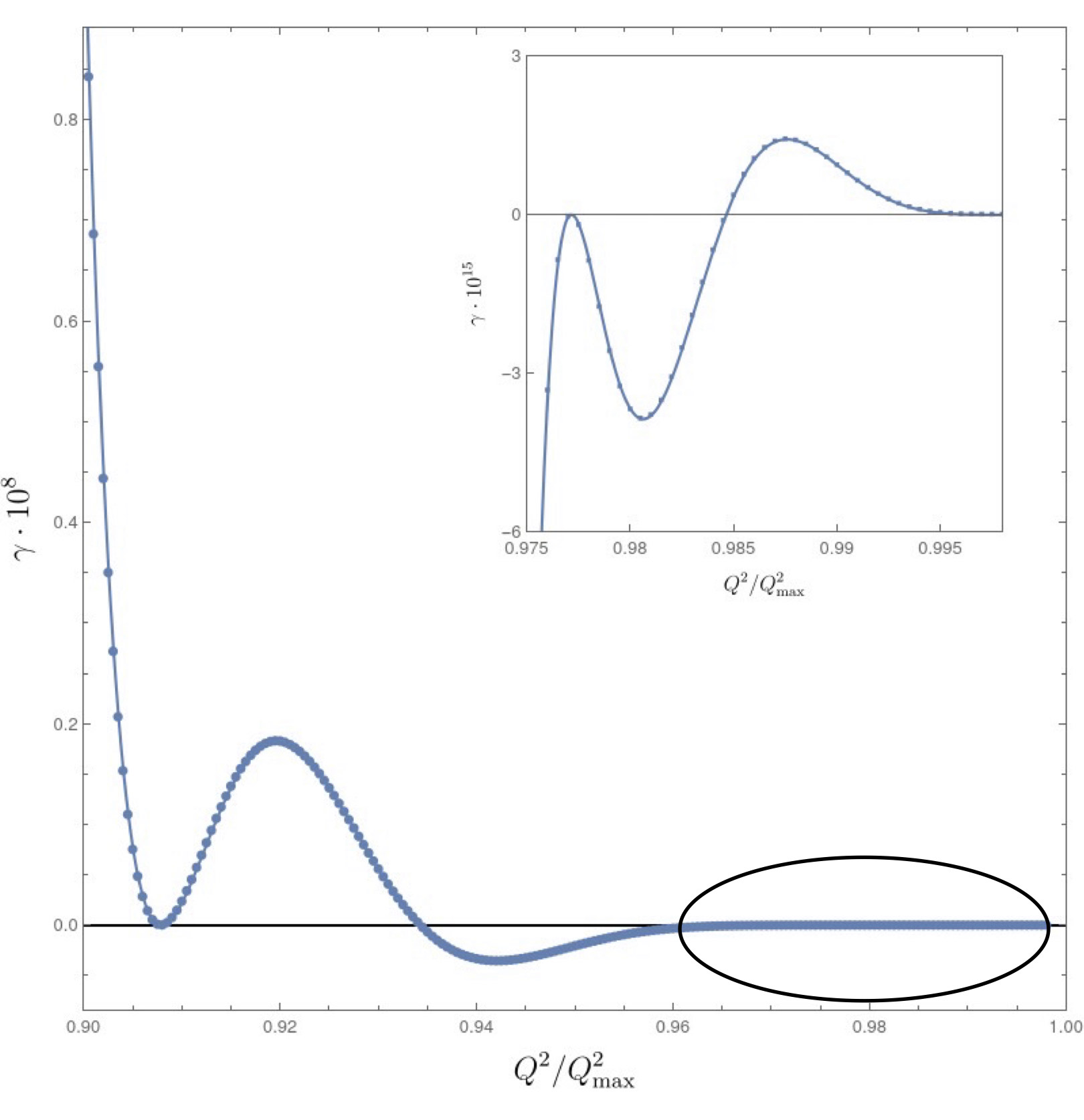
To obtain the spectrum of QNMs numerically we approximate the continuous ODE problem by a discrete system of equations, as seen in Dias et al. 2016; Dias et al. 2010; Trefethen 2000; Boyd et al. 2000. More specifically, we sample solutions of equation (42) in a discrete Chebyshev grid, mapping the differential operator into a matrix operator. We then solve the resulting matrix equation using standard linear algebra methods.

For a given interval $[a,\,b]$ we may define a Chebyshev grid with size $N_{c}$ as the set of points $x_{i}$ such that

$$x_{i}=\frac{(b-a)}{2}\cos\left(\frac{i\,\pi}{N_{c}}\right)\,+\,\frac{a+b}{2},\quad\quad i=0,\,1,\,2,\,...,\,N_{c}\quad.$$

(51)

Constraining the domain to the discrete Chebyshev grid, we may rewrite the action of the derivative using matrix multiplication. We denote this matrix $D_{c}$, (see Trefethen 2000 for an explicit definition). Multiplying equation (42) by $y(y-1)$ and sampling it in the Chebyshev grid above, we obtain a quadratic matrix eigenvalue problem. The eigenvectors will be discrete approximations of solutions to equation (42), smooth at $y\,=\,0$ and $y\,=\,1$. The eigenvalues will correspond to approximations of the Quasinormal Frequencies.

To find the frequencies we use a combination of two methods. We start by obtaining a direct eigenvector decomposition of the system using Mathematica’s native Eigensystem function. This method yields an approximation of the full frequency spectrum. Bear in mind it is very important to use a software that supports arbitrary precision to obtain good results (we used up to 500 digits of precision in intermediate calculations). This procedure, is not the best to approximate the frequency of individual modes. It is too computational intensive, and does not allow arbitrary high precision of a given frequency. Bearing this in mind, we apply the version of the Newton-Raphson method described in Dias et al. 2010; Dias et al. 2016; Tisseur and Meerbergen 2001 using the direct method as a seed. Although faster and more precise, this method requires a very accurate initial frequency estimate to converge. In figure 6, we plot the numerical error on the calculation of a given quasinormal frequency as a function of the Chebyshev grid size $(N_{c})$. As expected, we see that the usage of a Chebyshev grid actually guarantees that this method has exponential convergence.

In the analysis below, we computed the lowest lying NE exterior and type-b interior QNMs (see equation (50) for a definition) in a non-trivial region of the parameter space. To achieve this, we used the direct method to obtain these modes for a given RNdS BH, and then used them as seed for a Newton-Raphson method applied to BHs with similar mass and charge. We then used the results as estimates on other similar BHs and henceforth. For each frequency calculated, we repeated this procedure twice, once with a Chebyshev grid size of 500, and then 550. The difference between the obtained frequencies was used to estimate the precision of our calculations. We always made sure this was at least one order of magnitude below the difference between interior and exterior QNM frequencies. This limit would only saturate close to extremality, otherwise, the precision was usually much higher than the difference in frequencies.

As seen in section IV.2, in the NE limit of RNdS BHs, there is a correspondence between the spectrum of NE exterior modes and type-b interior modes. Using numerics, we verified whether this correspondence extends to the remainder of parameter space. To do so, we explicitly computed the lowest lying frequency of the NE family of exterior modes ($\omega_{\text{ext}}$) and the lowest lying frequency of type-b interior modes ($\omega_{\text{int}}$). To make sure we chose the appropriate families, we compared with the analytic prediction in the near extremal limit (equation (50)). We performed this calculation for $\Phi_{+}\,(l=1)$ and $\Phi_{-}\,(l=2)$ gravitoeletric QNMs in a large class of RNdS black holes.

In our plots, we characterize the difference using the quantity

$$\gamma=\left(\frac{\omega_{\text{in}}\,-\,\omega_{\text{ext}}}{\omega_{\text{in}}\,+\,\omega_{\text{ext}}}\right).$$

(52)

This will always be a real number, as the modes we are concerned with have purely imaginary frequency.

In figure 4 we plot $\gamma$ as a function of $Q^{2}/Q^{2}_{\text{max}}$ for a fixed value of $y_{+}$. Similarly, in figure 5, we depict $\gamma$ in a non-trivial region of parameter space using a density plot. We see that $\gamma$ oscillates around 0, attaining the value in some simple roots and occasional double roots (as seen in the beginning of figure 4(a)).

Analysing figure 5, we see $\gamma$ is always very small, reaching a maximum of $\mathcal{O}(10^{-6})$. Although the frequencies are very similar as expected, they are not equal. It is interesting to analyse the dark regions in 5. When the colour changes from purple to orange, we have single 0’s of $\gamma$, whereas when there is no colour change, we have double zeros, as seen above. In figure 7, we prove that this features are actually present, by zooming in around one of these roots. These features are unexpected as both the frequencies and their gradient coincide. Close to these lines, there is a wider region where $\gamma$ is close to 0. The roots of $\gamma$ are 1-dimensional regions of parameter space. For these black holes, fields will have increased regularity at the Cauchy horizon. Nevertheless, these regions are not generic in the 2-dimensional parameter space of RNdS BHs, so they are not pointers to SCC violations. Finally, it is worth remarking that $\gamma$ approaches 0 in the extremal limit, validating the discussion in section IV.2.

We can conclude that lowest lying exterior frequencies, generically, are not the frequencies of interior modes. Hence the regularity of gravitoelectromagnetic perturbations on a generic RNdS black hole, agree with the ones found in Dias et al. 2018a. Hence, there are no new violations of SCC.

As a toy example, we will focus in the behaviour of massless scalar fields in Kerr-dS spacetime. Our argument should be extendible to other fields without much difficulty. In the following, we will show that generic solutions of

$$\Box\Phi\,=\,0$$

(53)

do not have finite energy at the Cauchy horizon. We will take purely ingoing modes at the event horizon, with the frequency of an exterior mode, and scatter it through the BH interior, studying their regularity at the Cauchy horizon. In a Kerr-dS background, the radial and angular parts of the KG equation are given by the Teukolsky equation. Plugging (18) into (17), we obtain the following equations:

	$\displaystyle\begin{split}&{}\derivative{\theta}\left(\Delta_{\theta}\sin\theta\derivative{\Theta_{\omega l m}}{\theta}\right)\\ &{}-(m-a\omega\sin^{2}\theta)^{2}\frac{\Sigma^{2}}{\Delta_{\theta}\sin\theta}\Theta_{\omega lm}(\theta)\\ &{}+K_{lm}\sin(\theta)\Theta_{\omega lm}(\theta)\,=\,0\quad,\end{split}$			(54)
	$\displaystyle\begin{split}&\derivative{r}\left(\Delta_{r}\derivative{R_{\omega l m}(r)}{r}\right)\\ &+\left[\frac{\Sigma^{2}}{\Delta_{r}}(\omega(r^{2}+a^{2})-am)^{2}\,-\,K_{lm}\right]R_{\omega lm}(r)=0\quad,\end{split}$			(55)

here $m\in\mathbb{Z},\,|m|\leq l$ and $K_{lm}$ is the constant arising from separation of variables. For ease of notation we will henceforth drop the $\omega lm$ subscript.

Equation (55) has four regular singular points at the roots $r_{i}$ of $\Delta_{r}(r_{i})$. For $r>0$ this happens at the Cauchy horizon $(r_{-})$, the event horizon $(r_{+})$ and the Cosmological horizon $(r_{c})$. Solutions to this equation are defined in (20), (21) and (22).

The analysis of section III.2 tells us that for a QNM with

$$\frac{|Im(\omega)|}{\kappa_{-}}<\frac{1}{2}\quad,$$

(56)

$\Phi_{in,-}$ will have infinite energy at the Cauchy horizon. In Dias et al. 2018b, using a WKB analysis, it was proved that taking $l$ large enough we find modes respecting condition (56). We will now prove that for these modes the value of $\mathcal{A}(\omega)$ in equation (29) is non-zero, validating the conclusions of Dias et al. 2018b.

Below, we will study the continuation of an exterior QNM solution, onto the interior of the BH, and show that it has $\mathcal{A}(\omega)\neq 0$. To do so, we fix $K_{lm}$ and $\omega$ to the values obtained for WKB QNMs defined in Dias et al. 2018b. Exterior QNMs are purely ingoing at the event horizon. We use this to set the initial conditions for the wave function in the BH interior. Using a WKB approximation, we solve the radial equation, decomposing it in the $R_{in/out,-}$ basis, using equation (29).

Consider $r_{*}$ defined in (14), such that $r_{*}(r_{+})=+\infty$ and $r_{*}(r_{-})=-\infty$. In terms of $r_{*}$, the radial equation is

$$\derivative[2]{S}{r_*}\,+\,U(r,\omega,l,m)\,S(r)\,=\,0\quad,$$

(57)

where $S(r)\,=\,\sqrt{r^{2}+a^{2}}\,R(r)$, and

$$U=\left(\omega-\frac{am}{r^{2}+a^{2}}\right)^{2}-\frac{K_{lm}\,\Delta_{r}}{\Sigma^{2}(r^{2}+a^{2})^{2}}\\ +\,(r^{2}+a^{2})^{-4}\Bigg[-\Delta_{r}^{2}(r^{2}+a^{2})+3\Delta_{r}^{2}r^{2}\Bigg.\\ \Bigg.-r\Delta_{r}\,\derivative{\Delta_r}{r}\,(r^{2}+a^{2})\Bigg]\quad.$$

(58)

The modes studied in Dias et al. 2018b, are such that $m=l$. Using a WKB approximation, the authors show that in the large $l$ limit:

$$\omega=\omega_{R}+i\,\omega_{I}=l\,\Omega_{c}+\mathcal{O}(1)\quad,$$

(59)

here $\Omega_{c}$ is the rotation frequency of a photon propagating in the inner photon sphere, outside the black hole. This corresponds to $\Omega^{+}_{c}$ defined in equation (4.19) of Dias et al. 2018b. We expand $K_{ll}$ in powers of $l$:

$$K_{ll}\,=\,l^{2}\,\lambda_{-2}\,+\,l\,\lambda_{-1}\,+\,...$$

(60)

In appendix A, we prove that this expansion is valid and $\lambda_{-2}$ is real and positive. We can now define:

$$U_{0}=\left[\left(\Omega_{c}-\frac{a}{r^{2}+a^{2}}\right)^{2}-\frac{\,\lambda_{-2}\,\Delta_{r}}{\Sigma^{2}(r^{2}+a^{2})^{2}}\right]\quad,$$

(61)

so that

$$U=l^{2}U_{0}\,+\,\mathcal{O}(l)\quad\text{for}\quad l>>1\quad.$$

(62)

Notice that $U_{0}(r_{*})$ is a real function of $r_{*}$, whereas $U(r_{*})$ has non vanishing imaginary part. We explicitly verified, that for Kerr-dS BHs:

$$\Omega(r_{-})>\Omega_{c}>\Omega(r_{+})\quad,$$

(63)

where $\Omega(r)$ is defined in (16).

Using equations (63), (60) and the fact that $\Delta_{r}(r)<0$ in $r\in[r_{-},r_{+}]$, we can establish that $U_{0}(r_{*})>0$ in $r\in[r_{-},r_{+}]$. In the BH exterior $\Delta_{r}(r)>0$ and this is no longer the case.

We now solve equation (57) using a standard WKB expansion (see Bender and Orszag 1978):

$$S(r_{*})=\exp\left(\frac{1}{l}\sum_{n=0}^{\infty}\delta^{n}S_{n}(r_{*})\right).$$

(64)

Truncating to $n=1$, we obtain that in the large $l$ limit:

$$S(r_{*},\omega,l)=\sqrt{r^{2}+a^{2}}\,R_{in,+}\approx\\ U_{0}(r_{*})^{-\frac{1}{4}}\Bigg[A(\omega,l)\exp\left(il\int_{0}^{r_{*}}U_{0}(s)^{\frac{1}{2}}\differential s\right)\\ +B(\omega,l)\exp\left(-il\int_{0}^{r_{*}}U_{0}(s)^{\frac{1}{2}}\differential x\right)\Bigg]\quad,$$

(65)

where $A(\omega,l)$ and $B(\omega,l)$ are integration constants.

Given that $U_{0}(r_{*})>0$ everywhere, equation (65) is valid everywhere. Physically, this means that to leading order in $l$, there is no scattering of WKB modes propagating in the BH interior. However, to get $\mathcal{A}(\omega)=0$ we would need a purely ingoing mode at $\mathcal{H}^{+}$ to be fully scattered into an outgoing mode at $\mathcal{CH}_{R}$. Therefore we can already anticipate that no violations of SCC in the Kerr-dS spacetime will be found. Nevertheless, lets explicitly check this below.

For ease of notation, define

$$\omega_{+}=\omega-l\,\Omega_{+}\quad,\quad\omega_{-}=\omega-l\,\Omega_{-}\quad.$$

(66)

For $r_{*}\to-\infty$ (near $\mathcal{H}_{+}$), using equations (58) and (59), we obtain:

$$\lim_{r_{*}\to-\infty}\int_{0}^{r_{*}}\left(l\sqrt{U_{0}}-\omega_{+}\right)\,=\,\alpha_{+}\,l\quad,$$

(67)

where $\alpha_{+}=\mathcal{O}(1)$ as $l\to\infty$. Similarly, for $r_{*}\to\infty$ (near $\mathcal{CH}_{+}$), we get

$$\lim_{r_{*}\to\infty}\int_{0}^{r_{*}}\left(l\sqrt{U_{0}}-\omega_{-}\right)\,=\,\alpha_{-}\,l\quad.$$

(68)

Dropping the finite term $\sqrt{r^{2}+a^{2}}$ in front of $R(r)$, we find that near $\mathcal{H}_{+}$,

$$R(r_{*})\sim\left(\frac{\omega_{+}}{l}\right)^{-\frac{1}{4}}\Bigg[A(\omega,l)e^{-i\left(\omega_{+}r_{*}\,+\,\alpha_{+}l\right)}\\ +B(\omega,l)e^{i\left(\omega_{+}r_{*}\alpha\,+\,l\right)}\Bigg]\quad\text{as}\quad r_{*}\rightarrow-\infty\quad.$$

(69)

Similarly, at $\mathcal{CH}_{R}^{+}$, we get:

$$R(r_{*})\sim\left(\frac{\omega_{-}}{l}\right)^{-\frac{1}{4}}\Bigg[A(\omega,l)e^{-i\left(\omega_{-}r_{*}\,+\,\alpha_{-}l\right)}\\ +B(\omega,l)e^{i\left(\omega_{-}r_{*}\,+\,\alpha_{-}l\right)}\Bigg]\quad\text{as}\quad r_{*}\rightarrow\infty\quad.$$

(70)

Now, we take $R(r_{*})$ to be $R_{in,+}$. The ingoing condition (equation (21)) at $\mathcal{H}_{+}$ yields $R_{in,+}(r_{*})\sim e^{-i\omega_{+}r_{*}}$ as $r_{*}\rightarrow\infty$. This gives:

	$\displaystyle B(\omega,l)$	$\displaystyle\sim\mathcal{O}(l^{-1})\quad,$		(71)
	$\displaystyle A(\omega,l)$	$\displaystyle\sim\mathcal{O}(1)\quad.$		(72)

Now, focusing in the behaviour near $\mathcal{CH}_{R}^{+}$, using equation (29), we obtain:

	$\displaystyle\mathcal{A}(\omega)$	$\displaystyle=\left(\frac{\omega_{-}}{l}\right)^{-\frac{1}{4}}A(\omega,l)e^{-i\,\alpha_{-}l}\quad,$		(73)
	$\displaystyle\mathcal{B}(\omega)$	$\displaystyle=\left(\frac{\omega_{-}}{l}\right)^{-\frac{1}{4}}B(\omega,l)e^{i\,\alpha_{-}l}\quad,$		(74)

where

$$\frac{\omega_{-}}{l}=\mathcal{O}(1)\quad.$$

(75)

In particular, in large $l$ limit, $\mathcal{B}$ vanishes, so $\mathcal{A}(\omega)$ must be non zero, or we would have the trivial solution. Hence, we prove that $\mathcal{A}(\omega)\neq 0$ for $\omega$ a QMN frequency. The conclusion of Dias et al. 2018b is maintained, preserving SCC for the Kerr-dS BH.

References

- Penrose (1978) R. Penrose, Singularities of spacetime., in Theoretical Principles in Astrophysics and Relativity, edited by N. R. Lebovitz (1978) pp. 217–243.
- Simpson and Penrose (1973) M. Simpson and R. Penrose, Internal instability in a Reissner-Nordstrom black hole, Int. J. Theor. Phys. 7, 183 (1973).
- McNamara (1978) J. M. McNamara, Instability of black hole inner horizons, Proceedings of the Royal Society of London. Series A, Mathematical and Physical Sciences 358, 499 (1978).
- Chandrasekhar and Hartle (1982) S. Chandrasekhar and J. B. Hartle, On crossing the cauchy horizon of a reissner-nordstrom black-hole, Proceedings of the Royal Society of London. Series A, Mathematical and Physical Sciences 384, 301 (1982).
- Poisson and Israel (1990) E. Poisson and W. Israel, Internal structure of black holes, Phys. Rev. D 41, 1796 (1990).
- Dafermos (2005) M. Dafermos, The interior of charged black holes and the problem of uniqueness in general relativity, Communications on Pure and Applied Mathematics 58, 445 (2005), https://onlinelibrary.wiley.com/doi/pdf/10.1002/cpa.20071 .
- Dafermos and Shlapentokh-Rothman (2017) M. Dafermos and Y. Shlapentokh-Rothman, Time-Translation Invariance of Scattering Maps and Blue-Shift Instabilities on Kerr Black Hole Spacetimes, Commun. Math. Phys. 350, 985 (2017), arXiv:1512.08260 [gr-qc] .
- Luk and Oh (2017) J. Luk and S.-J. Oh, Proof of linear instability of the Reissner–Nordström Cauchy horizon under scalar perturbations, Duke Math. J. 166, 437 (2017), arXiv:1501.04598 [gr-qc] .
- Mellor and Moss (1990) F. Mellor and I. Moss, Stability of Black Holes in De Sitter Space, Phys. Rev. D 41, 403 (1990).
- Cardoso et al. (2018a) V. Cardoso, J. a. L. Costa, K. Destounis, P. Hintz, and A. Jansen, Quasinormal modes and Strong Cosmic Censorship, Phys. Rev. Lett. 120, 031103 (2018a), arXiv:1711.10502 [gr-qc] .
- Hintz and Vasy (2017) P. Hintz and A. Vasy, Analysis of linear waves near the Cauchy horizon of cosmological black holes, J. Math. Phys. 58, 081509 (2017), arXiv:1512.08004 [math.AP] .
- Costa and Franzen (2017) J. a. L. Costa and A. T. Franzen, Bounded energy waves on the black hole interior of Reissner-Nordstr\”om-de Sitter, Annales Henri Poincare 18, 3371 (2017), arXiv:1607.01018 [gr-qc] .
- Cardoso et al. (2018b) V. Cardoso, J. L. Costa, K. Destounis, P. Hintz, and A. Jansen, Strong cosmic censorship in charged black-hole spacetimes: still subtle, Phys. Rev. D 98, 104007 (2018b), arXiv:1808.03631 [gr-qc] .
- Hintz (2016) P. Hintz, Non-linear stability of the Kerr-Newman-de Sitter family of charged black holes 10.1007/s40818-018-0047-y (2016), arXiv:1612.04489 [math.AP] .
- Hintz and Vasy (2016) P. Hintz and A. Vasy, The global non-linear stability of the Kerr-de Sitter family of black holes 10.4310/acta.2018.v220.n1.a1 (2016), arXiv:1606.04014 [math.DG] .
- Costa et al. (2018) J. a. L. Costa, P. M. Girão, J. Natário, and J. D. Silva, On the Occurrence of Mass Inflation for the Einstein–Maxwell-Scalar Field System with a Cosmological Constant and an Exponential Price Law, Commun. Math. Phys. 361, 289 (2018), arXiv:1707.08975 [gr-qc] .
- Dias et al. (2018a) O. J. Dias, H. S. Reall, and J. E. Santos, Strong cosmic censorship: taking the rough with the smooth, JHEP 10, 001, arXiv:1808.02895 [gr-qc] .
- Dias et al. (2019a) O. J. Dias, H. S. Reall, and J. E. Santos, Strong cosmic censorship for charged de Sitter black holes with a charged scalar field, Class. Quant. Grav. 36, 045005 (2019a), arXiv:1808.04832 [gr-qc] .
- Dias et al. (2018b) O. J. Dias, F. C. Eperon, H. S. Reall, and J. E. Santos, Strong cosmic censorship in de Sitter space, Phys. Rev. D 97, 104060 (2018b), arXiv:1801.09694 [gr-qc] .
- Dias et al. (2019b) O. J. Dias, H. S. Reall, and J. E. Santos, The BTZ black hole violates strong cosmic censorship, JHEP 12, 097, arXiv:1906.08265 [hep-th] .
- Banados et al. (1992) M. Banados, C. Teitelboim, and J. Zanelli, The Black hole in three-dimensional space-time, Phys. Rev. Lett. 69, 1849 (1992), arXiv:hep-th/9204099 .
- Dafermos and Shlapentokh-Rothman (2018) M. Dafermos and Y. Shlapentokh-Rothman, Rough initial data and the strength of the blue-shift instability on cosmological black holes with , Class. Quant. Grav. 35, 195010 (2018), arXiv:1805.08764 [gr-qc] .
- Hollands et al. (2020a) S. Hollands, R. M. Wald, and J. Zahn, Quantum instability of the cauchy horizon in reissner–nordström–desitter spacetime, Classical and Quantum Gravity 37, 115009 (2020a).
- Hollands et al. (2020b) S. Hollands, C. Klein, and J. Zahn, Quantum stress tensor at the Cauchy horizon of the Reissner–Nordström–de Sitter spacetime, Phys. Rev. D 102, 085004 (2020b), arXiv:2006.10991 [gr-qc] .
- Emparan and Tomašević (2020) R. Emparan and M. Tomašević, Strong cosmic censorship in the BTZ black hole, JHEP 06, 038, arXiv:2002.02083 [hep-th] .
- Wald (1984) R. M. Wald, General Relativity (Chicago Univ. Pr., Chicago, USA, 1984).
- Berti et al. (2009) E. Berti, V. Cardoso, and A. O. Starinets, Quasinormal modes of black holes and black branes, Classical and Quantum Gravity 26, 163001 (2009).
- Kokkotas and Schmidt (1999) K. D. Kokkotas and B. G. Schmidt, Quasinormal modes of stars and black holes, Living Rev. Rel. 2, 2 (1999), arXiv:gr-qc/9909058 .
- Moitra (2020) U. Moitra, On Strong Cosmic Censorship in Two Dimensions, (2020), arXiv:2011.03499 [hep-th] .
- Bender and Orszag (1978) C. Bender and S. Orszag, Advanced Mathematical Methods for Scientists and Engineers I: Asymptotic Methods and Perturbation Theory (1978).
- Kristensson (2010) G. Kristensson, Second order differential equations. Special functions and their classification (2010).
- Dias et al. (2016) O. J. Dias, J. E. Santos, and B. Way, Numerical Methods for Finding Stationary Gravitational Solutions, Class. Quant. Grav. 33, 133001 (2016), arXiv:1510.02804 [hep-th] .
- Dias et al. (2010) O. J. Dias, P. Figueras, R. Monteiro, H. S. Reall, and J. E. Santos, An instability of higher-dimensional rotating black holes, JHEP 05, 076, arXiv:1001.4527 [hep-th] .
- Trefethen (2000) L. N. Trefethen, Spectral Methods in MatLab (Society for Industrial and Applied Mathematics, USA, 2000).
- Boyd et al. (2000) J. Boyd, T. Marilyn, and P. Eliot, Chebyshev and fourier spectral methods, (2000).
- Tisseur and Meerbergen (2001) F. Tisseur and K. Meerbergen, The quadratic eigenvalue problem, SIAM Review 43, 235 (2001).