We are interested in the case that both of dark matter $\chi$ and the CP-even scalar $\phi$ ($\simeq h_{2}$) are never thermalized with the SM particles. This is achieved by tiny values of quartic couplings $\lambda_{H\Phi}$ and $\lambda_{\Phi}$, roughly speaking, $\lambda_{H\Phi},\lambda_{\Phi}\lesssim 10^{-6}$. From the theoretical side, a radiative correction to the $|\Phi|^{4}$ term would imply its lower bound, $\lambda_{\Phi}\gtrsim\lambda_{H\Phi}^{2}/16\pi^{2}$. With these feeble couplings, both of $\phi$ and $\chi$ become the FIMPs, and the Boltzmann equations for the number densities $n_{\phi}$ and $n_{\chi}$ are given by

where $C_{A\leftrightarrow B}$ in the right-hand side denotes the collision term corresponding to the process $A\leftrightarrow B$. Here the broken phase of $\Phi$ is assumed and the scalars in the dark sector interact with the SM only through the Higgs doublet. The explicit form of collision terms is

where $f_{x}$ is the distribution function of particle $x$, $d\Pi_{x}$ is the Lorentz-invariant phase space expressed as $d\Pi_{x}=\frac{d^{3}\bm{p}_{x}}{(2\pi)^{3}2E_{\bm{p}_{x}}}$, and $\mathcal{M}_{X}$ denotes the amplitude of the process $X$.

Since dark matter is produced by the freeze-in mechanism from the SM thermal bath, the magnitude of distribution functions is tiny for $\phi$ and $\chi$. Thus the $\mathcal{O}(f_{\phi,\chi}^{2})$ terms can be dropped in the above equations. This approximation is valid as long as the distribution functions $f_{\phi,\chi}$ are not close to the equilibrium one before the abundance is frozen. The Boltzmann equations are thus reduced to

where the decay widths are given by

Note that we have used the relation $m_{\phi}^{2}=\lambda_{\Phi}v_{\phi}^{2}$ in the above equations and the SM Higgs doublet contains real four components, leading to the difference of numerical factors. The mass parameter $m_{H}$ for the $H$ field will be discussed in the next section. Introducing the net dark matter number density $n_{D}=n_{\chi}+2\mathrm{Br}^{\phi\to\chi\chi}n_{\phi}$, the Boltzmann equation for $n_{D}$ is recast as

where $\mathrm{Br}^{\phi\to\chi\chi}$ is the branching ratio defined by $\mathrm{Br}^{\phi\to\chi\chi}=\Gamma_{\phi\to\chi\chi}/(\Gamma_{\phi\to H^{\dagger}H}+\Gamma_{\phi\to\chi\chi})$. The collision terms are written by using the thermally averaged cross sections and the number density of the SM Higgs doublet in thermal bath, $n_{H}^{\mathrm{eq}}$. Then we obtain

The first term in the right-hand side denotes the dark matter production directly from the thermal bath, and the second and third terms are the contributions from the decays of $\phi$ produced from the thermal bath. The thermally averaged cross sections are explicitly calculated as

where we have defined the integral variable $z\equiv\sqrt{s}/T$ for the Mandelstam $s$ variable, the dimensionless parameters $x_{i}\equiv m_{i}/T$ and $\gamma_{i}\equiv\Gamma_{i}/T$ for a particle $i$ with the mass $m_{i}$ and the total decay width $\Gamma_{i}$. In the integrals, the lower limits are given by $\bar{x}_{\chi,\phi}=\max[x_{\chi,\phi},x_{H}]$ and $K_{1}(z)$ is the modified Bessel function of second kind of order 1. Here thermal bath particles are assumed to obey the Maxwell-Boltzmann distribution.¹¹ 1 Quantum statistical distributions may give a small factor difference in numerical calculations [18]. Note that the integrand in Eq. (3.10) contains the factor $z^{4}$ due to the derivative coupling of pNGB dark matter. This behavior implies that even if the portal coupling $\lambda_{H\Phi}$ is large, the dark matter reaction rate with the SM is suppressed in lower energy than $m_{\phi}$ and the usual freeze-out does not work in the case of the hierarchical VEV $v_{\phi}\gg v\,$ ($m_{\phi}\gg m_{h}$).

The one-loop effect of bath particles leads to the mass corrections quadratically scaling by the temperature, which are called thermal masses. Including thermal mass corrections gives important effects for collision terms (reaction rates) and hence for the evaluation of relic abundance of dark matter. The detailed calculation of thermal mass for the SM Higgs boson is summarized in Appendix A. The electroweak gauge bosons, all SM fermions, and all components of $H$ including the NGBs eaten by the gauge bosons contribute to the thermal mass, which is given by

where $g_{Y}$ and $g_{2}$ are the gauge couplings of $U(1)_{Y}$ and $SU(2)_{L}$, and $y_{t}$ is the top Yukawa coupling which is dominant over the other Yukawa couplings. Including this thermal contribution, the mass of the SM Higgs boson is given by

which plays a role of regulator in the reaction rates in the Boltzmann equations.

When the reheating temperature of the universe, $T_{R}$, is higher than the heavy mediator mass $m_{\phi}$, the final abundance of dark matter is determined independently of the reheating temperature. This is so-called the IR freeze-in [15]. The analytic formula of the dark matter yield $Y_{D}=n_{D}/s$ derived from Eq. (3.9) is approximately given by

The result is found to be independent of the dark matter mass because the dominant production process comes from the $\phi$ decay around $T\sim m_{\phi}$, as shown in the following part. In the limit where the scalar VEV and the mass of $\phi$ are much larger than the masses of the SM Higgs boson and dark matter, the factor of quartic couplings $\mathrm{Br}^{\phi\to\chi\chi}\lambda_{H\Phi}^{2}$ reduces to

Thus combining the IR freeze-in relic Eq. (3.15) and the yield corresponding to the observed value $Y_{D}^{\mathrm{obs.}}=4.4\times 10^{-7}\left(m_{\chi}/\rm{MeV}\right)^{-1}$ [16] with $g_{*}\sim g_{*}^{S}\sim 100$, we obtain the following relations

The evolution of the reaction rates including the thermal mass effects is shown in the left panel of Fig. 1 where we choose the following parameter set

as a benchmark. This is chosen so that the parameter relation Eq. (3.18) is realized. Note that the portal coupling should satisfy $\lambda_{H\Phi}\lesssim 10^{-6}$ in order for the dark sector particles not to enter into the thermal bath. When the temperature cools down to the mediator mass scale $T\sim m_{\phi}$, a number of on-shell $\phi$ are resonantly produced. As a result the magnitude of the reaction rate for the process $H^{{\dagger}}H\to\chi\chi$ rapidly increases as can be seen in Fig. 1.

For the same benchmark parameter set, the evolution of the dark matter yield is shown in the right panel of Fig. 1, assuming the vanishing initial conditions of the dark sector

We also show for comparison the results calculated by the public code MicrOMEGAs [19] with and without the thermal mass effect for the SM Higgs boson.²² 2 In the current version of MicrOMEGAs, full thermal mass effects are not implemented. However it is possible to include the thermal mass only for the Higgs boson by hand without difficulty. As obvious from the plot, the thermal mass effect gives an impact on the evolution of the dark matter yield, in particular when the temperature is $T\gtrsim m_{\phi}$. Including thermal mass also affects the final dark matter abundance, while its impact is not so large and only gives a few factor difference. One can see from the plot that the yield of dark matter rapidly grows at $T\sim m_{\phi}$ due to the resonant production of $\phi$, and then the evolution is almost frozen afterwards.

The purple and red lines in the left panel of Fig. 2 show the contours in the ($m_{\chi}$, $\lambda_{\Phi}$) plane reproducing the dark matter relic abundance observed by the PLANCK Collaboration [16]. The reheating temperature is assumed to be much higher than the mediator mass scale ($T_{R}\gg m_{\phi}$). As can be seen in the plots, for a larger $m_{\phi}$ the lines simply shift to the right (purple to red), namely the direction of heavier dark matter mass which compensates a smaller yield $Y_{D}^{\mathrm{IR}}$. The behavior of the lines change around $\lambda_{\Phi}\sim\lambda_{H\Phi}$ as explained in Eqs. (3.17) and (3.18). While one can take a heavier dark matter mass $m_{\chi}$ if a larger mediator mass $m_{\phi}$ is chosen, there is an upper bound on $m_{\chi}$ if the criterion for the VEV $v_{\phi}<M_{P}$ is taken into account. As we will discuss in the next section, a feeble value of the scalar self-coupling, typically $\lambda_{\Phi}\gtrsim\mathcal{O}(10^{-12})$ is suitable for $\phi$ being the inflaton.

When $m_{\phi}$ is much larger than the reheating temperature, the dark matter relic abundance is determined by the portal coupling $\lambda_{H\Phi}$ and the reheating temperature $T_{R}$. This is so called the UV freeze-in discussed in Refs. [15, 20]. For $T<T_{R}\ll m_{\phi}$, only the $H^{{\dagger}}H\to\chi\chi$ process is effective for the dark matter production (see the left panel of Fig. 1). In the $H^{{\dagger}}H\to\chi\chi$ reaction rate (3.10), we can safely assume $m_{\phi}\gg\sqrt{s}\gg m_{h},m_{\chi}$ since the modified Bessel function regarded as the window function with a cut-off $T$ and the large $s$ contribution is dominant due to the $s^{5/2}$ behavior of the integrand. Thus the reaction rate is approximated by

By integrating the Boltzmann equations for the dark sector using this approximation, the pNGB dark matter yield is evaluated as

Combining with the observed value $Y_{D}^{\mathrm{obs.}}=4.4\times 10^{-7}\left(m_{\chi}/\rm{MeV}\right)^{-1}$ with $g_{*}\sim g_{*}^{S}\sim 100$, we obtain the following relation³³ 3 For a heavier pNGB dark matter case, the broader parameter space in the $(m_{\phi},\lambda_{H\Phi})$ plane has been discussed in Ref. [21].

The right panel of Fig. 2 shows the parameter space where the dark matter relic can be realized by the UV freeze-in, which is denoted by the purple region. The purple solid, dashed and dot-dashed lines denote $m_{\phi}=100\,T_{R}$, $10\,T_{R}$ and $T_{R}$ (the UV freeze-in (3.22) is valid for $m_{\phi}\gg T_{R}$). The red lines show the contours in the $(m_{\chi},\lambda_{H\Phi})$ plane reproducing the dark matter relic for various given reheating temperatures. Note that the green colored region $m_{\phi}\geq 10^{-3}M_{P}$ is excluded by the conditions $v_{\phi}\leq M_{P}$ and $\lambda_{\Phi}\leq 10^{-6}$, the latter of which is required for the dark sector not being thermalized.

The inflation gives a plausible solution for the flatness and horizon problems in the universe. A successful inflation scenario can occur in our model if a non-minimal coupling between the complex scalar $\Phi$ and gravity is introduced. Then the Lagrangian relevant for the inflation dynamics is given by

where $\mathcal{R}$ is the Ricci scalar and $\xi$ is the so-called non-minimal coupling constant. During the inflation era, the scalar potential is assumed to be dominated by the field value of $\Phi$, thus $\mathcal{V}(\Phi)\approx\lambda_{\Phi}|\Phi|^{4}/2\approx\lambda_{\Phi}\phi^{4}/8$, and the $|\Phi|^{2}$ part can be written as $|\Phi|^{2}\approx\phi^{2}/2$ with the non-linear representation $\Phi=\left(v_{\phi}+\phi\right)e^{i\chi/v_{\phi}}/\sqrt{2}$.

The non-minimal coupling is removed by the conformal transformation,

where $\hat{g}_{\mu\nu}$ corresponds to the metric in the Einstein frame. As a result of this transformation, the Lagrangian becomes

where $\varphi$ and $\hat{\chi}$ are the canonically normalized fields satisfying the differential equations

If $\xi\gg 1$, which is similar to the case of the Higgs inflation [24], the differential equation is simplified and the explicit expressions of $\varphi$ and $\hat{\mathcal{V}}(\varphi)$ are obtained. However in the present pNGB model with feeble couplings, we will show later that a smaller $\xi$ is favored for successful inflation. The shape of the scalar potential is numerically evaluated and shown in Fig. 3 where the non-minimal coupling is fixed to be $\xi=10^{-2},10^{-1},1$. The flat part of the potential gets longer for a smaller value of $\xi$.

While one cannot write down the explicit form of the scalar potential $\hat{\mathcal{V}}(\varphi)$, the slow-roll parameters are expressed in terms of $\phi$,

where $\hat{\mathcal{V}}_{\varphi}\equiv\partial\hat{\mathcal{V}}/\partial\varphi$ and $\hat{\mathcal{V}}_{\varphi\varphi}\equiv\partial^{2}\hat{\mathcal{V}}/\partial\varphi^{2}$. Using the slow-roll approximation, the spectral index $n_{s}$ and the tensor-to-scalar ratio $r$ are given by

The e-folding number $N_{*}$ between the time of horizon exit ($t_{*}$) and the end of inflation ($t_{\mathrm{end}}$) is given by

where $\phi_{*}$ and $\phi_{\mathrm{end}}$ are the field values at $t_{*}$ and $t_{\mathrm{end}}$, respectively. Defining $t_{\mathrm{end}}$ as the time giving the slow-roll parameter $\epsilon=1$ in Eq. (4.5), $\phi_{\mathrm{end}}$ satisfies

On the other hand, $\phi_{*}$ is numerically evaluated, giving the amplitude of the scalar power spectrum at the horizon exit observed by the Planck Collaboration [25]: $A_{s}=\hat{\mathcal{V}}(\varphi(\phi_{*}))/\left(24\pi^{2}M_{P}^{4}\,\epsilon(\phi_{*})\right)=2.10\times 10^{-9}$. From these relations, the non-minimal coupling $\xi$ and the scalar self-coupling $\lambda_{\Phi}$ for successful inflation can be read. The contour of the e-folding number $N_{*}$ on the ($\xi$, $\lambda_{\Phi}$) plane is shown in the left panel of Fig. 4 where $N_{*}=50$ and $60$. When the non-minimal coupling $\xi$ is small enough ($\xi\lesssim 10^{-3}$), the dependence on $\lambda_{\Phi}$ disappears. This region has the same behavior as the $\phi^{4}$ chaotic inflation.

The predictions for the spectral index $n_{s}$ and the tensor-to-scalar ratio $r$ at the pivot scale $k_{*}=0.002~\mathrm{Mpc}^{-1}$ are shown in the right panel of Fig. 4 where $N_{*}$ is taken to be between $50$ and $60$. The blue and light blue regions represent the $1\sigma$ and $2\sigma$ confidence levels observed by the Planck Collaboration [25]. It can be found that the lower bounds for the non-minimal coupling are required

for the scenario consistent with the observation.

In the left panel of Fig. 4, the solid (dotted) part of each contour represents the parameter region consistent (inconsistent) with the PLANCK observation at $2\sigma$ confidence level, when combined with the lower bounds of $\xi$ obtained in the right panel. We find that the self-coupling $\lambda_{\Phi}$ should be in the range $\lambda_{\Phi}\gtrsim 10^{-12}$ in the pNGB dark matter model with large symmetry breaking, if the inflation is induced by the coupling $\xi$.

There is another important physical implication of the possibility that the radial scalar component $\phi$ plays the role of inflaton in the pNGB dark matter model. That is the direct production process of dark matter $\chi$ from the inflaton decay, which is inevitable because of the interaction between $\phi$ and $\chi$. In this section, we investigate the parameter space consistent with the inflationary scenario discussed above and the dark matter relic abundance taking into account both the freeze-in and inflaton-induced dark matter.

As discussed in Refs. [26, 27], the number density of the inflaton induced $\chi$ particle is estimated as

where $\rho_{\rm rh}$ and $H(T_{R})$ are the energy density of radiation and the Hubble rate at the reheating temperature $T_{R}$. We here define the reheating temperature $T_{R}$ at which the Hubble rate is equal to the decay width of the inflaton to the SM sector ($H(T_{R})\approx\Gamma_{\phi\to H^{{\dagger}}H}$), and then

Note that the effective degrees of freedom $g_{*}$ in the right-hand side also depends on the temperature in general. Using the explicit form of the decay widths and the reheating temperature (4.12), we obtain the pNGB dark matter yield directly produced from the inflaton as

As previously, we impose the portal coupling satisfies $\lambda_{H\Phi}\lesssim 10^{-6}$ such that dark matter does not get into the SM thermal bath.

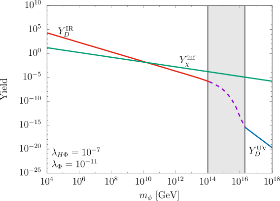
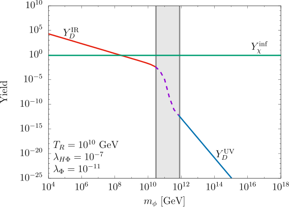
We here comment on the comparison between the three contributions of pNGB dark matter yields, $Y^{\mathrm{IR}}_{D}$, $Y^{\mathrm{UV}}_{D}$ and $Y^{\mathrm{inf}}_{\chi}$. Typical behaviors are shown in Fig. 5 as the functions of the mediator mass $m_{\phi}$, which behaviors are evaluated by MicrOMEGAs for $\lambda_{H\Phi}=10^{-7}$ and $10^{-11}$. The reheating temperature is given by Eq. (4.12) in the left panel, while it is treated as a free parameter in the right panel (see the detail in the next subsection). The IR and UV freeze-in productions are effective in the smaller and larger $m_{\phi}$ regions, respectively. These freeze-in yields are smoothly connected in the gray region where $T_{R}\lesssim m_{\phi}\lesssim 100\,T_{R}$, which is denoted by the purple dashed line. Since $Y^{\mathrm{IR}}_{D}\propto m_{\phi}^{-1}$ and $Y^{\mathrm{inf}}_{\chi}\propto m_{\phi}^{-1/2}$, the IR freeze-in is dominant for a lighter mediator. Further, $Y^{\mathrm{IR}}_{D}$ becomes equal to $Y^{\mathrm{inf}}_{\chi}$ at $m_{\phi}=m_{\mathrm{eq}}$. It is easy to find from Eqs. (3.15), (4.12) and (4.13) that $m_{\mathrm{eq}}\lesssim 10^{-2}\,T_{R}$, and then the inflaton-induced yield necessarily becomes dominant in the left side of the gray band. On the other hand, the UV freeze-in abundance takes the value $Y^{\mathrm{UV}}_{D}/Y^{\mathrm{inf}}_{\chi}\simeq 10^{-3}\lambda_{H\Phi}^{2}/\lambda_{\Phi}$ around $m_{\phi}=T_{R}$. This ratio is much smaller than 1 due to the constraints $\lambda_{H\Phi}\lesssim 10^{-6}$ and $\lambda_{\Phi}\gtrsim 10^{-12}$ as we explained from the cosmological arguments. Since $Y^{\mathrm{UV}}_{D}\propto m_{\phi}^{-5/2}$, the UV freeze-in contribution is always subdominant compared to the inflaton decay.

Fig. 6 shows the parameter space realizing the correct dark matter relic abundance in the $(m_{\chi},\lambda_{\Phi})$ plane taking into account the pNGB production from the freeze-in and inflaton decay. The portal coupling is chosen as $\lambda_{H\Phi}=10^{-7}$, $10^{-8}$ and $10^{-9}$ and the mediator mass is $m_{\phi}=10^{4}~\mathrm{GeV}$, $10^{6}~\mathrm{GeV}$ and $10^{8}~\mathrm{GeV}$. The purple line represents the parameters reproducing the dark matter abundance only by the freeze-in contribution. The gray region represents the parameter space where the inflaton induced dark matter abundance is larger than $10~\%$ of the observed value. In order to be consistent with the inflation observables at $2\sigma$ confidence level as discussed in the previous subsection, the scalar self-coupling has to satisfy $\lambda_{\Phi}\gtrsim 10^{-12}$ and the lower orange region is excluded by this condition.

The behavior of the purple lines in the most of panels can be understood by the IR freeze-in as discussed in Sec. 3.3, except the right-bottom one. The region $\lambda_{\Phi}\gtrsim 10^{-9}$ of that plot corresponds to the intermediate state between the IR and UV freeze-in, namely $T_{R}\sim m_{\phi}$, while the contribution to the relic from the inflaton decay is eventually dominant in this region. In case that the reheating temperature determined by the inflaton decay is much lower than the mediator mass $m_{\phi}$, since the reheating temperature scales as $T_{R}\propto\lambda_{H\Phi}\lambda_{\Phi}^{-1/2}m_{\phi}^{1/2}$ which can be seen in Eq. (4.12), it finds that the self-coupling goes as $\lambda_{\Phi}\propto m_{\chi}^{2/3}$ to reproduce the correct relic abundance from Eq. (3.23) for the UV freeze-in. This behavior has been numerically checked in our computation.

Fig. 7 shows the parameter space in the $(m_{\chi},\lambda_{\Phi})$ plane realizing the correct dark matter relic abundance via both contributions from the freeze-in and inflaton induced productions. The red and blue regions mean the abundance is dominated by the freeze-in and the inflaton, respectively. The red dot-dashed line denotes $m_{\phi}=T_{R}$. In the green region, the singlet scalar VEV ($v_{\phi}$) becomes trans-Planckian, where the low-energy field description is not valid.⁵⁵ 5 When one considers graviton loop effect, its form may be $\frac{m^{2}}{16\pi^{2}M_{P}^{2}}$ where $m$ is a typical scale in low-energy theory. Therefore the low-energy perturbative description is violated above $m_{P}\simeq 4\pi M_{P}$. If one imposes the condition $v_{\phi}<m_{P}$ in Fig. 7, the green excluded region is relaxed by $4\pi$. When the dark sector scalars $\phi$ and/or $\chi$ are heavy, the inflaton decay tends to be the dominant process for the dark matter creation. A physical implication of Fig. 7 is that in the pNGB dark matter model with large symmetry breaking, the dark matter should be lighter than MeV--GeV if the freeze-in production is assumed to be dominant.⁶⁶ 6 The light dark matter is constrained from the dark matter free streaming length being inconsistent with measurements of the Lyman-alpha forest [28, 29]. This typically excludes the dark matter mass region lighter than keV, which gives the lower mass bound. A heavier dark matter is also possible if taking the inflaton induced contribution into account.

In the above analysis, we have assumed that the reheating of the universe simply occurs via the inflaton perturbative decay to the Higgs field. However if there exists some other decay modes of the inflaton, the reheating temperature generally takes a different value. In this situation, the inflaton induced dark matter is estimated by

which is independent of the Higgs portal coupling $\lambda_{H\Phi}$ and almost independent of $m_{\phi}$ for a relatively heavy $\phi$. The pNGB abundance from the UV freeze-in is also implicitly changed since the parameter dependence of $T_{R}$ is modified from Eq. (4.12) to a free parameter, though the formula of $Y_{D}^{\mathrm{UV}}$ is still valid. In the same fashion in Fig. 7, we draw the parameter space realizing the correct dark matter abundance via both of freeze-in and inflaton decay (Fig. 8). We find in almost all allowed regions the freeze-in production is dominant. This comes from the fact that the inflaton induced abundance Eq. (4.14) is almost insensitive to $m_{\phi}$. Compared with Fig. 7, a heavier dark matter is possible up to $\mathcal{O}(10-100)~\mathrm{GeV}$ with a higher reheating temperature.

References

- [1] E. Aprile et al. [XENON], Phys. Rev. Lett. 121 (2018) no.11, 111302 [arXiv:1805.12562 [astro-ph.CO]].
- [2] E. Aprile et al. [XENON], JCAP 11 (2020), 031 [arXiv:2007.08796 [physics.ins-det]].
- [3] C. Gross, O. Lebedev and T. Toma, Phys. Rev. Lett. 119 (2017) no.19, 191801 [arXiv:1708.02253 [hep-ph]].
- [4] Y. Abe, T. Toma and K. Tsumura, JHEP 05 (2020), 057 [arXiv:2001.03954 [hep-ph]].
- [5] N. Okada, D. Raut and Q. Shafi, [arXiv:2001.05910 [hep-ph]].
- [6] C. Arina, A. Beniwal, C. Degrande, J. Heisig and A. Scaffidi, JHEP 04 (2020), 015 [arXiv:1912.04008 [hep-ph]].
- [7] Y. Chikashige, R. N. Mohapatra and R. D. Peccei, Phys. Rev. Lett. 45 (1980), 1926
- [8] Y. Chikashige, R. N. Mohapatra and R. D. Peccei, Phys. Lett. B 98 (1981), 265-268
- [9] G. B. Gelmini and M. Roncadelli, Phys. Lett. B 99 (1981), 411-415
- [10] P. H. Gu, E. Ma and U. Sarkar, Phys. Lett. B 690 (2010), 145-148 [arXiv:1004.1919 [hep-ph]].
- [11] S. Matsumoto and K. Yoshioka, Phys. Rev. D 82 (2010), 053009 [arXiv:1006.1688 [hep-ph]].
- [12] F. S. Queiroz and K. Sinha, Phys. Lett. B 735 (2014), 69-74 [arXiv:1404.1400 [hep-ph]].
- [13] T. Asaka, K. Ishiwata and T. Moroi, Phys. Rev. D 73 (2006), 051301 [arXiv:hep-ph/0512118 [hep-ph]].
- [14] T. Asaka, K. Ishiwata and T. Moroi, Phys. Rev. D 75 (2007), 065001 [arXiv:hep-ph/0612211 [hep-ph]].
- [15] L. J. Hall, K. Jedamzik, J. March-Russell and S. M. West, JHEP 03 (2010), 080 [arXiv:0911.1120 [hep-ph]].
- [16] N. Aghanim et al. [Planck], Astron. Astrophys. 641 (2020), A6 [arXiv:1807.06209 [astro-ph.CO]].
- [17] E. W. Kolb and M. S. Turner, Front. Phys. 69 (1990), 1-547
- [18] O. Lebedev and T. Toma, Phys. Lett. B 798 (2019), 134961 [arXiv:1908.05491 [hep-ph]].
- [19] G. Bélanger, F. Boudjema, A. Goudelis, A. Pukhov and B. Zaldivar, Comput. Phys. Commun. 231 (2018), 173-186 [arXiv:1801.03509 [hep-ph]].
- [20] F. Elahi, C. Kolda and J. Unwin, JHEP 03 (2015), 048 [arXiv:1410.6157 [hep-ph]].
- [21] Y. Abe, Y. Hamada, T. Ohata, K. Suzuki and K. Yoshioka, JHEP 07 (2020) no.07, 105 [arXiv:2004.00599 [hep-ph]].
- [22] S. M. Boucenna, S. Morisi, Q. Shafi and J. W. F. Valle, Phys. Rev. D 90 (2014) no.5, 055023 [arXiv:1404.3198 [hep-ph]].
- [23] K. Enqvist, S. Nurmi, T. Tenkanen and K. Tuominen, JCAP 08, 035 (2014) [arXiv:1407.0659 [astro-ph.CO]].
- [24] F. L. Bezrukov and M. Shaposhnikov, Phys. Lett. B 659 (2008), 703-706 [arXiv:0710.3755 [hep-th]].
- [25] Y. Akrami et al. [Planck], Astron. Astrophys. 641 (2020), A10 [arXiv:1807.06211 [astro-ph.CO]].
- [26] F. Takahashi, Phys. Lett. B 660, 100-106 (2008) [arXiv:0705.0579 [hep-ph]].
- [27] D. S. Gorbunov and A. G. Panin, Phys. Lett. B 700 (2011), 157-162 [arXiv:1009.2448 [hep-ph]].
- [28] M. Viel, G. D. Becker, J. S. Bolton and M. G. Haehnelt, Phys. Rev. D 88 (2013), 043502 [arXiv:1306.2314 [astro-ph.CO]].
- [29] J. Baur, N. Palanque-Delabrouille, C. Yèche, C. Magneville and M. Viel, JCAP 08 (2016), 012 [arXiv:1512.01981 [astro-ph.CO]].
- [30] A. Katz and M. Perelstein, JHEP 07 (2014), 108 [arXiv:1401.1827 [hep-ph]].
- [31] L. Dolan and R. Jackiw, Phys. Rev. D 9 (1974), 3320-3341
- [32] S. Weinberg, Phys. Rev. D 9 (1974), 3357-3378