Subcubic Algorithms for Gomory-Hu Tree in Unweighted Graphs

Once a Gomory-Hu tree is computed many problems become easy. Notably, the first algorithm for computing the Edge-Connectivity of a graph, i.e. Global-Min-Cut, computes the Gomory-Hu tree and returns the smallest edge [GH61]. Faster near-linear time algorithms are known by now [Gab95, KS96, Kar00, KT19, HRW20, GNT20, MN20, GMW20], but state-of-the-art algorithms for computing the maximum-flow value between all ${n\choose 2}$ pairs of nodes, called the All-Pairs Max-Flow problem,⁴⁴ 4 Since we are in the setting of simple graphs, a possible name for the problem is All-Pairs Edge Connectivity. However, Edge-Connectivity is often used for the size of the global minimum cut in simple graphs, not the $st$-version. still rely on the reduction to a Gomory-Hu tree. Indeed, to compute the maximum flow, simply identify the lightest edge on the path between each pair in the tree, which takes only $\tilde{O}(1)$ time per pair; the bottleneck is computing the tree.

The modern tools of fine-grained complexity have been surprisingly unhelpful in establishing a conditional lower bound for All-Pairs Max-Flow. The Strong ETH⁵⁵ 5 The Strong Exponential Time Hypothesis (SETH) of Impagliazzo and Paturi [IP01, CIP06] states that $k$-SAT cannot be solved in $(2-\varepsilon)^{n}$ time for an $\varepsilon>0$ independent of $k$. It has been a popular hardness assumption for proving polynomial lower bounds like $n^{3-o(1)}$ in recent years. rules out fast algorithms in directed graphs (where the Gomory-Hu tree does not exist [HL07]) [AWY18, KT18, AGI+19], but it probably cannot give an $n^{2+\varepsilon}$ lower bound for simple graphs [AKT20b].⁶⁶ 6 Reducing $k$-SAT to All-Pairs Max-Flow would give a faster co-nondeterministic algorithm for $k$-SAT and refute the so-called Nondeterministic SETH [CGI+16]. Moreover, all natural attempts for placing it in the All-Pairs Shortest-Path subcubic-hardness class [WW18] had failed, despite the fact that Max-Flow feels harder than Shortest-Path, e.g., single-pair in $\tilde{O}(n^{2})$ time is an easy coding-interview question for Shortest-Path but certainly not for Max-Flow. It turns out that subcubic time is indeed possible, at least in unweighted graphs.

For both All-Pairs Max-Flow and All-Pairs Shortest-Path, cubic time is a natural barrier — shouldn’t each answer take $\Omega(n)$ time on average? About thirty years ago, Seidel’s algorithm [Sei95] broke this barrier for All-Pairs Shortest-Path in unweighted graphs using fast matrix multiplication with an $O(n^{\omega})$ upper bound; back then $\omega$ was $2.375477$ [CW87] and today it is $2.37286$ [AW21]. Our new $\tilde{O}(n^{2.5})$ algorithm for All-Pairs Max-Flow breaks the barrier using a different set of techniques, mainly expander decompositions, randomized hitting sets, and fast Max-Flow algorithms (that in turn rely on other methods such as continuous optimization). Interestingly, while designing an $O(n^{3-\varepsilon})$ algorithm with “combinatorial” methods has been elusive for All-Pairs Shortest-Path (see e.g. [BW09, WW18, Cha12, Cha15, AW14, ABW15, Yu18]), it can already be accomplished for All-Pairs Max-Flow. Our upper bound when using only combinatorial methods is $\tilde{O}(n^{2\frac{5}{6}})$.

Since the first version of this paper came out, a new algorithm has been published for solving a single Max-Flow query in weighted graphs in time $\tilde{O}(m+n^{1.5})$ [vdBLL+21], improving over the previous bound $\tilde{O}(m\sqrt{n})$ [LS14], where throughout $m=|E(G)|$. This development directly has led to the improvement of our bound for Gomory-Hu tree from $\tilde{O}(n^{2.75})$ in the previous version to $\tilde{O}(n^{2.5})$ in the current version. In fact, our previous version had already included an $\tilde{O}(n^{2.5})$-time algorithm assuming a hypothetical $\tilde{O}(m)$-time Max-Flow algorithm; it turns out that the additive term $+n^{1.5}$ in the new algorithm [vdBLL+21] is inconsequential for our result.

The running time of our new algorithm improves beyond $n^{2.5}$ if the number of edges is below $n^{2}$. The precise bound is $\tilde{O}(n^{3/2}m^{1/2})$. However, for density below $n^{1.5}$, a previously known (and very different) algorithm [AKT20b] is faster; its time bound is $\tilde{O}(m^{3/2})$ under the hypothesis that Max-Flow is solved in near-linear time, and using the new algorithm [vdBLL+21] instead gives a slightly worse bound. The previous bounds and the state of the art for all density regimes are summarized in Figure 1. It is also summarized in the following theorem together with the best combinatorial algorithms. In each item, the rightmost term is new, and the other terms (which are better for sparse graphs) are by previous work [AKT20b] (when plugging in [vdBLL+21]).

For each value $w=2^{i^{\prime}}$ for $i^{\prime}=0,1,\dots,\log n$ there is a sub-procedure that aims to find $C_{v}$ for all nodes $v\in V_{i}$ such that $w\leq\lambda_{p,v}<2w$. Fix such a node $v$ that is undone; then $\deg(v)\geq c^{\prime}(v)>\lambda_{p,v}\geq w$. Thus, only nodes of degree $>w$ are targeted by the sub-procedure so we call them relevant.

In a preprocessing phase, for each $w=2^{i^{\prime}}$, the algorithm prepares an expander decomposition $V=H^{w}_{1}\sqcup\cdots\sqcup H^{w}_{h}$ of the entire graph $G$ with expansion parameter $\phi_{w}=1/\sqrt{w}$. Each component $H^{w}_{j}$ is a $\phi_{w}$-expander, meaning that there is no sparse cut inside it, and the total number of edges outside the expanders is bounded $\tfrac{1}{2}\sum_{j}\delta(H^{w}_{j})=O(|E(G)|\cdot\phi_{w}\cdot\log^{3}{n})$. Efficient and simple algorithms for computing this decomposition exist, e.g. [SW19].

Let $H_{v}$ be the expander containing $v$; it could be of one of three kinds, each kind is solved by a different method (even though neither $v$ nor $H_{v}$ is known to the algorithm). Let $L=C_{v}\cap H_{v}$ be the piece of $H_{v}$ that falls inside $v$’s subtree $C_{v}$ and let $R=(V\setminus C_{v})\cap H_{v}$ be the remainder of $H_{v}$; we call them the left and right parts of $H$, respectively, see Figure 2.

1. 1.

   Small: $H_{v}$ contains $|H_{v}|<w/8$ nodes.

2. 2.

   Large righty: $|H_{v}|\geq w/8$ but contains only $|L|\leq 2\sqrt{w}$ relevant nodes from $C_{v}$.

3. 3.

   Large lefty: $|H_{v}|\geq w/8$ but contains only $|R|\leq 2\sqrt{w}$ relevant nodes from $V\setminus C_{v}$.

A key observation is that $H_{v}$ cannot have both $|L|,|R|>2\sqrt{w}$ due to the fact that $H_{v}$ is a $1/\sqrt{w}$-expander: the cut $(L,R)$ in $H_{v}$ has at most $\lambda_{p,v}<2w$ edges and thus its volume $\min(\vol(L),\vol(R))\geq\min(|L|w,|R|w)$ cannot be more than $2w\sqrt{w}$. Therefore, a large expander must either be lefty or righty; it cannot be balanced. This analysis assumes that all nodes in $L$ and $R$ are relevant, but in general they could contain many low-degree nodes. Handling this gap is perhaps the most interesting complication of this paper, distinguishing it from recent applications of expander-based methods for Global-Min-Cut where low-degree nodes are not an issue: if the global minimum cut has value $w$ then all nodes must have degree $\geq w$.

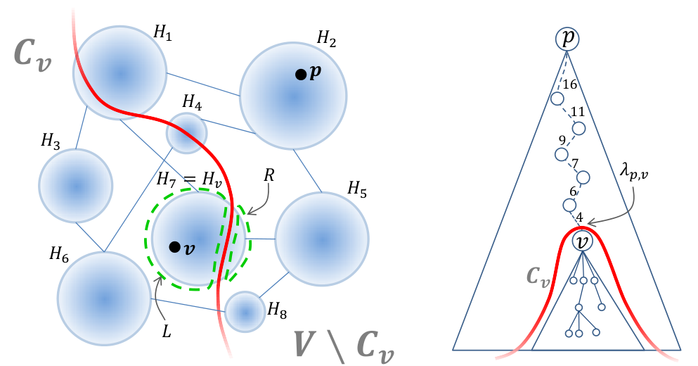
To handle Case 1 the algorithm simply asks a Max-Flow query between $p$ and each relevant node $u$ in each small expander $H$, i.e., $|H|<w/8$. Clearly, if $v$ happens to be in a small expander it gets queried and its optimal cut is found with probability $1$. The slightly trickier part is arguing that only $t=O(\sqrt{n})$ queries are performed: any queried node $u$ has degree $\geq w$ (since it is relevant) while a small expander only has $<w/8$ nodes, thus overall $\Omega(tw)$ edges are outside the expanders. But the expander decomposition guarantees that only $O(|E|/\sqrt{w})$ edges are outside the expanders, and thus $t=O(|E|/w^{1.5})$; in the hardest case where $w=\Omega(n)$ this is $t=O(\sqrt{n})$. The fact that the auxiliary graph $G_{i}$ is a multigraph does not matter, because the expander decomposition is for $G$. This is the only case in the algorithm that requires $G$ to be simple;¹⁰¹⁰ 10 Besides, of course, to speed up the Max-Flow queries: since all $\lambda_{s,t}\leq n$, the time bound of Karger and Levine [KL15] is $\tilde{O}(n^{2})$. the argument is similar to [KT19, Observation 5].

Handling Case 2 involves a surprising Isolating-Cuts procedure that can almost compute single-source all-sinks Max-Flow with $O(\log n)$ queries to Max-Flow. It is a tricky but lightweight reduction that only involves contracting subsets of nodes.

This procedure is quite strong in the sense that it solves hard cases with $\tilde{O}(1)$ Max-Flow queries when other approaches require $\Omega(n)$ queries, for instance in cases where all subtrees are small (see Section 3). But it is also weak in the sense that there is no way to distinguish the correct answers from fake ones. Nodes with large subtrees may never be isolated yet the procedure returns a (fake) small cut that, if used by the algorithm, could lead to a wrong tree. The canonical such example is discussed in Section 3 as it motivates the use of an expanders-based approach.

The Isolating-Cuts procedure is handy in Case 2 where the algorithm takes each expander $H$ with $|H|\geq w/8$ (there are only $O(n/w)=O(1)$ such expanders) and guesses that $H=H_{v}$ and that it is a large righty expander, i.e., $|L|\leq 2\sqrt{w}$. In this case, if indeed $v\in H$, it is possible to pick $t=\tilde{O}(\sqrt{w})$ sets of terminals $C_{1},\ldots,C_{t}$ such that at least one of them isolates $v$: for each $i^{\prime}\in[t]$ include each node $u\in H$ into $C_{i^{\prime}}$ with probability $1/\sqrt{w}$. For a set $C_{i^{\prime}}$ to isolate $v$, it must (1) pick $v$ and (2) not pick any other node from $L$, which happens with probability $\Omega(1/\sqrt{w})$; therefore, with high probability at least one of the sets $C_{1},\ldots,C_{t}$ isolates $v$. The Isolating-Cuts procedure is called for each $C_{i^{\prime}}$, getting new estimates for all $v\in V_{i}$; a total of $\tilde{O}(\sqrt{w})$ queries for all large expanders. The intuition is that a large righty expander helps the algorithm pick a good set of terminals that isolates $v$, a highly nontrivial task if $v$’s subtree is large, by focusing the attention on a component that (presumably) only contains few nodes from the subtree. Indeed, the Isolating-Cuts procedure is not as helpful in Case 3 where $H_{v}$ is a large lefty expander and $|L|$ can be up to $n$, since randomly chosen terminals from $H$ are unlikely to leave $v$ isolated.

To handle the final Case 3, the algorithm identifies the set $\text{Top}_{k}(H)$ of the top $k=3\sqrt{n}+1$ nodes in terms of their $c^{\prime}(u)$ estimate for each large expander $H$, and performs a Max-Flow query for each one. Since there are only $O(n/w)=O(1)$ large expanders, only $O(\sqrt{n})$ queries are performed. Suppose that $v$ is indeed in a large lefty expander $H_{v}$ with $|R|\leq 2\sqrt{w}$. The argument is that $v$ must be among the queried nodes unless there are $>\sqrt{n}$ undone nodes $u\in C_{v}$ in its subtree.¹²¹² 12 Recall that a node $u$ is undone if $c^{\prime}(u)>\lambda_{p,u}$ and done if $c^{\prime}(u)=\lambda_{p,u}$. This is because any done node $u\in C_{v}$ has $c^{\prime}(u)=\lambda_{p,u}\leq\lambda_{p,v}$, since $C_{v}$ is a valid $(p,u)$-cut of value $\lambda_{p,v}$, while $\lambda_{p,v}<c^{\prime}(v)$ (otherwise $v$ is already done). Therefore, any node $u\in H_{v}$ with $c^{\prime}(u)\geq c^{\prime}(v)$ can either be in $R\subseteq V\setminus C_{v}$ or it could be an undone node in $L\subseteq C_{v}$. There are at most $2\sqrt{w}+\sqrt{n}$ such nodes in total; thus $v\in\text{Top}_{k}(H_{v})$. Observe that this argument does not work in Case 2 where $H_{v}$ is a large righty expander and $|R|$ can be up to $n$, since the nodes in $R$ might have larger connectivity than $v$.

Finally, if $v$ happens to be in a large lefty expander when its subtree contains $>\sqrt{n}$ undone nodes, then the algorithm is not guaranteed to find $C_{v}$ in this iteration of procedure Expanders-Guided Querying. ($v$ is a red node with many red nodes in its subtree.) Soon enough, within $O(\log n)$ iterations, the algorithm gets to a point where most of $v$’s subtree has become done and then $C_{v}$ is found. (The green from the leaves quickly “infects” the entire tree.)

On the hardness side, the only related lower bounds are for All-Pairs Max-Flow in the harder settings of directed graphs [AWY18, KT18, AGI+19] or undirected graphs with node weights [AKT20b], where Gomory-Hu trees cannot even exist, because the $\Omega(n^{2})$ minimum cuts might all be different [HL07] (see therein also an interesting exposition of certain false claims made earlier). In particular, SETH gives an $n^{3-o(1)}$ lower bound for weighted sparse directed graphs [KT18] and the $4$-Clique conjecture gives an $n^{\omega+1-o(1)}$ lower bound for unweighted dense directed graphs [AGI+19]. Nontrivial algorithms are known for unweighted directed graphs, with time $O(m^{\omega})$ [CLL13] (fast matrix multiplication techniques have only been helpful in directed graphs so far), and also for special graph classes such as planar [LNSW12] and bounded-treewidth [ACZ98, AKT20a]. Moreover, algorithms exist for the case we only care about pairs of nodes whose Max-Flow value is bounded by small $k$ [BHKP07, GILP16, AGI+19]. Generalizations of the Gomory-Hu tree to other cut requirements such as multiway cuts or cuts between groups of nodes have also been studied [Has88, Has90, Has91, Har01, EH05, CKK16].

Coming up with faster constructions of a Gomory-Hu tree at the cost of approximations has also been of interest, see e.g. [Pan16], with only few successful approaches so far. One approach is to sparsify the graph into $m^{\prime}=\tilde{O}(\varepsilon^{-2}n)$ edges in randomized $\tilde{O}(m)$ time using the algorithm of Benczur and Karger [BK15] (or its generalizations), and then apply an exact Gomory-Hu tree algorithm on the sparse (but weighted) graph. Unfortunately, even when aiming for an approximate tree, each query throughout the Gomory-Hu (or the new) algorithm must be exact (see [Pan16, AKT20a]). Therefore, with current Max-Flow algorithms, a $(1+\varepsilon)$-approximate Gomory-Hu tree of unweighted graphs can be constructed in $\tilde{O}(\varepsilon^{-2}n^{2.5})$ time. Using a different approach that produces a flow-equivalent tree (rather than a cut-equivalent tree, meaning that the minimum cuts in the tree, viewed as node bipartitions, might not correspond to minimum cuts in the graph), one can design a $(1+\varepsilon)$-All-Pairs Max-Flow algorithm that runs in time $\tilde{O}(n^{2})$ [AKT20a]. Finally, one can use Räcke’s approach to compute a cut-sparsifier tree [Räc02], which has a stronger requirement (it approximates all cuts of $G$) but can only give polylogarithmic approximation factors. Its fastest version runs in almost-linear time $m^{1+o(1)}$ and achieves $O(\log^{4}n)$-approximation [RST14].

Cut-equivalent trees have appeared in countless application domains. One example is the pioneering work of Wu and Leahy [WL93] in 1993 on image segmentation using Gomory-Hu tree that has evolved into the graph cuts paradigm in computer vision. Another example is in telecommunications where Hu [Hu74] showed that the Gomory-Hu tree is the optimal solution to the minimum communication spanning tree problem; consequently there is interest in characterizing which graphs have a Gomory-Hu tree that is a subgraph [KV12, NS18]. In mathematical optimization, a seminal paper of Padberg and Rao [PR82] uses the Gomory-Hu tree to find odd cuts that are useful for the $b$-matching problem (and that have been used in a breakthrough NC algorithm for perfect matching in planar graphs [AV20]). The question of how the Gomory-Hu tree changes with the graph has arisen in applications such as energy and finance and has been investigated, e.g. [PQ80, BBDF06, HW13], starting with Elmaghraby in 1964 [Elm64] and up until very recently [BGK20]. Motivated by the need of a scalable algorithm for Gomory-Hu Tree, Akiba et al. [AIS+16] have recently introduced a few heuristic ideas for getting a subcubic complexity in social networks and web graphs. Earlier, Goldberg and Tsioutsiouliklis [GT01] conducted an experimental comparison of the Gomory-Hu and Gusfield’s algorithms.

A key ingredient of our Gomory-Hu tree algorithm is an expander-decomposition of the graph [KVV04, OV11, OSV12, ST13, SW19, CGL+20]. Such decompositions have led to several breakthroughs in algorithms for basic problems in the past decade, e.g. [ST14, KLOS14, NSW17]. A typical application solves the problem on each expander and then somehow combines the answers, treating each expander as a node. The clique-like nature of each expander and the sparsity of the outer graph lead to gains in efficiency. This approach does not seem helpful for Gomory-Hu tree since there may not be any connection between the tree and the decomposition. The application in this paper is more reminiscent of recent deterministic Global-Min-Cut algorithms [KT19, Sar21, LP20], but is also different from those (see Complication 5 in Section 1.3).

A partition tree $T$ of a graph $G=(V,E)$ is a tree whose nodes $1,\dots,l$ are super-nodes, which means that each node $i$ is associated with a subset $V_{i}\subseteq V$; and these super-nodes form a disjoint partition $V=V_{1}\sqcup\cdots\sqcup V_{l}$. An auxiliary graph $G_{i}$ is constructed from $G$ by merging nodes that lie in the same connected component of $T\setminus\{i\}$. For example, if the current tree is a path on super-nodes $1,\ldots,l$, then $G_{i}$ is obtained from $G$ by merging $V_{1}\cup\cdots\cup V_{i-1}$ into one contracted node and $V_{i+1}\cup\cdots\cup V_{l}$ into another contracted node. We will use the notations $n_{i}:=\lvert V_{i}\rvert$, $m_{i}:=\lvert E(G_{i})\rvert$, and $n^{\prime}_{i}:=\lvert V(G_{i})\rvert$. Note that $n_{i}^{\prime}\geq n_{i}$ since $V(G_{i})$ contains $V_{i}$ as well as some other contracted nodes, with $n_{i}^{\prime}=n_{i}$ only if the tree is a single node. The following is a brief description of the classical Gomory-Hu algorithm [GH61] (see Figure 3).

This algorithm constructs a cut-equivalent tree $\mathcal{T}$ in iterations. Initially, $\mathcal{T}$ is a single node associated with $V$ (the node set of $G$), and the execution maintains the invariant that $\mathcal{T}$ is a partition tree of $V$. At each iteration, the algorithm picks arbitrarily two graph nodes $s,t$ that lie in the same tree super-node $i$, i.e., $s,t\in V_{i}$. The algorithm then constructs from $G$ the auxiliary graph $G_{i}$ and invokes a Max-Flow algorithm to compute in this $G_{i}$ a minimum $(s,t)$-cut, denoted $C^{\prime}$. The submodularity of cuts ensures that this cut is also a minimum $(s,t)$-cut in the original graph $G$, and it clearly induces a disjoint partition $V_{i}=S\sqcup T$ with $s\in S$ and $t\in T$. The algorithm then modifies $\mathcal{T}$ by splitting super-node $i$ into two super-nodes, one associated with $S$ and one with $T$, that are connected by an edge whose weight is the value of the cut $C^{\prime}$, and further connecting each neighbor of $i$ in $\mathcal{T}$ to either $S$ or $T$ (viewed as super-nodes), depending on its side in the minimum $(s,t)$-cut $C^{\prime}$ (more precisely, neighbor $j$ is connected to the side containing $V_{j}$).

The algorithm performs these iterations until all super-nodes are singletons, which happens after $n-1$ iteration. Then, $\mathcal{T}$ is a weighted tree with effectively the same node set as $G$. It can be shown [GH61] that for every $s,t\in V$, the minimum $(s,t)$-cut in $\mathcal{T}$, viewed as a bipartition of $V$, is also a minimum $(s,t)$-cut in $G$, and of the same cut value. We stress that this property holds regardless of the choice made at each step of two nodes $s\neq t\in V_{i}$. A GH-Equivalent Partition Tree is a partition tree that can be obtained by a truncated execution of the Gomory-Hu algorithm, in the sense that there is a sequence of choices for the pairs $s\neq t\in V_{i}$ that can lead to such a tree. The following simple lemma describes the flexibility in designing cut-equivalent tree algorithms based on the Gomory-Hu framework.

Next, we discuss a few kinds of (GH-Equivalent) partition trees.

References

- [ABW15] Amir Abboud, Arturs Backurs, and Virginia Vassilevska Williams. Tight hardness results for LCS and other sequence similarity measures. In IEEE 56th Annual Symposium on Foundations of Computer Science, FOCS 2015, pages 59–78, 2015. doi:10.1109/FOCS.2015.14.
- [ACZ98] Srinivasa Rao Arikati, Shiva Chaudhuri, and Christos D. Zaroliagis. All-pairs min-cut in sparse networks. J. Algorithms, 29(1):82–110, 1998. doi:10.1006/jagm.1998.0961.
- [AGI+19] Amir Abboud, Loukas Georgiadis, Giuseppe F. Italiano, Robert Krauthgamer, Nikos Parotsidis, Ohad Trabelsi, Przemyslaw Uznanski, and Daniel Wolleb-Graf. Faster Algorithms for All-Pairs Bounded Min-Cuts. In 46th International Colloquium on Automata, Languages, and Programming (ICALP 2019), volume 132, pages 7:1–7:15, 2019. doi:10.4230/LIPIcs.ICALP.2019.7.
- [AIS+16] Takuya Akiba, Yoichi Iwata, Yosuke Sameshima, Naoto Mizuno, and Yosuke Yano. Cut tree construction from massive graphs. In 2016 IEEE 16th International Conference on Data Mining (ICDM), pages 775–780. IEEE, 2016.
- [AKT20a] Amir Abboud, Robert Krauthgamer, and Ohad Trabelsi. Cut-equivalent trees are optimal for min-cut queries. In 61st IEEE Annual Symposium on Foundations of Computer Science, FOCS 2020, pages 105–118, 2020. doi:10.1109/FOCS46700.2020.00019.
- [AKT20b] Amir Abboud, Robert Krauthgamer, and Ohad Trabelsi. New algorithms and lower bounds for all-pairs max-flow in undirected graphs. In Proceedings of the Thirty-First Annual ACM-SIAM Symposium on Discrete Algorithms, SODA ’20, page 48–61, USA, 2020. doi:10.1137/1.9781611975994.4.
- [AV20] Nima Anari and Vijay V Vazirani. Planar graph perfect matching is in nc. Journal of the ACM, 67(4):1–34, 2020.
- [AW14] Amir Abboud and Virginia Vassilevska Williams. Popular conjectures imply strong lower bounds for dynamic problems. In 55th IEEE Annual Symposium on Foundations of Computer Science, FOCS 2014, pages 434–443, 2014. doi:10.1109/FOCS.2014.53.
- [AW21] Josh Alman and Virginia Vassilevska Williams. A refined laser method and faster matrix multiplication. In Proceedings of the 2021 ACM-SIAM Symposium on Discrete Algorithms, SODA 2021, pages 522–539. SIAM, 2021. doi:10.1137/1.9781611976465.32.
- [AWY18] Amir Abboud, Virginia Vassilevska Williams, and Huacheng Yu. Matching triangles and basing hardness on an extremely popular conjecture. SIAM J. Comput., 47(3):1098–1122, 2018. doi:10.1137/15M1050987.
- [BBDF06] Dominique Barth, Pascal Berthomé, Madiagne Diallo, and Afonso Ferreira. Revisiting parametric multi-terminal problems: Maximum flows, minimum cuts and cut-tree computations. Discrete Optimization, 3(3):195–205, 2006.
- [BCH+08] Anand Bhalgat, Richard Cole, Ramesh Hariharan, Telikepalli Kavitha, and Debmalya Panigrahi. Efficient algorithms for Steiner edge connectivity computationand Gomory-Hu tree construction for unweighted graphs. Unpublished full version of [BHKP07], 2008. URL: http://hariharan-ramesh.com/papers/gohu.pdf.
- [BENW16] Glencora Borradaile, David Eppstein, Amir Nayyeri, and Christian Wulff-Nilsen. All-pairs minimum cuts in near-linear time for surface-embedded graphs. In 32nd International Symposium on Computational Geometry, volume 51 of SoCG ’16, pages 22:1–22:16. Schloss Dagstuhl–Leibniz-Zentrum fuer Informatik, 2016. doi:10.4230/LIPIcs.SoCG.2016.22.
- [BGK20] Surender Baswana, Shiv Gupta, and Till Knollmann. Mincut sensitivity data structures for the insertion of an edge. In 28th Annual European Symposium on Algorithms (ESA 2020). Schloss Dagstuhl-Leibniz-Zentrum für Informatik, 2020.
- [BHKP07] Anand Bhalgat, Ramesh Hariharan, Telikepalli Kavitha, and Debmalya Panigrahi. An Gomory-Hu tree construction algorithm for unweighted graphs. In 39th Annual ACM Symposium on Theory of Computing, STOC’07, pages 605–614. ACM, 2007. doi:10.1145/1250790.1250879.
- [BK15] Karl Bringmann and Marvin Kunnemann. Quadratic Conditional Lower Bounds for String Problems and Dynamic Time Warping. In Proc. of 56th FOCS, pages 79–97, 2015.
- [BSW15] Glencora Borradaile, Piotr Sankowski, and Christian Wulff-Nilsen. Min -cut oracle for planar graphs with near-linear preprocessing time. ACM Trans. Algorithms, 11(3), 2015. doi:10.1145/2684068.
- [BW09] Nikhil Bansal and Ryan Williams. Regularity lemmas and combinatorial algorithms. In 50th Annual IEEE Symposium on Foundations of Computer Science, FOCS 2009, pages 745–754, 2009. doi:10.1109/FOCS.2009.76.
- [CGI+16] Marco L. Carmosino, Jiawei Gao, Russell Impagliazzo, Ivan Mihajlin, Ramamohan Paturi, and Stefan Schneider. Nondeterministic extensions of the strong exponential time hypothesis and consequences for non-reducibility. In Proceedings of the 2016 ACM Conference on Innovations in Theoretical Computer Science, ITCS ’16, pages 261–270. ACM, 2016. doi:10.1145/2840728.2840746.
- [CGL+20] Julia Chuzhoy, Yu Gao, Jason Li, Danupon Nanongkai, Richard Peng, and Thatchaphol Saranurak. A deterministic algorithm for balanced cut with applications to dynamic connectivity, flows, and beyond. In 61st IEEE Annual Symposium on Foundations of Computer Science, FOCS 2020, pages 1158–1167. IEEE, 2020. doi:10.1109/FOCS46700.2020.00111.
- [CH03] Richard Cole and Ramesh Hariharan. A fast algorithm for computing steiner edge connectivity. In Proceedings of the 35th Annual ACM Symposium on Theory of Computing, STOC ’03, pages 167–176. ACM, 2003. doi:10.1145/780542.780568.
- [Cha12] Timothy M. Chan. All-pairs shortest paths for unweighted undirected graphs in o(mn) time. ACM Trans. Algorithms, 8(4):34:1–34:17, 2012. doi:10.1145/2344422.2344424.
- [Cha15] Timothy M. Chan. Speeding up the four Russians algorithm by about one more logarithmic factor. In Proceedings of the Twenty-Sixth Annual ACM-SIAM Symposium on Discrete Algorithms, SODA 2015, pages 212–217. SIAM, 2015. doi:10.1137/1.9781611973730.16.
- [CIP06] Chris Calabro, Russell Impagliazzo, and Ramamohan Paturi. A duality between clause width and clause density for SAT. In 21st Annual IEEE Conference on Computational Complexity, CCC 2006, pages 252–260, 2006. doi:10.1109/CCC.2006.6.
- [CKK16] Rajesh Chitnis, Lior Kamma, and Robert Krauthgamer. Tight bounds for gomory-hu-like cut counting. In 42nd International Workshop on Graph-Theoretic Concepts in Computer Science, volume 9941 of Lecture Notes in Computer Science, pages 133–144, 2016. doi:10.1007/978-3-662-53536-3\_12.
- [CLL13] Ho Yee Cheung, Lap Chi Lau, and Kai Man Leung. Graph connectivities, network coding, and expander graphs. SIAM Journal on Computing, 42(3):733–751, 2013. doi:10.1137/110844970.
- [CW87] Don Coppersmith and Shmuel Winograd. Matrix multiplication via arithmetic progressions. In Proceedings of the 19th Annual ACM Symposium on Theory of Computing, pages 1–6, 1987.
- [Edm70] Jack Edmonds. Submodular functions, matroids, and certain polyhedra. Combinatorial structures and their applications, pages 69–87, 1970.
- [EH05] Ori Einstein and Refael Hassin. The number of solutions sufficient for solving a family of problems. Mathematics of Operations Research, 30(4):880–896, 2005.
- [Elm64] Salah E Elmaghraby. Sensitivity analysis of multiterminal flow networks. Operations Research, 12(5):680–688, 1964.
- [Gab91] Harold N. Gabow. Applications of a poset representation to edge connectivity and graph rigidity. In 32nd Annual Symposium on Foundations of Computer Science, pages 812–821, 1991. doi:10.1109/SFCS.1991.185453.
- [Gab95] Harold N. Gabow. A matroid approach to finding edge connectivity and packing arborescences. Journal of Computer and System Sciences, 50(2):259–273, 1995.
- [GH61] Ralph E. Gomory and Te C. Hu. Multi-terminal network flows. Journal of the Society for Industrial and Applied Mathematics, 9:551–570, 1961. URL: http://www.jstor.org/stable/2098881.
- [GH86] Frieda Granot and Refael Hassin. Multi-terminal maximum flows in node-capacitated networks. Discrete Applied Mathematics, 13(2-3):157–163, 1986.
- [GILP16] L. Georgiadis, G. F. Italiano, L. Laura, and N. Parotsidis. 2-edge connectivity in directed graphs. ACM Transactions on Algorithms, 13(1):9:1–9:24, 2016. doi:10.1145/2968448.
- [GMW20] Pawel Gawrychowski, Shay Mozes, and Oren Weimann. Minimum cut in time. In Artur Czumaj, Anuj Dawar, and Emanuela Merelli, editors, 47th International Colloquium on Automata, Languages, and Programming, ICALP 2020, volume 168 of LIPIcs, pages 57:1–57:15. Schloss Dagstuhl - Leibniz-Zentrum für Informatik, 2020. doi:10.4230/LIPIcs.ICALP.2020.57.
- [GNT20] Mohsen Ghaffari, Krzysztof Nowicki, and Mikkel Thorup. Faster algorithms for edge connectivity via random 2-out contractions. In Proceedings of the Fourteenth Annual ACM-SIAM Symposium on Discrete Algorithms, pages 1260–1279. SIAM, 2020.
- [GR98] Andrew V. Goldberg and Satish Rao. Beyond the flow decomposition barrier. J. ACM, 45(5):783–797, 1998. doi:10.1145/290179.290181.
- [GT01] Andrew V. Goldberg and Kostas Tsioutsiouliklis. Cut tree algorithms: an experimental study. Journal of Algorithms, 38(1):51–83, 2001.
- [Gus90] Dan Gusfield. Very simple methods for all pairs network flow analysis. SIAM Journal on Computing, 19(1):143–155, 1990.
- [Har01] David Hartvigsen. Compact representations of cuts. SIAM Journal on Discrete Mathematics, 14(1):49–66, 2001.
- [Has88] Refael Hassin. Solution bases of multiterminal cut problems. Mathematics of Operations Research, 13(4):535–542, 1988. doi:10.1287/moor.13.4.535.
- [Has90] Rafael Hassin. An algorithm for computing maximum solution bases. Operations research letters, 9(5):315–318, 1990.
- [Has91] Refael Hassin. Multiterminal xcut problems. Annals of Operations Research, 33(3):215–225, 1991.
- [HKP07] Ramesh Hariharan, Telikepalli Kavitha, and Debmalya Panigrahi. Efficient algorithms for computing all low edge connectivities and related problems. In Proceedings of the 18th Annual ACM-SIAM Symposium on Discrete Algorithms, pages 127–136. SIAM, 2007. URL: http://dl.acm.org/citation.cfm?id=1283383.1283398.
- [HL07] Refael Hassin and Asaf Levin. Flow trees for vertex-capacitated networks. Discrete Appl. Math., 155(4):572–578, 2007. doi:10.1016/j.dam.2006.08.012.
- [HRW20] Monika Henzinger, Satish Rao, and Di Wang. Local flow partitioning for faster edge connectivity. SIAM Journal on Computing, 49(1):1–36, 2020. doi:10.1137/18M1180335.
- [Hu74] Te C. Hu. Optimum communication spanning trees. SIAM Journal on Computing, 3(3):188–195, 1974. doi:10.1137/0203015.
- [HW13] Tanja Hartmann and Dorothea Wagner. Dynamic Gomory-Hu tree construction–fast and simple. arXiv preprint arXiv:1310.0178, 2013.
- [IP01] Russell Impagliazzo and Ramamohan Paturi. On the complexity of k-SAT. Journal of Computer and System Sciences, 62(2):367–375, March 2001. doi:10.1006/jcss.2000.1727.
- [Kar00] David R. Karger. Minimum cuts in near-linear time. Journal of the ACM, 47(1):46–76, 2000.
- [KL15] David R. Karger and Matthew S. Levine. Fast augmenting paths by random sampling from residual graphs. SIAM J. Comput., 44(2):320–339, 2015. doi:10.1137/070705994.
- [KLOS14] Jonathan A Kelner, Yin Tat Lee, Lorenzo Orecchia, and Aaron Sidford. An almost-linear-time algorithm for approximate max flow in undirected graphs, and its multicommodity generalizations. In Proceedings of the 25th Annual ACM-SIAM Symposium on Discrete Algorithms, pages 217–226. SIAM, 2014.
- [KS96] David R. Karger and Clifford Stein. A new approach to the minimum cut problem. Journal of the ACM, 43(4):601–640, 1996. doi:10.1145/234533.234534.
- [KT18] Robert Krauthgamer and Ohad Trabelsi. Conditional lower bounds for all-pairs max-flow. ACM Trans. Algorithms, 14(4):42:1–42:15, 2018. doi:10.1145/3212510.
- [KT19] Ken-ichi Kawarabayashi and Mikkel Thorup. Deterministic edge connectivity in near-linear time. J. ACM, 66(1):4:1–4:50, 2019. doi:10.1145/3274663.
- [KV12] Bernhard Korte and Jens Vygen. Combinatorial optimization, volume 2. Springer, 2012.
- [KVV04] Ravi Kannan, Santosh Vempala, and Adrian Vetta. On clusterings: Good, bad and spectral. Journal of the ACM, 51(3):497–515, 2004. doi:10.1145/990308.990313.
- [LNSW12] Jakub Lacki, Yahav Nussbaum, Piotr Sankowski, and Christian Wulff-Nilsen. Single source - all sinks Max Flows in planar digraphs. In Proc. of the 53rd FOCS, pages 599–608, 2012.
- [LP20] Jason Li and Debmalya Panigrahi. Deterministic min-cut in poly-logarithmic max-flows. In 61st IEEE Annual Symposium on Foundations of Computer Science, FOCS 2020, pages 85–92, 2020. doi:10.1109/FOCS46700.2020.00017.
- [LS14] Yin Tat Lee and Aaron Sidford. Path finding methods for linear programming: Solving linear programs in iterations and faster algorithms for Maximum Flow. In 55th Annual Symposium on Foundations of Computer Science, FOCS ’14, pages 424–433. IEEE Computer Society, 2014. doi:10.1109/FOCS.2014.52.
- [LS19] Yang P. Liu and Aaron Sidford. Faster energy maximization for faster maximum flow. CoRR, 2019. URL: http://arxiv.org/abs/1910.14276.
- [LS20] Yang P. Liu and Aaron Sidford. Unit capacity maxflow in almost time. CoRR, abs/2003.08929, 2020. URL: https://arxiv.org/abs/2003.08929, arXiv:2003.08929.
- [Mąd16] Aleksander Mądry. Computing maximum flow with augmenting electrical flows. In Proceedings of the 57th IEEE Annual Symposium on Foundations of Computer Science, FOCS ’16, pages 593–602. IEEE Computer Society, 2016. doi:10.1109/FOCS.2016.70.
- [MN20] Sagnik Mukhopadhyay and Danupon Nanongkai. Weighted min-cut: sequential, cut-query, and streaming algorithms. In Proceedings of the 52nd Annual ACM SIGACT Symposium on Theory of Computing, pages 496–509, 2020.
- [NI92a] Hiroshi Nagamochi and Toshihide Ibaraki. Computing edge-connectivity in multigraphs and capacitated graphs. SIAM J. Discret. Math., 5(1):54–66, 1992. doi:10.1137/0405004.
- [NI92b] Hiroshi Nagamochi and Toshihide Ibaraki. Linear time algorithms for finding -edge connected and -node connected spanning subgraphs. Algorithmica, 7:583–596, 1992. doi:10.1007/BF01758778.
- [NS18] Guyslain Naves and F Bruce Shepherd. When do Gomory-Hu subtrees exist? CoRR, 2018. URL: http://arxiv.org/abs/1807.07331.
- [NSW17] Danupon Nanongkai, Thatchaphol Saranurak, and Christian Wulff-Nilsen. Dynamic minimum spanning forest with subpolynomial worst-case update time. In 2017 IEEE 58th Annual Symposium on Foundations of Computer Science (FOCS), pages 950–961. IEEE, 2017.
- [OSV12] Lorenzo Orecchia, Sushant Sachdeva, and Nisheeth K. Vishnoi. Approximating the exponential, the Lanczos method and an -time spectral algorithm for balanced separator. In Proceedings of the 44th Annual ACM Symposium on Theory of Computing, pages 1141–1160, 2012. doi:10.1145/2213977.2214080.
- [OV11] Lorenzo Orecchia and Nisheeth K Vishnoi. Towards an SDP-based approach to spectral methods: A nearly-linear-time algorithm for graph partitioning and decomposition. In Proceedings of the 22nd Annual ACM-SIAM Symposium on Discrete Algorithms, pages 532–545. SIAM, 2011.
- [Pan16] Debmalya Panigrahi. Gomory-Hu trees. In Ming-Yang Kao, editor, Encyclopedia of Algorithms, pages 858–861. Springer New York, 2016. doi:10.1007/978-1-4939-2864-4_168.
- [PQ80] Jean-Claude Picard and Maurice Queyranne. On the structure of all minimum cuts in a network and applications. In Combinatorial Optimization II, pages 8–16. Springer, 1980.
- [PR82] Manfred W Padberg and M Ram Rao. Odd minimum cut-sets and -matchings. Mathematics of Operations Research, 7(1):67–80, 1982.
- [Räc02] Harald Räcke. Minimizing congestion in general networks. In Proceedings of the 43rd Symposium on Foundations of Computer Science, FOCS ’02, page 43–52. IEEE Computer Society, 2002. doi:10.1109/SFCS.2002.1181881.
- [RST14] Harald Räcke, Chintan Shah, and Hanjo Täubig. Computing cut-based hierarchical decompositions in almost linear time. In Proceedings of the 25th Annual ACM-SIAM Symposium on Discrete Algorithms, SODA ’14, page 227–238. SIAM, 2014. doi:10.1137/1.9781611973402.17.
- [Sar21] Thatchaphol Saranurak. A simple deterministic algorithm for edge connectivity. In 4th Symposium on Simplicity in Algorithms, SOSA 2021, pages 80–85. SIAM, 2021. doi:10.1137/1.9781611976496.9.
- [Sei95] Raimund Seidel. On the all-pairs-shortest-path problem in unweighted undirected graphs. Journal of computer and system sciences, 51(3):400–403, 1995.
- [ST13] Daniel A Spielman and Shang-Hua Teng. A local clustering algorithm for massive graphs and its application to nearly linear time graph partitioning. SIAM Journal on computing, 42(1):1–26, 2013.
- [ST14] Daniel A Spielman and Shang-Hua Teng. Nearly linear time algorithms for preconditioning and solving symmetric, diagonally dominant linear systems. SIAM Journal on Matrix Analysis and Applications, 35(3):835–885, 2014.
- [SW19] Thatchaphol Saranurak and Di Wang. Expander decomposition and pruning: Faster, stronger, and simpler. In Proceedings of the 30th Annual ACM-SIAM Symposium on Discrete Algorithms, SODA 2019, pages 2616–2635, 2019. doi:10.1137/1.9781611975482.162.
- [vdBLL+21] Jan van den Brand, Yin Tat Lee, Yang P. Liu, Thatchaphol Saranurak, Aaron Sidford, Zhao Song, and Di Wang. Minimum cost flows, MDPs, and -regression in nearly linear time for dense instances. CoRR, 2021. URL: http://arxiv.org/abs/2101.05719.
- [WL93] Zhenyu Wu and Richard Leahy. An optimal graph theoretic approach to data clustering: Theory and its application to image segmentation. IEEE transactions on pattern analysis and machine intelligence, 15(11):1101–1113, 1993.
- [WW18] Virginia Vassilevska Williams and R. Ryan Williams. Subcubic equivalences between path, matrix, and triangle problems. J. ACM, 65(5):27:1–27:38, 2018. doi:10.1145/3186893.
- [Yu18] Huacheng Yu. An improved combinatorial algorithm for boolean matrix multiplication. Inf. Comput., 261:240–247, 2018. doi:10.1016/j.ic.2018.02.006.
Appendix A An Alternative Proof of the Isolating-Cuts Procedure
This section gives a complete proof of Lemma 3.4 by generalizing the arguments in Section 3.1. The Lemma essentially follows from the very recent work of Li and Panigrahy [LP20, Theorem II.2] for Global-Min-Cut. We provide another proof both for completeness and because it could be of interest as it exploits the structure of the Gomory-Hu tree instead of using the submodularity of cuts directly. Let be an upper bound on Max-Flow in graphs with nodes, edges, and where the flow size is bounded by .
Lemma 3.4 (restated).
Given an undirected graph on nodes and total edges, a pivot node , and a set of connected vertices , let where be the latest minimum -cut for each . There is a deterministic -time algorithm that returns disjoint sets such that for all : if then .
We call a node isolated if it satisfies this condition. We begin by describing the algorithm, then continue to its analysis.
Algorithm.
First, we prove this theorem with additional edges of very large capacities and for , and then we show that we actually do not need these edges.
- 1.
We define a recursive procedure which operates as follows.
- (a)
If , denote the node in by , find , and return .
- (b)
Otherwise, if , do the following.
- i.
Similar to Section 3.1, connect with edges of capacity to every node in , and denote by the resulting graph.
- ii.
Denote by an arbitrary set of nodes from , and by the remaining nodes of .
- iii.
Split into and , connecting the newly added edges between nodes in and in to , and the newly added edges between nodes in and in to . Namely, for each edge where we add the edge to and for each edge where we add the edge to .
- iv.
Add an edge of capacity between between and , and denote the new graph .
- v.
Next, find , where and (and thus also and , since otherwise the weight of the cut would be at least , while any cut with and has weight at most ).
- vi.
Continue recursively by calling and where is after removing all edges of high capacities , and contracting , and is similar but after contracting .
Correctness.
We begin by a description of the structure of every cut-equivalent tree of , and then of every cut-equivalent of (see Figure 7).
Claim A.1.
The following structural claims hold. For every cut-equivalent tree of and every isolated node , has an edge of capacity between and , such that removing from results in a partition of the nodes into the two subtrees and such that , where and .
Proof.
This is simply true because the added edge of capacity must participate in every minimum -cut in , and that removing the edges of capacity from results in . ∎
Claim A.2.
For every cut-equivalent tree of and every node , has an edge of capacity between and , with a minimum -cut attached to , and symmetrically for every node , has an edge of capacity between and , with a minimum -cut attached to . In addition, must have connected to with an edge of capacity at least .
This is true similarly to Claim A.1, and as is on the same side as in every minimum cut in that is not a minimum -cut. ∎
We will show the following claim for graphs along the execution.
Claim A.3.
For every isolated node , if then (i.e., the nodes of have not been contracted).
Given claim A.3, it is easy to see that eventually will be contained in a recursive call that has exactly one connected node , and there is a valid option for a -cut. As a result, this cut will be returned, as required.
Proof of Claim A.3.
This is proved by induction on the recursion depth. The base case is depth , namely the input graph right after the preprocessing step, that is , which contains for every connected node . Let be a graph along the execution. Assuming that for a isolated node , it belongs to , and we will show that is contained in . Consider the graph in the previous depth upon which its , was constructed. Since , it holds by the induction hypothesis that . By the Claim A.2, must stick together in either side of , and thus (this is true since in every minimum -cut in ), as required. ∎
Running time.
Note that after iterations, we returned a cut for every node in . Furthermore, for every depth in the recursion, the total number of nodes in all graphs is bounded by , and of the edges by , and the total size of all flows queried in this depth is bounded by , the latter is correct since the super-nodes in a single depth form a partition tree, and so by Claim in [AKT20b] the total sum of all edge weights in these auxiliary graphs is bounded by .
Finally, as we will show shortly, we will actually not use the edges with capacity , and so the total flow queried simply becomes .
Lifting the assumption on heavy edges.
Finally, we note that the added weights are not really necessary. The algorithm would be the same, except that we do not add edges of high capacity. Instead, just before computing we define a graph where we contract and into , and also and into , and then find . Recall that is . Since in every it holds that and , partitions in the same way as some (considering super-nodes as the nodes they contain). This is because if we contract nodes on each side of a min cut but not across, then the same cut remains.